A System for Acquisition, Processing and Visualization of Image Time Series from Multiple Camera Networks

Abstract

A system for multiple camera networks is proposed for continuous monitoring of ecosystems by processing image time series. The system is built around the Finnish Meteorological Image PROcessing Toolbox (FMIPROT), which includes data acquisition, processing and visualization from multiple camera networks. The toolbox has a user-friendly graphical user interface (GUI) for which only minimal computer knowledge and skills are required to use it. Images from camera networks are acquired and handled automatically according to the common communication protocols, e.g., File Transfer Protocol (FTP). Processing features include GUI based selection of the region of interest (ROI), automatic analysis chain, extraction of ROI based indices such as the green fraction index (GF), red fraction index (RF), blue fraction index (BF), green-red vegetation index (GRVI), and green excess (GEI) index, as well as a custom index defined by a user-provided mathematical formula. Analysis results are visualized on interactive plots both on the GUI and hypertext markup language (HTML) reports. The users can implement their own developed algorithms to extract information from digital image series for any purpose. The toolbox can also be run in non-GUI mode, which allows running series of analyses in servers unattended and scheduled. The system is demonstrated using an environmental camera network in Finland.

1. Introduction

Webcam photography is an established way of monitoring the conditions in the environment, for instance for recreation purposes (ski resorts, hiking trails). However, webcam photography also has growing usage for scientific purposes; it can be applied to continuously monitor ecosystems [1].

Studies show that various phenomena of vegetation phenology can be analyzed by digital imagery. Different vegetation indices can be extracted for different geographical regions from digital images. For different ecosystems and illumination conditions, the indices vary in their performance on characterizing phenology events [1,2,3,4,5,6,7,8,9,10,11,12,13]. Correlation of the vegetation indices with other phenological data from other sensors has been studied [1,3,5,6,7,11,14]. Usage of vegetation indices to study ecological indicators, e.g., the nutrition of wild animals, has also been investigated [4,9,15,16]. The timing of seasonal changes is also analyzed from digital images [1,10,13,17]. Another topic for which digital image processing can be used is hydrology. Detection of the amount of snow cover from digital images is studied for different environments, e.g., mountains, glaciers [18,19,20,21,22].

The establishment of webcam networks intended for scientific monitoring of ecosystems is growing larger. The European Phenology Camera Network (EUROPhen) is a collection of cameras used for phenology across Europe [1]. In a similar way, the PhenoCam Network has cameras from 133 sites across North America and Europe [23]. Time-lapse digital camera images of Australian biomes for different locations are archived and distributed by the Australian Phenocam Network [24]. As a part of “Climate Change Indicators and Vulnerability of Boreal Zone Applying Innovative Observation and Modeling Techniques (MONIMET)” project, the MONIMET camera network was established to provide time-series of field observation and consists of about 30 cameras over Finland [25]. The Phenological Eyes Network (PEN) is another phenological camera network in Asia [26]. Digital images and other phenological data from such camera networks have been used in various studies [1,5,10,18,26].

Besides the networks particularly intended for scientific use, other types of camera networks such as traffic webcams, etc. can also be used for scientific purposes. Usage of traffic webcams for phenological studies was investigated by Morris et al. [27]. Camera networks for ski tracks and avalanche monitoring over mountains can also be used in the same manner. These networks provide potential data for hydrological purposes, e.g., analysis of snow cover [18,22]. On a larger scale, the status of webcams over the globe has also been studied. Freely available images from the global network of thousands of outdoor webcams have great potential to be used for scientific measurements. On the other hand, the task of obtaining and organizing these images is significantly challenging [28].

Numerous freely available software packages and tools have been developed to be used in analyzing images, but few focus on phenological monitoring [21,22,29,30]. The Phenopix R package is one example of a package with advanced features for image-based vegetation phenology [29]. It is designed to compute vegetation indices from digital images. The computations can be done either based on ROI averages or pixel values. For ROI-averaged analyses, the user is able to define ROIs using the GUI dedicated to that option. The package implements several data filtering and post processing methods. These include different curve fitting methods, different data filtering methods, extraction of phenophases and uncertainty analysis. The package also offers functions to visualize and save results. Other software packages also have features similar to Phenopix and others are different [21,22,30]. On the other hand, existing software lacks the features required to examine and benefit fully from existing and future camera networks. For achieving such goals, it is very important to establish systems, platforms and easy-to-use toolboxes for acquiring and handling images from different networks having different protocols and standards. Considering current and possible features, not only for analyzing images of comprehensive camera networks, but also for creating operational data extraction and processing with an easy to use toolbox, a more customized approach would be of high value. This approach is followed in FMIPROT. It is designed to be used as a basis for an automated processing system. This system is able to acquire and process images from multiple camera networks and visualize the processing results. It allows for storing all the configurations and the options used for analyses, so that the system can be used to create and maintain operational monitoring services. The plugin system allows the user to add new processing algorithms to FMIPROT, which makes it possible to benefit from advanced filtering, processing and post-processing methods in existing software packages.

The system architecture and its elements are described in Section 2. In Section 3, multiple examples of applications which can be used in phenology studies are presented. In Section 4, the system is demonstrated as an example for potential operational monitoring using the MONIMET camera network. In Section 5, the current system and the planned activities are discussed.

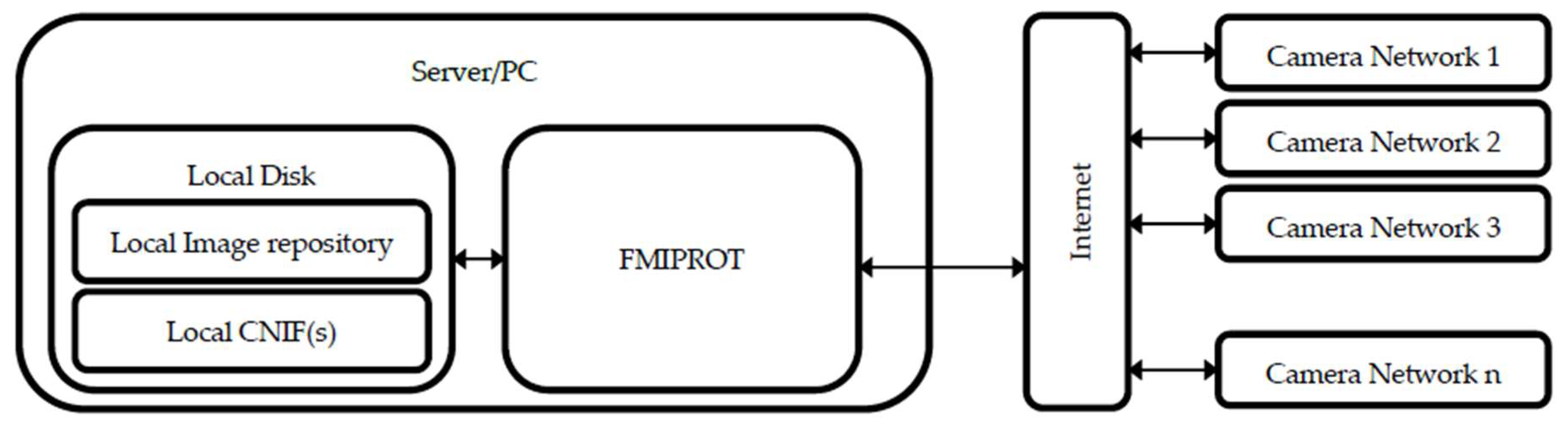
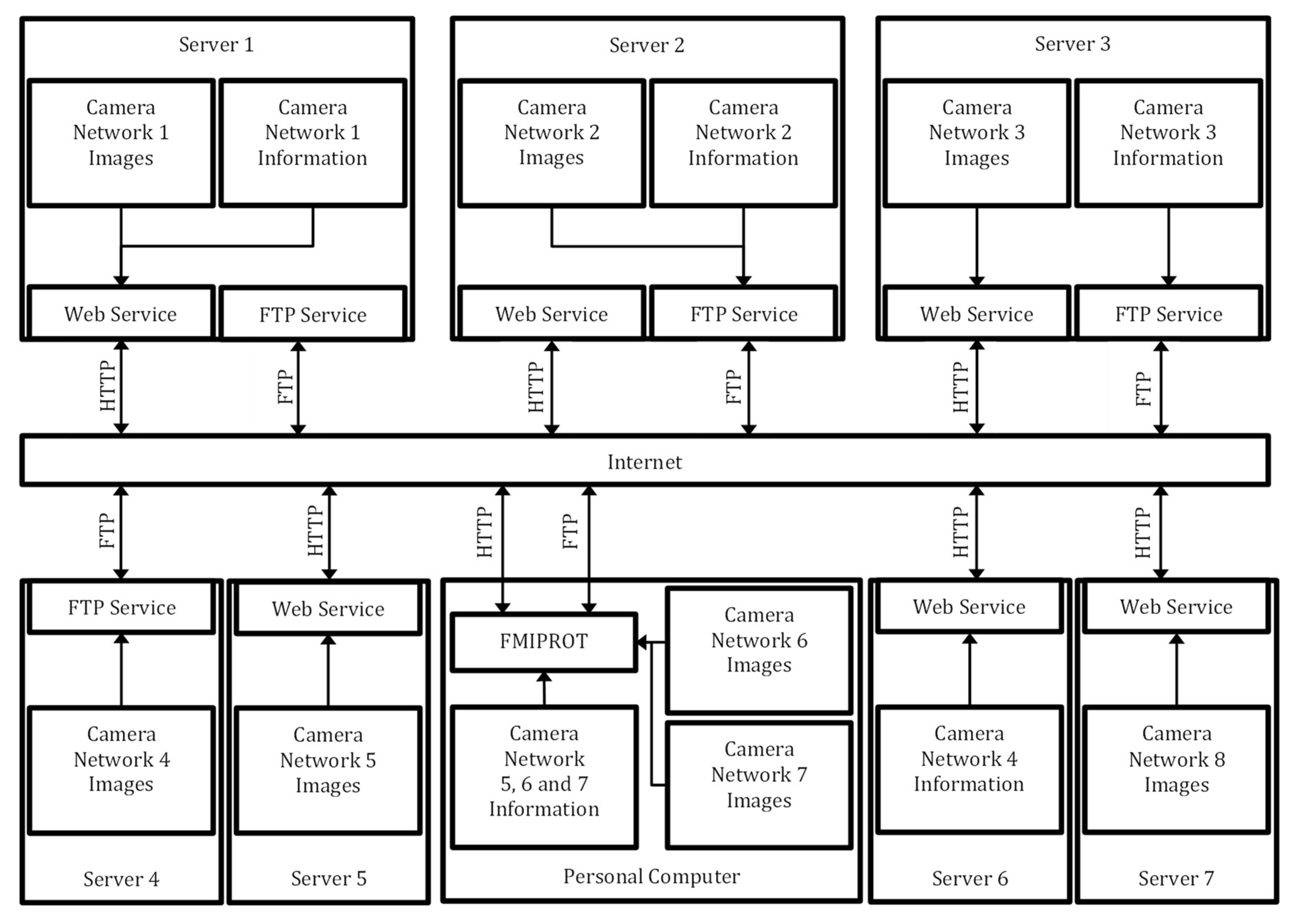
2. System Architecture

The image processing system presented in this paper consists of the Finnish Meteorological Image PROcessing Toolbox (FMIPROT), camera network information files (CNIF), local image repository and camera networks which include cameras, image repositories and online CNIFs. CNIFs are the files which store information on how to communicate with the camera networks. The whole system architecture is illustrated in Figure 1 and they are described in detail in the following sections.

The FMIPROT runs the entire system. The workflow, including all the features that are available with the GUI is explained in the toolbox subsection. Those features are used for standalone analyses and defining parameters for analyses to be used in operational monitoring. When running an operational system, the toolbox goes through a series of tasks for each scheduled run. These tasks can be divided into three phases: (1) acquisition; (2) processing; and (3) visualization. It starts from the acquisition phase by using CNIFs and the temporal selection information to list the images from repositories and download them if necessary. In the processing phase, if any older results exist for the same analysis, the timestamps from the results are read and listed. Using the list from the older results, and the file and timestamp lists from the acquisition phase, the images that are not processed, are read and processed according to the processing parameters. The old results that no longer fit the temporal selection are removed and the new results are stored as raw data in files. In the visualization phase, an HTML report which includes temporal selection, processing parameters, hyperlinks to the raw data and interactive plots that visualize the results. This working flow of the proposed operational system with all tasks in the three phases is illustrated in Figure 2.

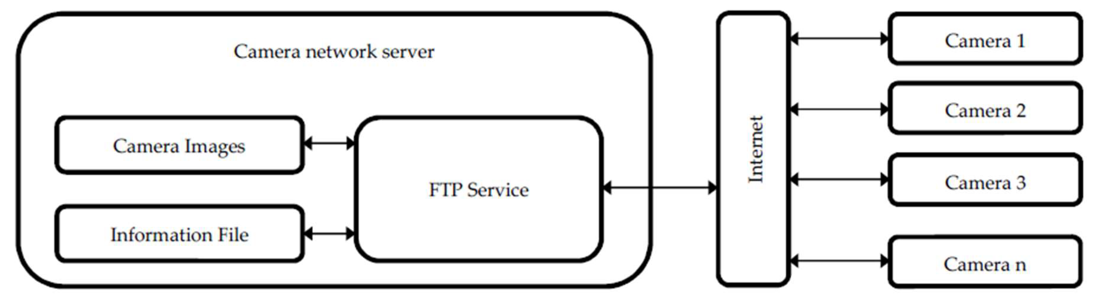
2.1. Camera Networks

A camera network can consist of one or multiple cameras. It is assumed to provide time series of images and an infrastructure for reception and storage of these images. A camera network information file (CNIF) is defined for each camera network used in FMIPROT. The CNIF includes the required information to communicate with the camera network, e.g., communication protocol, address, filename format. The CNIF can be created automatically using the GUI or manually by using technical information in the user manual. The CNIF can be stored on a local disk or in a remote server accessible by FTP or HTTP. This feature allows an operator of the camera network to maintain online CNIF(s) so that users can connect to the camera network and process the images using FMIPROT.

FMIPROT can be utilized with various supported protocols and configurations for multiple camera networks. There is no restriction to use certain communication protocols together. In Figure 3, an example of using FTP for both CNIF and various cameras is illustrated. Another example is given in Figure 4, using FTP for various cameras and HTTP over a web service for the camera network information file. The MONIMET Camera Network, which consists of 28 cameras (26 operating) producing 30 image series from 14 different locations in Finland works with the same configuration given in Figure 4 [25].

FMIPROT can also be connected to multiple camera networks. Images from each configured camera network can be used with FMIPROT. Archived images from local disk can also be used. In this case, these archives should be defined as a separate camera network. In Figure 5, an example of using eight different camera networks with different configurations is illustrated with communication protocols.

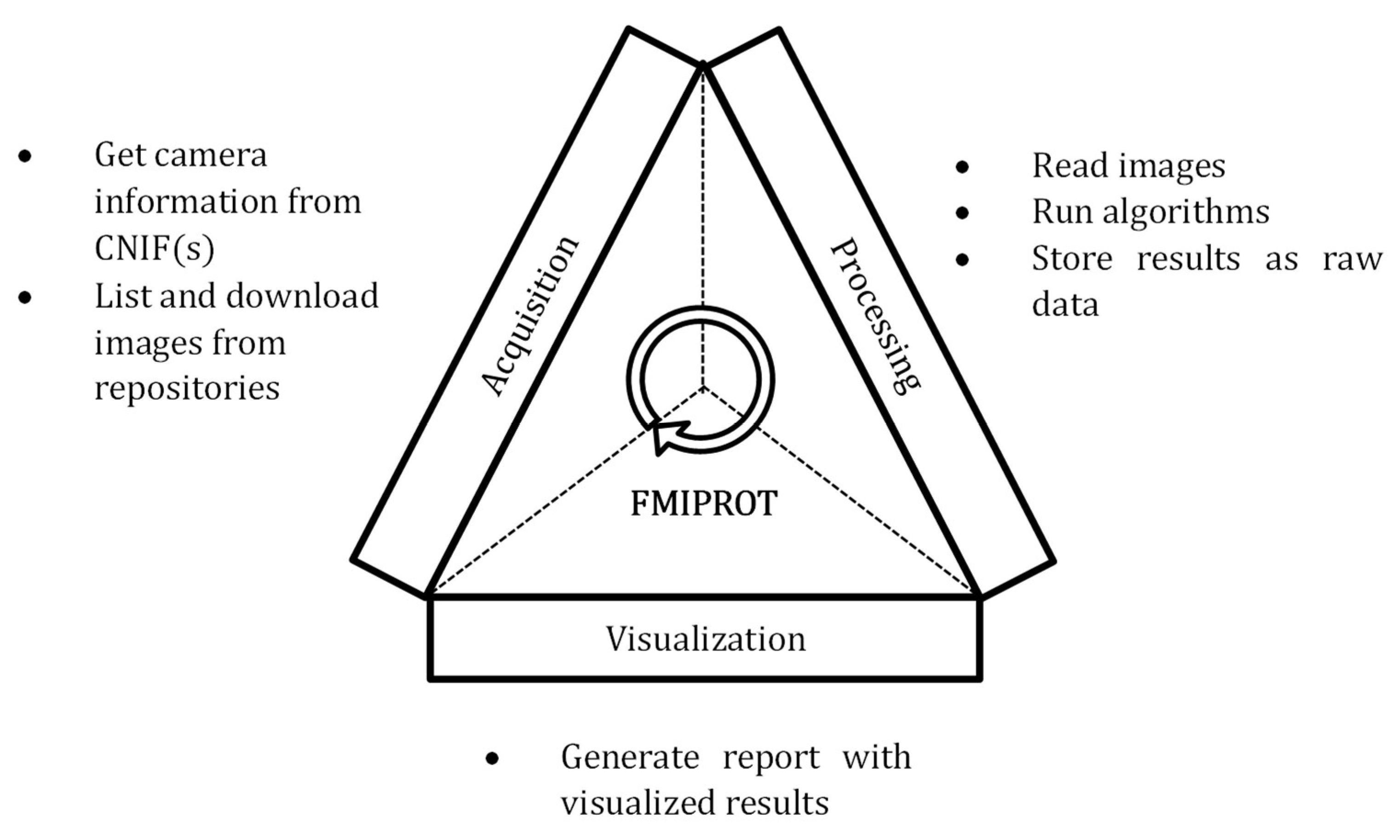
2.2. FMIPROT

2.2.1. Features

The main features of the FMIPROT are summarized below. All the detailed information about FMIPROT and the instructions can be found in the user manual [31].

The toolbox has a straightforward installation, which requires minimal computer skills. It does not have any software dependencies that require any extra installations (except old Linux systems). The interface is compact and user-friendly. All the actions required to create and run analyses can be performed using the GUI. It also has interactive interfaces where necessary, for example, to select ROIs. In Figure 6, an example for ROI selection (a) and an example for plotting of results (b) are shown. The analyses that are set up using GUI can also be run through the command line interface (CLI). It is possible to use the system for operational monitoring by using such features on remote servers.

FMIPROT provides automatic downloading and handling of images from multiple camera networks which can be added to the toolbox using the GUI. Users select the source(s) of images, i.e., the camera(s), and the software downloads the images from the camera network servers. The downloaded images are stored in a local directory used in the analyses before being cast to the processing functions. It is also possible to use proxy parameters to download the images from camera networks. For example, if the image repository of a camera is hosted on an FTP server, but the repository is also accessible as a directory on local disk, a “camera network proxy” can be used to read images from the disk directly instead of connecting to the FTP server. Similarly, different credentials for the FTP connection can be used. A user can store a setup file which includes only the username for the FTP connection to the image repository, which is only accessible by another user with the correct username and password. In that case, the toolbox will use the proxy to replace the credentials for the connection.

FMIPROT is designed so that the user can work with multiple analyses at the same time. The options and parameters for these multiple analyses are set up in a hierarchical way. For each run of the software, the user has a “Setup” which may have multiple “Scenarios”. These scenarios may also have multiple “Analyses”. This hierarchy allows the user to manage and run all analyses needed for a possible study or an operational product. An analysis is an algorithm which is applied to selected images. For example, calculating the “Greenness Index” with a specific algorithm is an analysis. A scenario is a combination of options that are set for one or multiple analyses to be done for images from a single camera. A setup is a collection of scenarios. Setups can be saved as an “FMIPROT Setup File”. Setup files can be loaded to the software for restoring all options. This feature makes it possible to share options for analyses in a more agile way.

Scenarios include options such as camera selection, temporal selection of images, threshold selections for filtering pixels and images, masking parameters for selecting ROIs and processing parameters for analyses.

At the end of running analyses, the toolbox creates a “setup report” which includes all the analysis options for each scenario and the results for each analysis on interactive plots. The report is in HTML format and uses JavaScript, thus it can be opened by any modern browser. In the report, there are also links to the data files of the results. When the report is automatically opened in the default browser after the analyses, users can reach the data files by these links. “Setup reports” can also be created without any results by using the option from the “setup” menu. The results can also be previewed in the GUI. The plots in the GUI can also be customized in numerous ways such as varying colors, lines and markers. There is also an option to save plots as image files.

FMIPROT has a plugin system, which allows users to add their own algorithms to the toolbox. It is planned to gradually implement a large variety of digital image processing algorithms to the FMIPROT. This feature allows users to plug in their own algorithms using advanced filtering, processing and post-processing methods in existing software packages while getting the benefits of the other existing features of the FMIPROT.

The software is able to check the temporal status of the image series of camera networks in a quantitative way. When the analysis is run, it scans all the images in the image repository and creates result files which include information about the number of images a time series. The result files can also be plotted to visualize the temporal coverage.

2.2.2. Software

FMIPROT is developed in Python programming language, using numerous freely available modules. The Python language is chosen for the ease of debugging and simplicity. It offers the possibility to run the code without compiling manually. The Python code is written in a modular way to increase readability and compatibility for possible updates and integrating codes written in other languages. The “Mahotas” package is used for image processing [32]. Tkinter is used for the graphical user interface.

The toolbox is available for both Linux and Windows platforms. The software packages can be downloaded from the FMIPROT website, at http://fmiprot.fmi.fi. They also include a detailed user manual with explanations on installation, usage and current algorithms used in the toolbox.

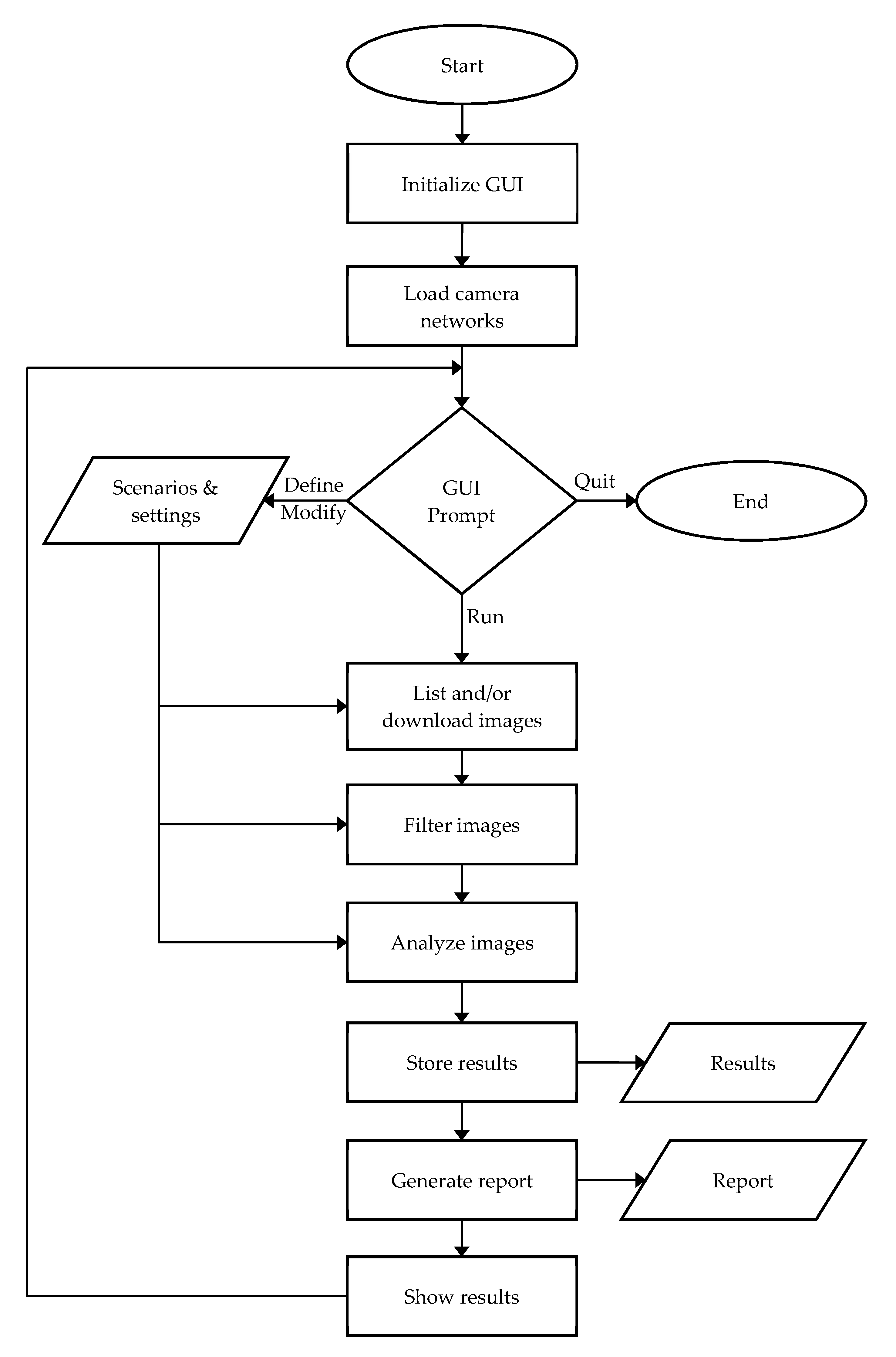
2.2.3. Workflow

On the code level, workflow of the program has many steps with complex relations due to the graphical user interface. For the sake of the processing system, the workflow is explained in a straightforward way by disregarding code level details.

When the software is started in GUI mode, it first initializes the user interface and reads the communication parameters of all camera networks. When it is ready, the user interface waits for the inputs to be processed. According to the inputs to the GUI, the software gives responses. After each response, the user interface waits for another input. Scenario options and settings are modified according to those inputs and changes are applied immediately. If requested, scenario options are stored on files. When the “Run” input is given, it starts the processing chain for the analysis of the images. During the processing, the interface does not respond to the inputs. It completes the necessary steps one by one, according to the scenario options and program settings. Those steps can be seen in Figure 7. After the processing chain, the interface opens both the “Result Viewer” menu and the “Setup report” to visualize the results. Finally, the user interface becomes responsive again for further interaction. If the program is run in non-GUI mode, the program skips the GUI prompt and directly runs the given command.

2.3. Image Processing Algorithms

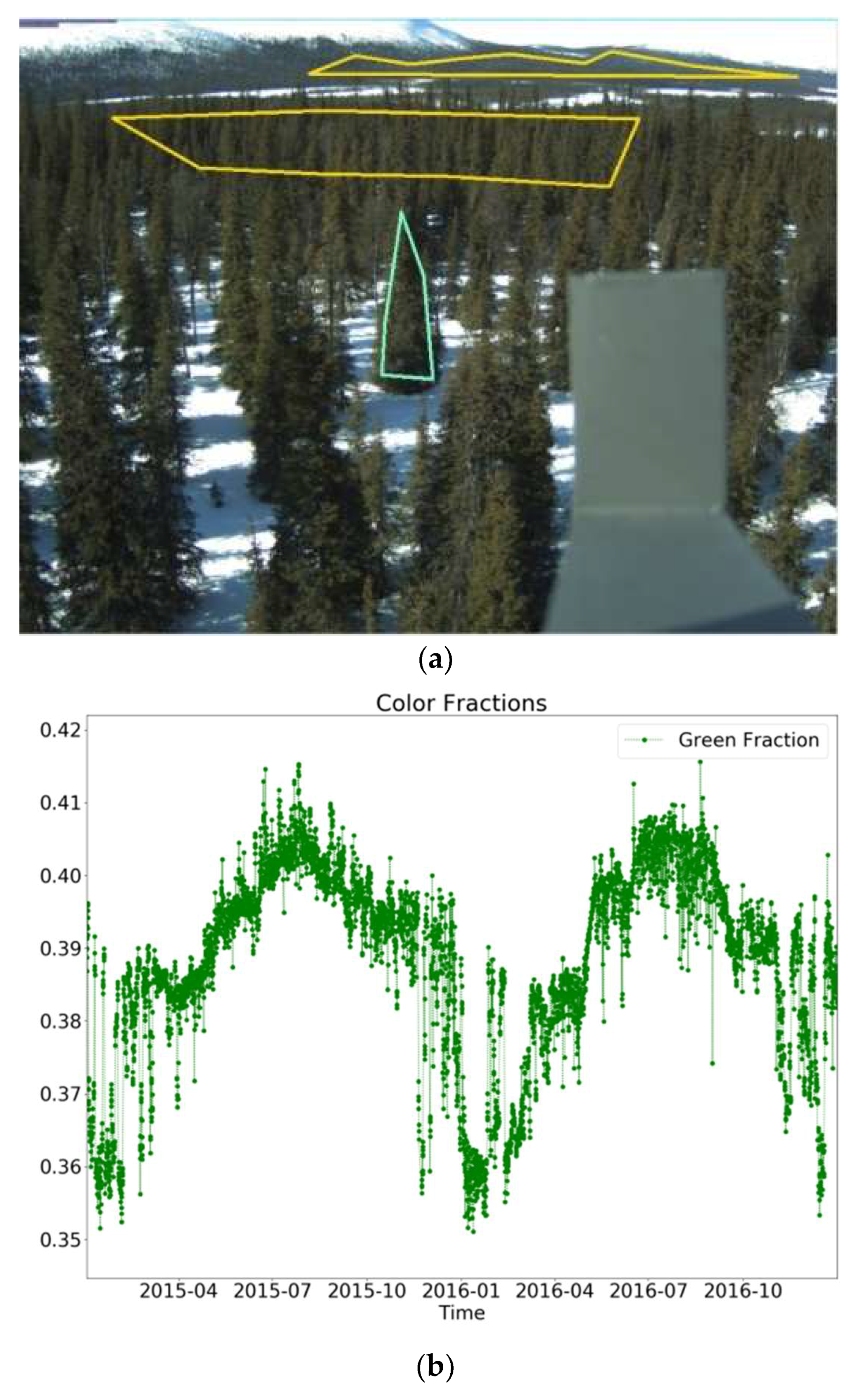
2.3.1. Color Fraction Indices (Color Chromatic Coordinates)

The color fraction index is the ratio of the sum (or mean) of the digital values of that color in a selected area to the sum (or mean) of digital values of all the color channels in that area in an image. The red fraction index (RF) (or alternatively red chromatic coordinate (RCC), strength of signal in red channel (S_R), red ratio, red index (RI), relative brightness of red channel), green fraction index (GF) (or alternatively green chromatic coordinate (GCC), strength of signal in green channel (S_G), green ratio, green index (GI), relative brightness of green channel), blue fraction index (BF) (or alternatively blue chromatic coordinate (BCC), strength of signal in blue channel (S_B), blue ratio, blue index (BI), relative brightness of blue channel), brightness (BR) and luminance (L) are calculated as;

RF = R/(R + G + B)

(1)

GF = G/(R + G + B)

(2)

BF = B/(R + G + B)

(3)

BR = R + G + B

(4)

L = 0.2989 R + 0.5870 G + 0.1140 B

(5)

where R, G and B are the digital numbers for the red, green and blue channel [7,11,13,14]. Brightness and luminance values are normalized to values between 0 and 1 in the analysis.

Time series of color fraction indices from webcam images can be used in the determination of phenological events. Changes in vegetation during seasons can be monitored using GF and RF, by detecting the dates that these changes occur [11,13]. The dates can be detected in post-processing by fitting GF and RF data which is produced by FMIPROT to sigmoid curves and finding the time of the fastest change by using second order derivatives of the fitted curves. It is planned to implement the extraction of phenophases by developing a plugin to use curve fitting methods from the Phenopix R package.

2.3.2. Green-Red Vegetation Index (GRVI)

The GRVI uses the difference between green and red colors. Because of the negative red term, GRVI can get negative or positive values depending on the season and target. During the growing season GRVI should result in positive values and during the dormant season it should result in negative values for deciduous species. The GRVI of an image is calculated as,

GRVI = (G − R)/(G + R)

(6)

where R and G are digital number values for red and green channels [6,7,8].

In terms of calculation of the index, GRVI is similar to the widely used NDVI, where near-infrared reflectance is used instead of green reflectance. The differences between these two indices are discussed by Motohka et al., where the applicability of GRVI for vegetation phenology is studied. One benefit of using GRVI is that it is better suited to detecting a subtle disturbance in the middle of the growing period [8]. Another advantage is that GRVI results in different patterns for seasonal change for deciduous forests and grassland.

2.3.3. Green Excess Index (2G-rbi)

The green excess index uses the difference between both green-red and green-blue. The GEI of an image is calculated as,

GEI = 2G − (R + B)

(7)

where R, G and B are digital number values for red, green and blue channels [11]. The mean GEI for ROIs is calculated by including pixels for which none of the channel digital values are zero.

2.3.4. Custom Color Index

This algorithm calculates an index from a mathematical formula entered by the user using average values of red, green and blue channels in ROIs. The formula supports sums, differences, multiplication, and division and operation priority by using parentheses. Using this algorithm, the user can analyze images using new indices or the indices which are in the literature but not implemented in the toolbox.

3. Examples of Applications

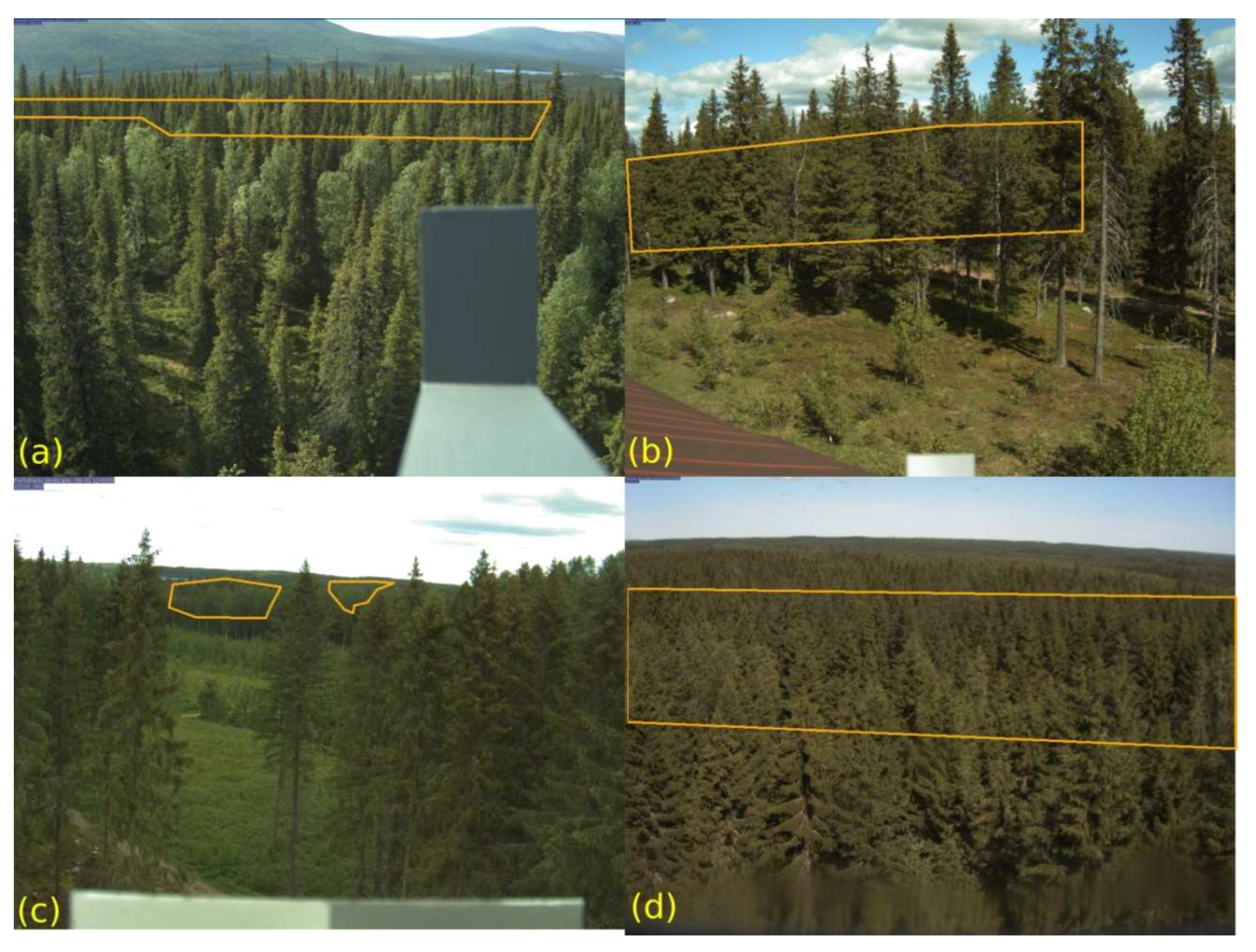
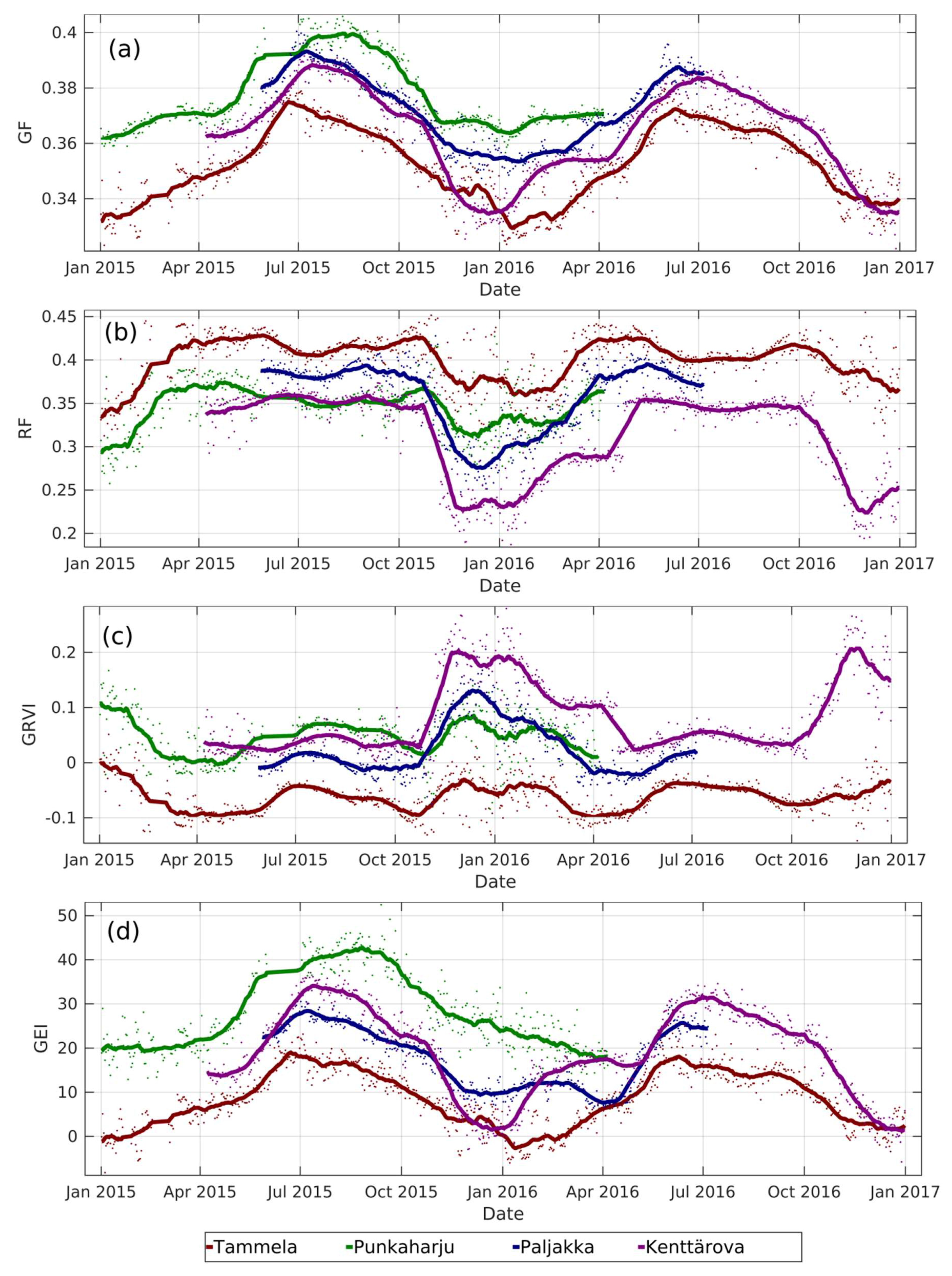
3.1. Extraction of Vegetation Indices for Same Species in Different Locations

Spruce stand is the dominant species in four sites of the MONIMET camera network. These sites are located on different latitudes and have different ecological conditions. In this example, canopy and landscape cameras from these sites are used to extract different vegetation indices for the canopy. Detailed information about the test sites can be found in Peltoniemi et al. [25]. The field of view for the selected cameras and ROIs chosen for the analyses are seen in Figure 8. Groups of trees close to each other are selected instead of individual trees and trees close to the camera are avoided. This selection is made in order to extract information about the overall canopy in the area and also decrease the effect of features and shadings between the trees. Date and times of day limits are set to select images taken between 10:15–13:45 in 2015 and 2016. This selection corresponds to about 7 images per day with 30 min intervals. No other filtering is set for selecting images. Vegetation indices are extracted from the images. GF, RF, GRVI and GEI for the image time series with smoothed lines are shown in Figure 9. The data points in the Figure are the values calculated by FMIPROT. The smoothed lines are produced for better visibility of the indices by using moving average filter on data points in 3-day windows, in a third party application.

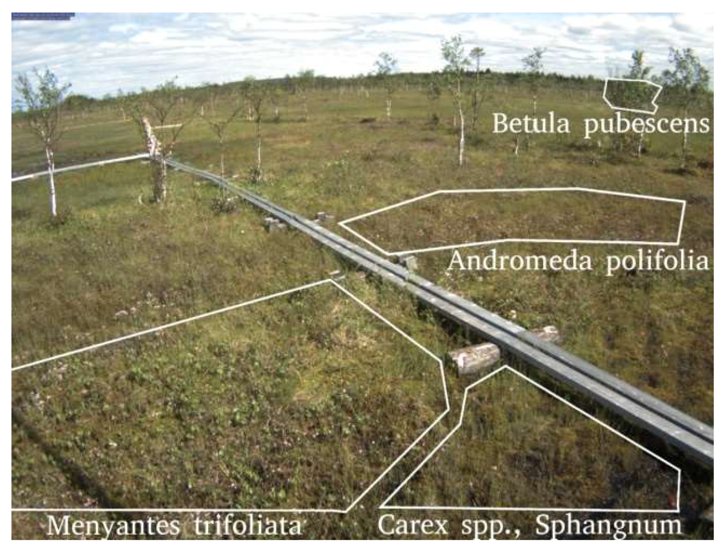
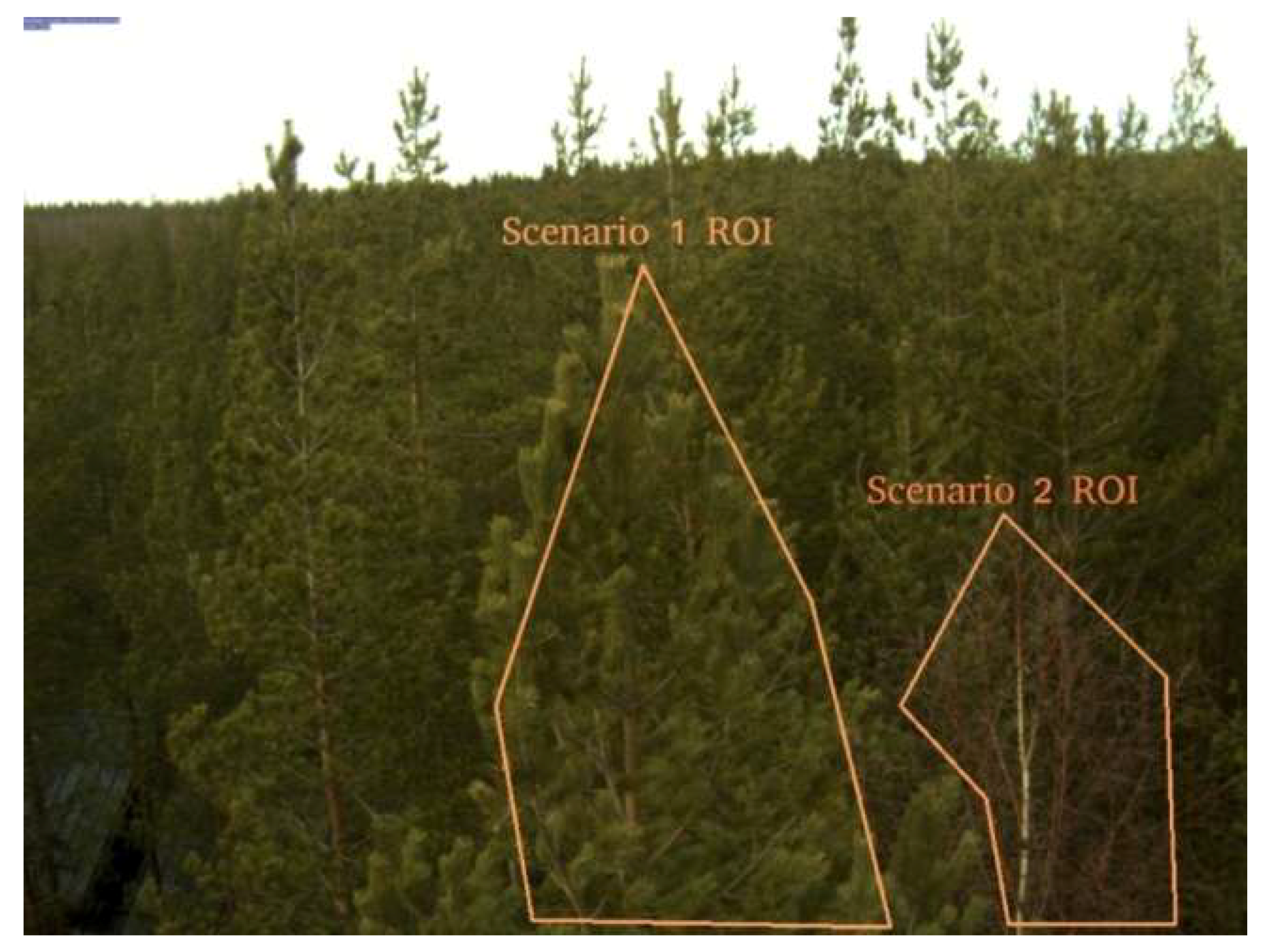
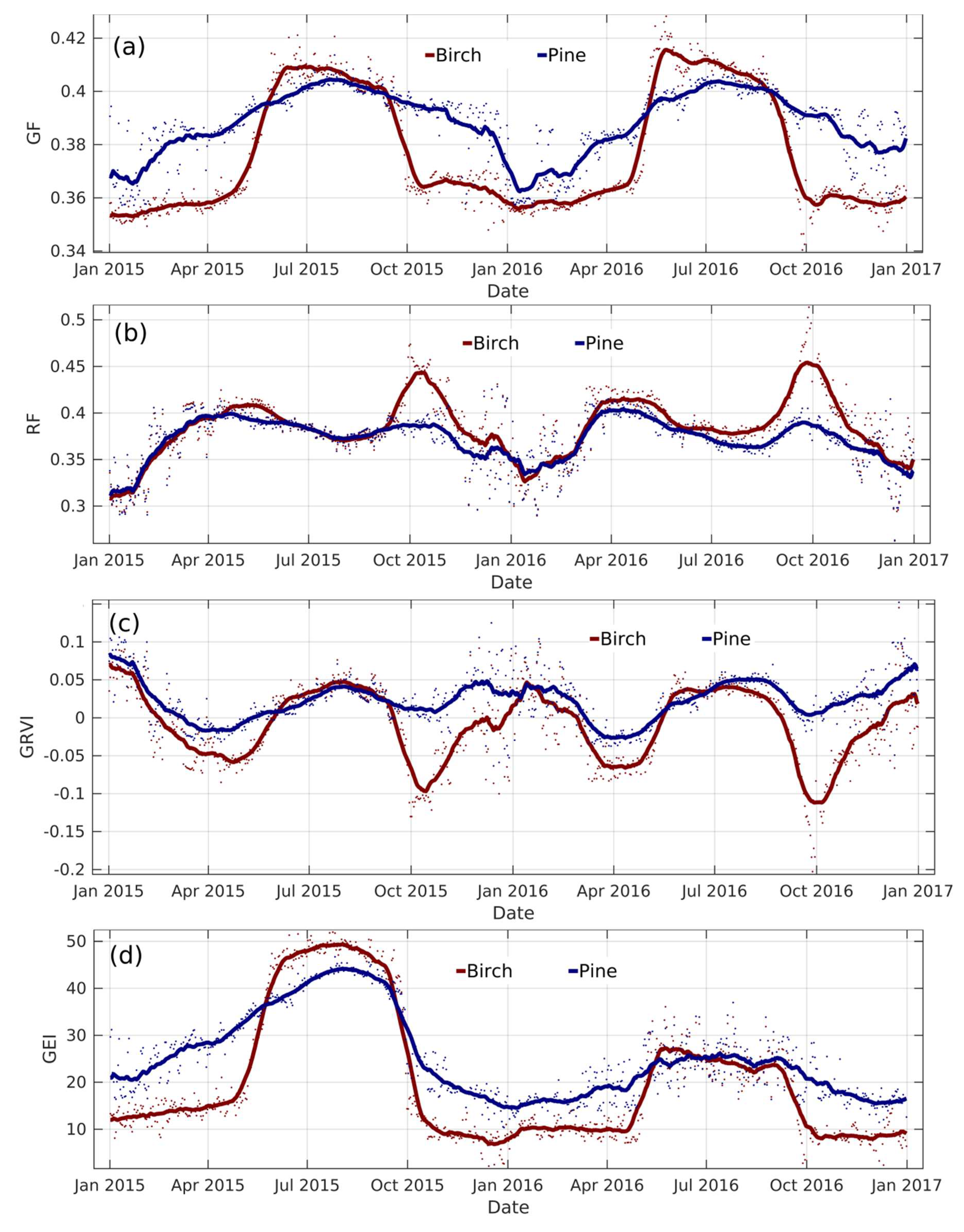
3.2. Extraction of Vegetation Indices for Two Species in a Single Camera Field of View

As an example, green and red fraction indices for two species seen from the Hyytiälä Crown Camera are calculated. ROIs are defined with polygons in Figure 10. Two scenarios are set in the toolbox with identical options except for the masks. “Scenario 1” has the polygon as the ROI on the right and “Scenario 2” has the polygon as the ROI on the left. The species for “Scenario 1” is Scots pine (Pinus sylvestris) and for “Scenario 2” is silver birch (Betula pendula). Date and times of day limits are set to select images taken between 10:15–13:45 in 2015 and 2016. This selection corresponds to about 7 images per day with 30 min intervals. No other filtering is set for selecting images. With these options, the software found and analyzed a total of 5018 images, taken between 1 January 2015 and 31 December 2016. Vegetation indices were extracted from the images. GF, RF, GRVI and GEI for the image time series with smoothed lines are shown in Figure 11. The data points in the Figure are the values calculated by FMIPROT. The smoothed lines are produced for better visibility of the indices by using a moving average filter on data points in 3-day windows, in a third party application.

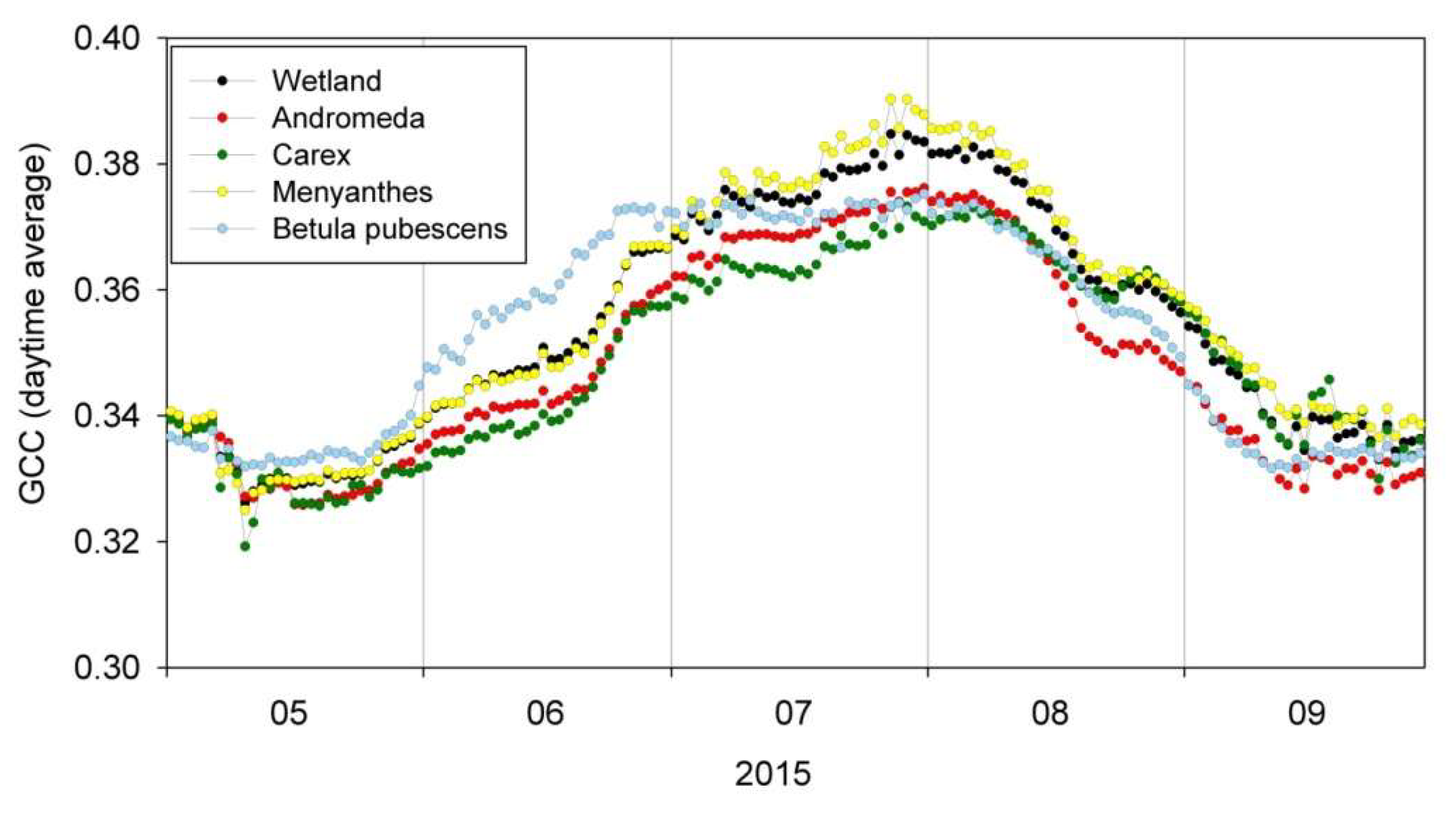
3.3. GCC Changes by Vegetation Patch in Sodankylä Wetland

In an ecosystem with heterogeneous vegetation patterns, typical for example, in wetlands, it is possible to track the GCC changes for several plant functional types. Linkosalmi et al. calculated GCC separately for four different target areas at their wetland site in Sodankylä [5]. The vegetation types on these target areas were dominated by (1) bog-rosemary (Andromeda polifolia) and other shrubs; (2) sedges (Carex spp.) and Sphagnum mosses; (3) big-leafed bogbean (Menyanthes trifoliate) and (4) downy birch (Betula pubescens) (Figure 12). For comparison, the GCC values were also analyzed for a larger area including the three first vegetation types.

The GCC values of the ROIs defined according to vegetation types show marked differences in the seasonal cycle, both in the timing of the major changes in spring and fall and in the magnitude of the maximum GCC (Figure 13). For example, downy birch had the fastest growth onset, while the big-leafed bogbean had the largest growing-season maximum.

4. Demonstration for Proposed Operational Monitoring

The system is demonstrated on a virtual machine. Operational targets are set up to monitor noon-time GF values for at least one ROI for multiple cameras in the MONIMET camera network. The results of monitoring should (a) always include the latest image with a maximum latency of 30 min; (b) be hosted on a web server so that it can be framed in the webpages for each camera in the MONIMET website [33].

The MONIMET camera network is part of MONIMET EU Life+ project (LIFE12 ENV/FI/000409) to establish knowledge in monitoring seasonal development of different types of ecosystems using low cost cameras [33]. In this demonstration, we used the images from the entire network, which consists of 15 sites and 28 cameras over Finland. Most cameras in the network are Stardot NetCam 5MP, which are designed for typical outdoor surveillance. The cameras have charge coupled device (CCD) sensors and produce optical images. The software of some of the cameras has been modified to produce also near-infrared images, which are not tested yet. The cameras transfer images over the internet to the image repositories using FTP every 30 or 60 min, depending on the camera. For the physical connection, Ethernet cables are used in sites where it is available through the infrastructure and by cellular modems where cable connection is not available. Twenty-seven of the cameras from 14 sites in the network and the image datasets are described in [25]. A new site in Jokioinen with one camera, which has a view on an agricultural area was added to the network later. The camera information was added to the camera network datasheet, which is available via Zenodo [34]. All available datasets from the cameras in the networks can be downloaded from the Zenodo community “Phenological time lapse images and data from MONIMET EU Life+ project (LIFE12 ENV/FI/000409)”. All the relevant links are provided in the camera network datasheet [34].

On the PC side, the MONIMET camera network is added to the toolbox. The camera network already has a CNIF, so it was done by providing the link to the GUI, http://monimet.fmi.fi/cameras/cnif.tsvx (the password for the FTP connection is not provided in CNIF because the data is not distributed through FTP yet). A scenario for each camera is created and configured by using the GUI. Each scenario is stored in different setup files. It is also possible to store them in only one file, but separate files are preferred so that the results are produced in a more organized directory structure for them to be framed into the MONIMET website. In the setups, date selection is chosen as “Latest one year” to cover a maximum one year period until the day of the latest image taken and time of day selection is chosen as 10:45–13:15. ROIs were selected by considering different species of vegetation and different distances to the areas of vegetation. Image filtering by thresholds is disabled but “exclude burned pixels” option is selected.

On the server side, a simple script to run the toolbox for each setup file is created. The output directory for each run is specified according to the directory structure to be used for framing them into MONIMET website. The script is run for the first time in the server before scheduling it. This is because the first run takes a long time to finish processing that many images and ROIs. After the first run, each run will only process new images by checking the older results files and excluding the images that are already processed from previous operations. Results for the images which are no longer valid to the temporal selection are removed from the results. When the first run is completed, the job scheduler “cron” is used to schedule the script to be run each 30 min, which corresponds to approximately 5 min after retrieval of each new image.

“Camera network proxies” are also used to decrease the processing time. Since the server is already in the same network as the MONIMET image repository, the relevant directory is mounted to the server. Using a proxy, all the connection requests to MONIMET FTP server are directed to the mounted directory. Using the proxy in this example is not a must, but it greatly decreases the total processing time since it is not necessary to download the images from the FTP server.

The results are accessible on http://fmiprot.fmi.fi/data/operational/monimet/, under the directories named after each camera. Each directory includes a copy of the setup file, output data, metadata and the plot of the data for each ROI run, the log of the run(s) and the setup report that includes the results. The results are framed in the camera pages on the MONIMET website, e.g., http://monimet.fmi.fi/?page=Cameras&camid=Hyytiala_Pine_Crown. In the camera pages, the camera can be selected and also operational processing results of the selected camera can be seen. The plots in the camera pages also have links to the data and the setup report, where the scenario options can be checked. In

Table 1. Preview images and screenshots of the HTML report plots from the demonstrated system for 4 ROIs from 3 cameras: (1) Birch tree from Hyytiälä crown camera; (2) Spruce tree from Hyytiälä crown camera; (3) Spruce tree from Kenttärova ground camera and (4) Birch tree from Lammi crown camera.

ROI	Preview Image	GF Plot
1
2
3
4

, 4 ROIs from 3 cameras are listed with preview images and screenshots of the plots in their HTML reports. The plots are smoothed by the moving average method via the feature on the plot interface. Fifteen data points (3 days of data) are used for smoothing.

The setup in this demonstration will continue evolves and be maintained. The configuration for the analyses may change and more calculations may be added in time, but the principle will stay the same.

5. Discussion and Further Developments

We presented a new system of multiple camera networks and a toolbox, FMIPROT, with the ease of use and applicability for analyzing digital images, and demonstrated its use for extracting vegetation indices time series. In addition to implemented vegetation index algorithms, the FMIPROT allows users to implement their own developed algorithms. Another strong feature is that FMIPROT can communicate with multiple camera networks as shown in Section 2.3. The architecture of the system shows that it is suitable for rapid further improvements and additional features.

Current development of the FMIPROT includes processing image time series from camera networks for extracting fractional snow cover. The algorithms to be used for the extraction are studied by Arslan et al., including the integration of the algorithms to FMIPROT and the results for images from four cameras in MONIMET camera network [18]. Fractional snow cover extraction is planned to be included in the FMIPROT with the release of the next version. It is also used in ongoing studies and will be used in planned studies, which include the establishment of operational monitoring for snow cover using the cameras in the Solid Precipitation Intercomparison Experiment (SPICE) site(s) in Finland and MONIMET camera network and validation of different satellite-based snow cover products, and operational monitoring of vegetation phenology with MONIMET camera network [33,35]. It is also planned to implement a web service for users to continuously upload their camera images which can be processed using the same web service with FMIPROT in the backend.

Future developments of FMIPROT that are planned include (1) to develop support for other image types, such as earth observation data (e.g., Sentinel-2, Sentinel-3, Landsat) with multiple channels; (2) to design more user-friendly GUI; (3) to implement some comparison tools for automatic validation by comparing the data extracted from webcams to other data sources; (4) to implement more algorithms for analyzing and post processing digital images; and (5) scheduled tasks for operational monitoring. Those features will allow the extension of automated processing of images from multiple camera networks for operational data extraction and validation of various environmental parameters, which are very important for different applications, including:

• Monitoring land cover change for environmental monitoring
• Agricultural applications, such as crop monitoring and management to help food security
• Detailed vegetation and forest monitoring
• Observation of coastal zones (marine environmental monitoring, coastal zone mapping)
• Inland water monitoring
• Snow cover monitoring
• Flood mapping and management (risk analysis, loss assessment, and disaster management during floods)
• Logistic services for municipalities and public authorities
• Traffic security (road conditions, visibility of traffic signs).

References

- Wingate, L.; Ogée, J.; Cremonese, E.; Filippa, G.; Mizunuma, T.; Migliavacca, M.; Moisy, C.; Wilkinson, M.; Moureaux, C.; Wohlfahrt, G.; et al. Interpreting canopy development and physiology using a European phenology camera network at flux sites. Biogeosciences 2015, 12, 5995–6015. [Google Scholar] [CrossRef] [Green Version]
- Ahrends, H.E.; Brügger, R.; Stöckli, R.; Schenk, J.; Michna, P.; Jeanneret, F.; Wanner, H.; Eugster, W. Quantitative phenological observations of a mixed beech forest in northern Switzerland with digital photography: Phenology by use of digital photography. J. Geophys. Res. Biogeosci. 2008, 113. [Google Scholar] [CrossRef]
- Ahrends, H.; Etzold, S.; Kutsch, W.; Stoeckli, R.; Bruegger, R.; Jeanneret, F.; Wanner, H.; Buchmann, N.; Eugster, W. Tree phenology and carbon dioxide fluxes: Use of digital photography for process-based interpretation at the ecosystem scale. Clim. Res. 2009, 39, 261–274. [Google Scholar] [CrossRef]
- Bater, C.W.; Coops, N.C.; Wulder, M.A.; Hilker, T.; Nielsen, S.E.; McDermid, G.; Stenhouse, G.B. Using digital time-lapse cameras to monitor species-specific understorey and overstorey phenology in support of wildlife habitat assessment. Environ. Monit. Assess. 2011, 180, 1–13. [Google Scholar] [CrossRef] [PubMed]
- Linkosalmi, M.; Aurela, M.; Tuovinen, J.-P.; Peltoniemi, M.; Tanis, C.M.; Arslan, A.N.; Kolari, P.; Aalto, T.; Rainne, J.; Laurila, T. Digital photography for assessing vegetation phenology in two contrasting northern ecosystems. Geosci. Instrum. Meth. 2016, 1–25. [Google Scholar] [CrossRef]
- Meyer, G.E.; Neto, J.C. Verification of color vegetation indices for automated crop imaging applications. Comput. Electron. Agric. 2008, 63, 282–293. [Google Scholar] [CrossRef]
- Mizunuma, T.; Koyanagi, T.; Mencuccini, M.; Nasahara, K.N.; Wingate, L.; Grace, J. The comparison of several colour indices for the photographic recording of canopy phenology of Fagus crenata Blume in eastern Japan. Plant. Ecol. Divers. 2011, 4, 67–77. [Google Scholar] [CrossRef]
- Motohka, T.; Nasahara, K.N.; Oguma, H.; Tsuchida, S. Applicability of Green-Red Vegetation Index for Remote Sensing of Vegetation Phenology. Remote Sens. 2010, 2, 2369–2387. [Google Scholar] [CrossRef] [Green Version]
- Nijland, W.; Coops, N.C.; Coogan, S.C.P.; Bater, C.W.; Wulder, M.A.; Nielsen, S.E.; McDermid, G.; Stenhouse, G.B. Vegetation phenology can be captured with digital repeat photography and linked to variability of root nutrition in Hedysarum alpinum. Appl. Veg. Sci. 2013, 16, 317–324. [Google Scholar] [CrossRef]
- Peltoniemi, M.; Aurela, M.; Böttcher, K.; Kolari, P.; Loehr, J.; Hokkanen, T.; Karhu, J.; Linkosalmi, M.; Tanis, C.M.; Metsämäki, S.; et al. Networked web-cameras monitor congruent seasonal development of birches with phenological field observations. Agric. For. Meteorol. 2018, 249, 335–347. [Google Scholar] [CrossRef]
- Richardson, A.D.; Jenkins, J.P.; Braswell, B.H.; Hollinger, D.Y.; Ollinger, S.V.; Smith, M.-L. Use of digital webcam images to track spring green-up in a deciduous broadleaf forest. Oecologia 2007, 152, 323–334. [Google Scholar] [CrossRef] [PubMed]
- Sonnentag, O.; Hufkens, K.; Teshera-Sterne, C.; Young, A.M.; Friedl, M.; Braswell, B.H.; Milliman, T.; O’Keefe, J.; Richardson, A.D. Digital repeat photography for phenological research in forest ecosystems. Agric. For. Meteorol. 2012, 152, 159–177. [Google Scholar] [CrossRef]
- Zhao, J.; Zhang, Y.; Tan, Z.; Song, Q.; Liang, N.; Yu, L.; Zhao, J. Using digital cameras for comparative phenological monitoring in an evergreen broad-leaved forest and a seasonal rain forest. Ecol. Inform. 2012, 10, 65–72. [Google Scholar] [CrossRef]
- Migliavacca, M.; Galvagno, M.; Cremonese, E.; Rossini, M.; Meroni, M.; Sonnentag, O.; Cogliati, S.; Manca, G.; Diotri, F.; Busetto, L.; et al. Using digital repeat photography and eddy covariance data to model grassland phenology and photosynthetic CO2 uptake. Agric. For. Meteorol. 2011, 151, 1325–1337. [Google Scholar] [CrossRef]
- Lopes, A.P.; Nelson, B.W.; Wu, J.; de Alencastro Graça, P.M.; Tavares, J.V.; Prohaska, N.; Martins, G.A.; Saleska, S.R. Leaf flush drives dry season green-up of the Central Amazon. Remote Sens. Environ. 2016, 182, 90–98. [Google Scholar] [CrossRef]
- Yang, X.; Tang, J.; Mustard, J.F. Beyond leaf color: Comparing camera-based phenological metrics with leaf biochemical, biophysical, and spectral properties throughout the growing season of a temperate deciduous forest: Seasonality of leaf properties. J. Geophys. Res. Biogeosci. 2014, 119, 181–191. [Google Scholar] [CrossRef]
- Keenan, T.F.; Darby, B.; Felts, E.; Sonnentag, O.; Friedl, M.A.; Hufkens, K.; O’Keefe, J.; Klosterman, S.; Munger, J.W.; Toomey, M.; et al. Tracking forest phenology and seasonal physiology using digital repeat photography: A critical assessment. Ecol. Appl. 2014, 24, 1478–1489. [Google Scholar] [CrossRef] [PubMed] [Green Version]
- Arslan, A.; Tanis, C.; Metsämäki, S.; Aurela, M.; Böttcher, K.; Linkosalmi, M.; Peltoniemi, M. Automated Webcam Monitoring of Fractional Snow Cover in Northern Boreal Conditions. Geosciences 2017, 7, 55. [Google Scholar] [CrossRef]
- Bernard, É.; Friedt, J.M.; Tolle, F.; Griselin, M.; Martin, G.; Laffly, D.; Marlin, C. Monitoring seasonal snow dynamics using ground based high resolution photography (Austre Lovénbreen, Svalbard, 79° N). ISPRS J. Photogramm. 2013, 75, 92–100. [Google Scholar] [CrossRef] [Green Version]
- Garvelmann, J.; Pohl, S.; Weiler, M. From observation to the quantification of snow processes with a time-lapse camera network. Hydrol. Earth Syst. Sci. 2013, 17, 1415–1429. [Google Scholar] [CrossRef] [Green Version]
- Härer, S.; Bernhardt, M.; Corripio, J.G.; Schulz, K. PRACTISE—Photo Rectification and ClassificaTIon SoftwarE (V.1.0). Geosci. Model Dev. 2013, 6, 837–848. [Google Scholar] [CrossRef]
- Salvatori, R.; Plini, P.; Giusto, M.; Valt, M.; Salzano, R.; Montagnoli, M.; Cagnati, A.; Crepaz, G.; Sigismondi, D. Snow cover monitoring with images from digital camera systems. Ital. J. Remote Sens. 2011, 137–145. [Google Scholar] [CrossRef]
- Richardson, A.D.; Hufkens, K.; Milliman, T.; Aubrecht, D.M.; Chen, M.; Gray, J.M.; Johnston, M.R.; Keenan, T.F.; Klosterman, S.T.; Kosmala, M.; et al. PhenoCam Dataset v1.0: Vegetation Phenology from Digital Camera Imagery, 2000–2015; ORNL DAAC: Oak Ridge, TN, USA, 2017. [Google Scholar] [CrossRef]
- Australian Phenocam Network. Available online: https://phenocam.org.au/ (accessed on 9 May 18).
- Peltoniemi, M.; Aurela, M.; Böttcher, K.; Kolari, P.; Loehr, J.; Karhu, J.; Linkosalmi, M.; Tanis, C.M.; Tuovinen, J.-P.; Arslan, A.N. Webcam network and image database for studies of phenological changes of vegetation and snow cover in Finland, image time series from 2014 to 2016. Earth Syst. Sci. Data 2018, 10, 173–184. [Google Scholar] [CrossRef] [Green Version]
- Tsuchida, S.; Nishida, K.; Kawato, W.; Oguma, H.; Iwasaki, A. Phenological eyes network for validation of remote sensing data. J. Remote Sens. Soc. Jpn. 2005, 25, 282–288. [Google Scholar]
- Morris, D.; Boyd, D.; Crowe, J.; Johnson, C.; Smith, K. Exploring the Potential for Automatic Extraction of Vegetation Phenological Metrics from Traffic Webcams. Remote Sens. 2013, 5, 2200–2218. [Google Scholar] [CrossRef] [Green Version]
- Jacobs, N.; Burgin, W.; Fridrich, N.; Abrams, A.; Miskell, K.; Braswell, B.H.; Richardson, A.D.; Pless, R. The global network of outdoor webcams: Properties and applications. In Proceedings of the 17th ACM SIGSPATIAL International Conference on Advances in Geographic Information Systems, Seattle, WA, USA, 4–6 November 2009; ACM Press: New York, NY, USA, 2009; p. 111. [Google Scholar] [CrossRef]
- Filippa, G.; Cremonese, E.; Migliavacca, M.; Galvagno, M.; Forkel, M.; Wingate, L.; Tomelleri, E.; Morra di Cella, U.; Richardson, A.D. Phenopix: A R package for image-based vegetation phenology. Agric. For. Meteorol. 2016, 220, 141–150. [Google Scholar] [CrossRef] [Green Version]
- PhenoCam Software Tools. Available online: https://phenocam.sr.unh.edu/webcam/tools/ (accessed on 11 June 2018).
- Tanis, C.M.; Arslan, A.N. Finnish Meteorological Institute Image Processing Toolbox (Fmiprot) User Manual; Zenodo: Genève, Switzerland, 2017. [Google Scholar] [CrossRef]
- Coelho, L.P. Mahotas: Open source software for scriptable computer vision. J. Open. Res. Softw. 2013, 1, e3. [Google Scholar] [CrossRef]
- MONIMET EU Life+ (LIFE12 ENV/FI/000409). Available online: https://monimet.fmi.fi/ (accessed on 9 May 2018).
- Peltoniemi, M.; Aurela, M.; Böttcher, K.; Kolari, P.; Linkosalmi, M.; Loehr, J.; Tanis, C.M.; Arslan, A.N. Datasheet of Ecosystem Cameras Installed in Finland in Monimet Life+ Project; Zenodo: Genève, Switzerland, 2017. [Google Scholar] [CrossRef]
- SPICE—Solid Precipitation Intercomparison Experiment. Available online: https://ral.ucar.edu/projects/SPICE/ (accessed on 9 May 2018).