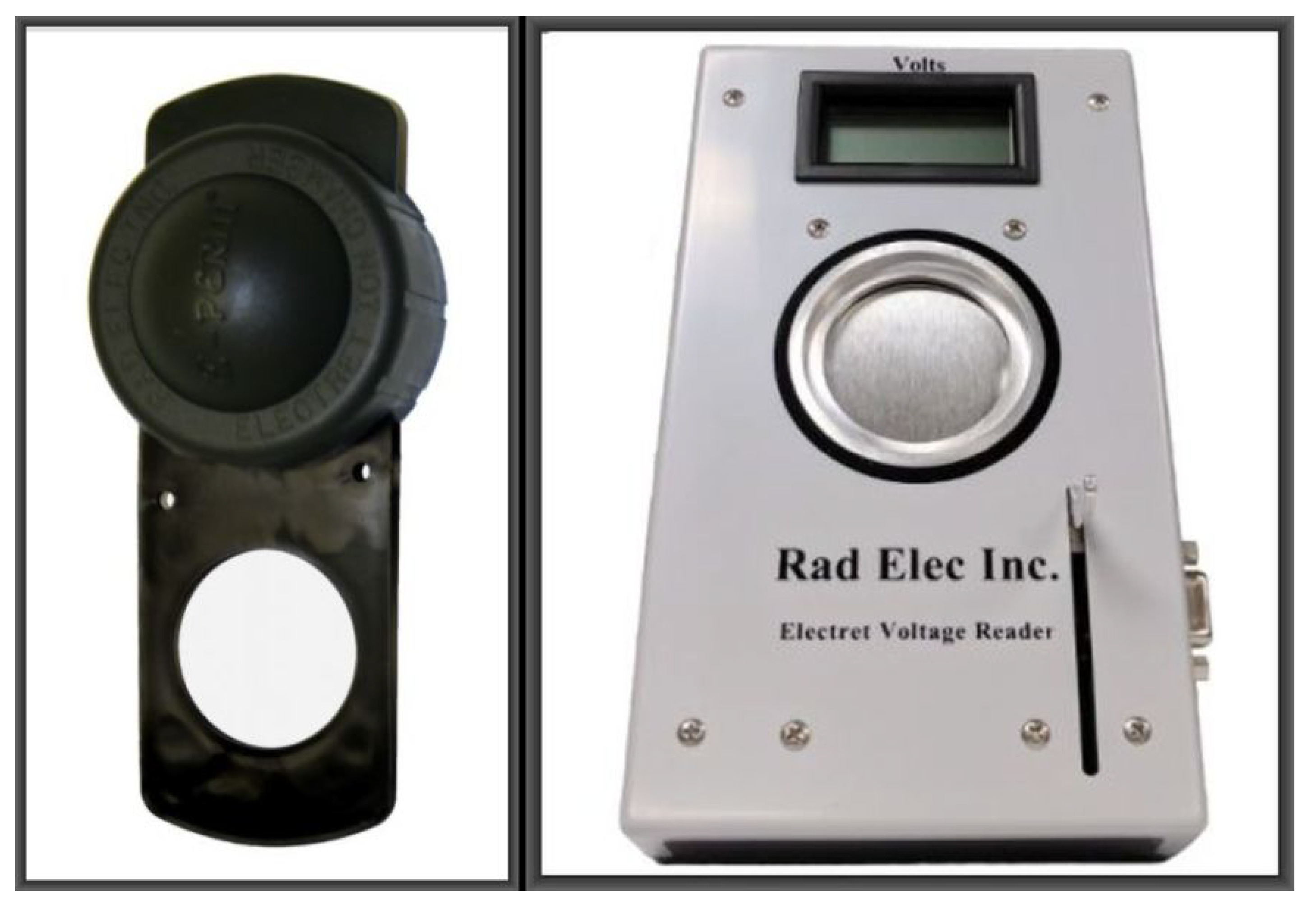
3.1. Passive Radon Detectors
We present results from 36 passive detectors deployed in 23 different neighbourhoods, focusing on parameter estimation, exploratory data visualisation and simulations for replicating crucial parameters and patterns of radon variations.
Table 3 provides summary statistics for the two variables—number of days and concentrations. With the
radon mean at 64.56, the average variation of 39.25 is rather high. Of particular interest was the strong inverse relationship between
radon concentrations and
uncertainity (61%). While this strong correlation does not necessarily mean we attribute
radon concentrations to uncertainty, it highlights the need for further investigations into this detection method. Each device was deployed for at least three months and some remained on site for up to almost nine months. Implicitly, two devices deployed, one for a month and another for six months, are likely to yield approximately readings. Furthermore, the inverse relationship between
radon and
endvolt suggests that the longer the device remains deployed, the more the readings depend on the initial voltage, suggesting further that there is no benefit of long deployment. It is therefore reasonable to focus on
particularly on how
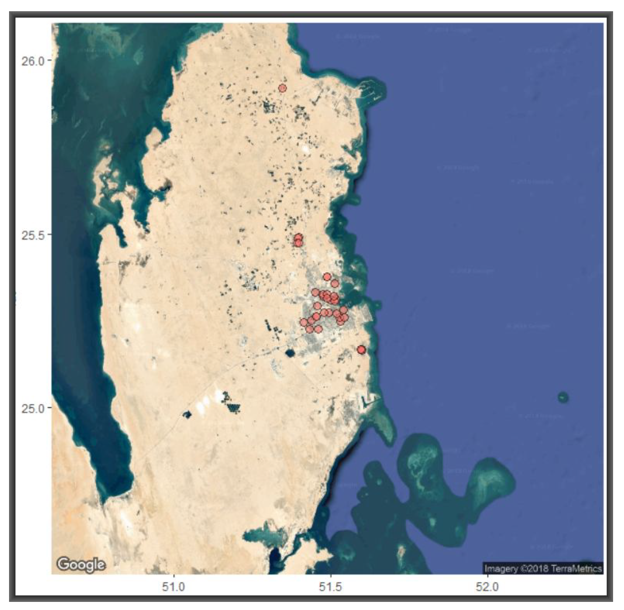
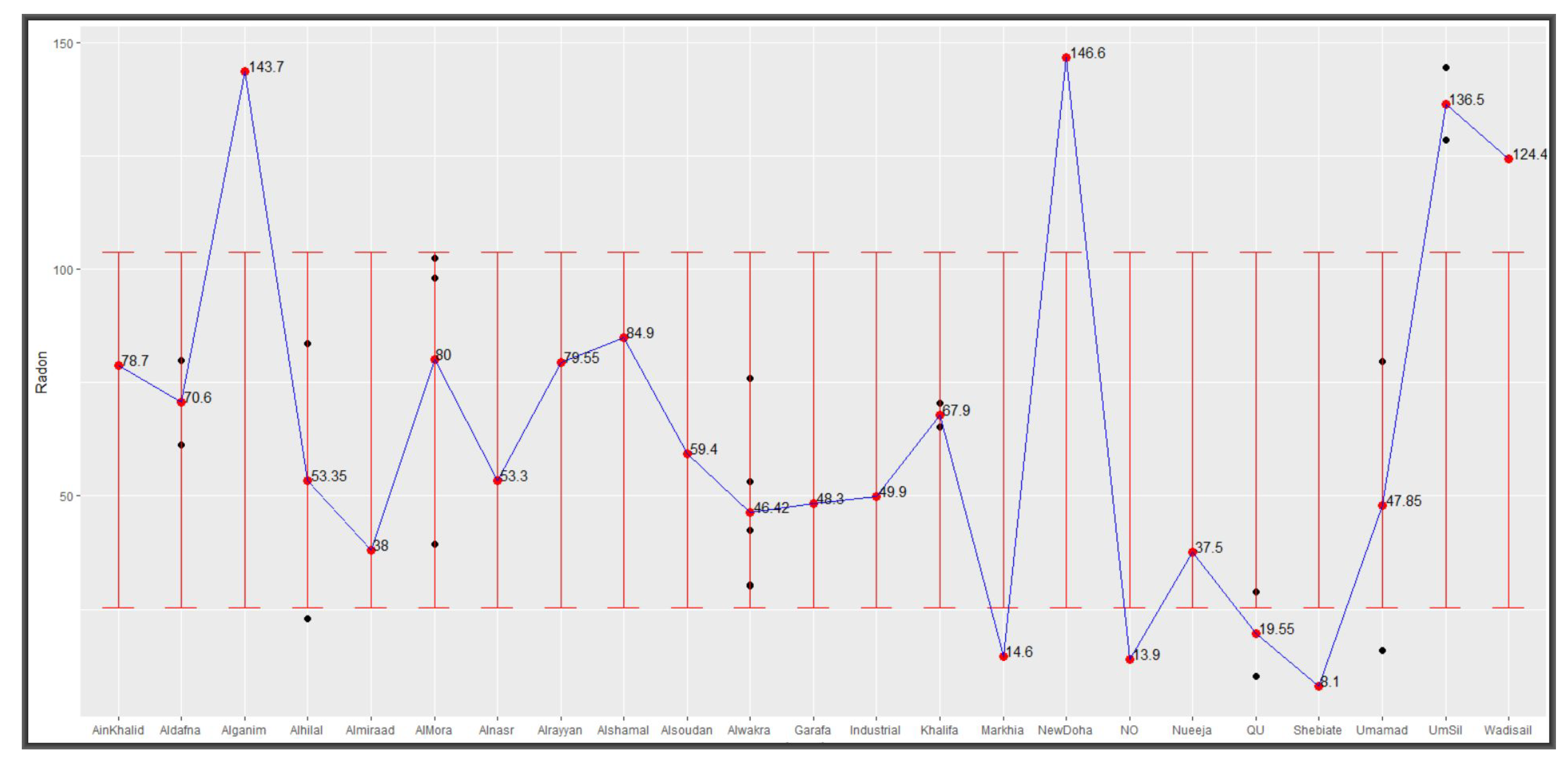
radon concentrations from various locations vary around these parameters. The black and red dots in
Figure 6 show levels of radon concentrations as collected from devices deployed in various locations in and around Doha and their average respectively. Added error bars, based on
and
, show 8 out of the 23 test centres with averages outside the variation interval but all being within Qatar’s acceptable limit of 148 Bq/m
In our final analyses, we explore
radon variations around these parameters.
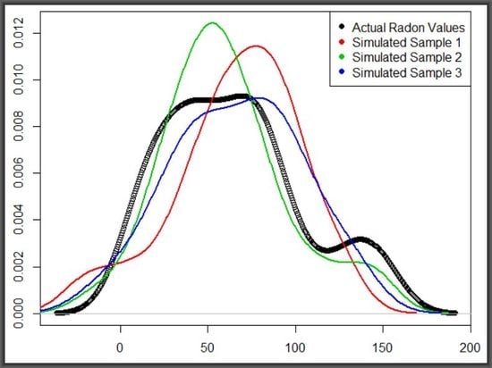
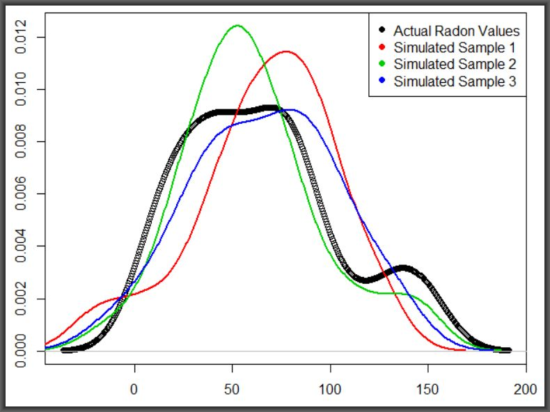
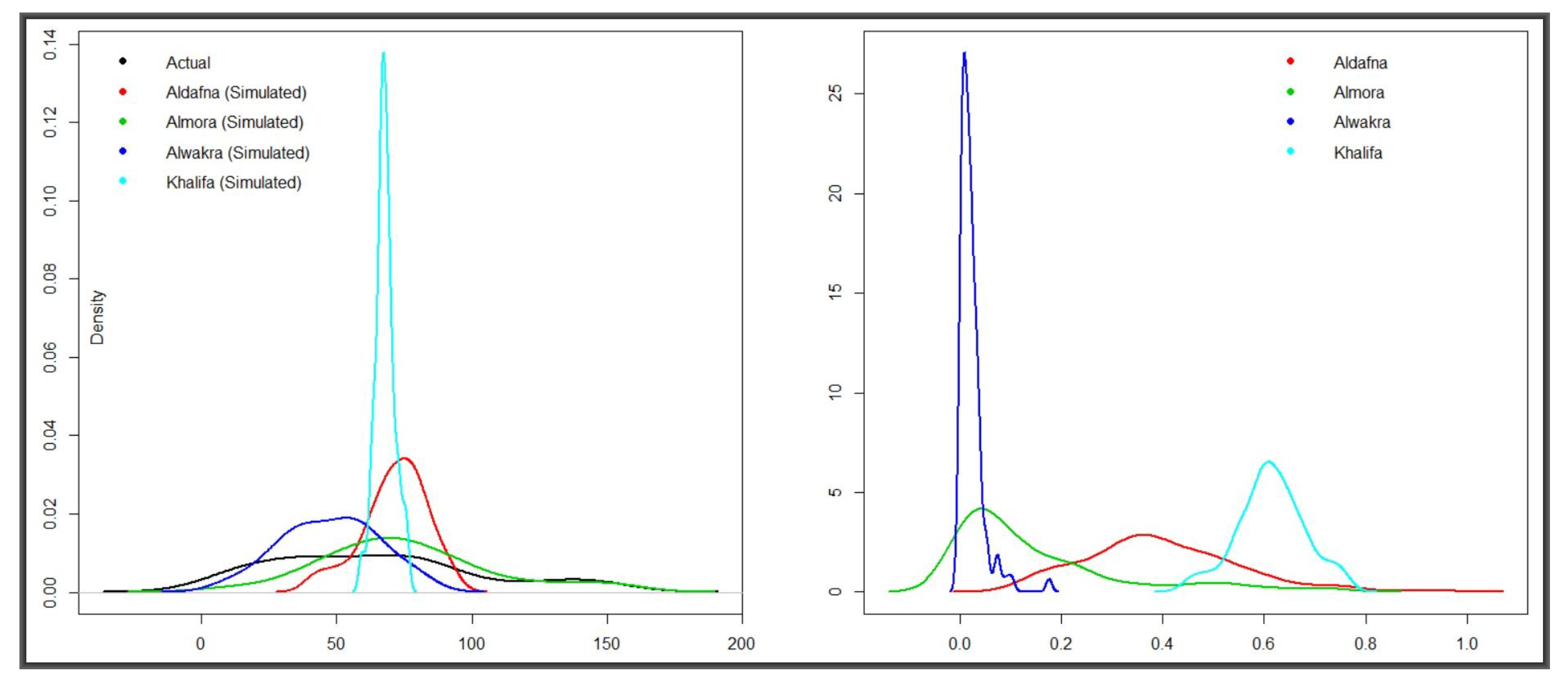
With the exception of Alwakra, which was host to four passive detectors, each of the remaining 35 Doha neighbourhoods had either one or two and with radon concentrations dependent on two parameters, the data sources were constrained. These circumstances provided a motivation for simulating more data to mimick known radon distributions across the neighbourhoods in order to provide a calibrating effect on the detection method. Thus, four neighbourhoods, with meaningful
were selected for data simulation and comparison based on these parameters. The two panels in
Figure 7 are results of
t-tests for similarity between the overall mean of the 36 locations and that of each of the four test centres. They represent hundreds of simulations of random normal values with mean and standard deviations of the data collected from the centres—i.e., simulated values on the left-hand side and the corresponding
p-values on the right. That is, five hundred sample replications were generated and tested for similarity to the overall radon concentration vector. Data from Aldafna and Khalifa exhibited huge departure from the mean, at the 95% level of confidence while only 37% and 10% from Almora and Alwakra, respectively, fell within the acceptable range.
3.2. Active Radon Detectors
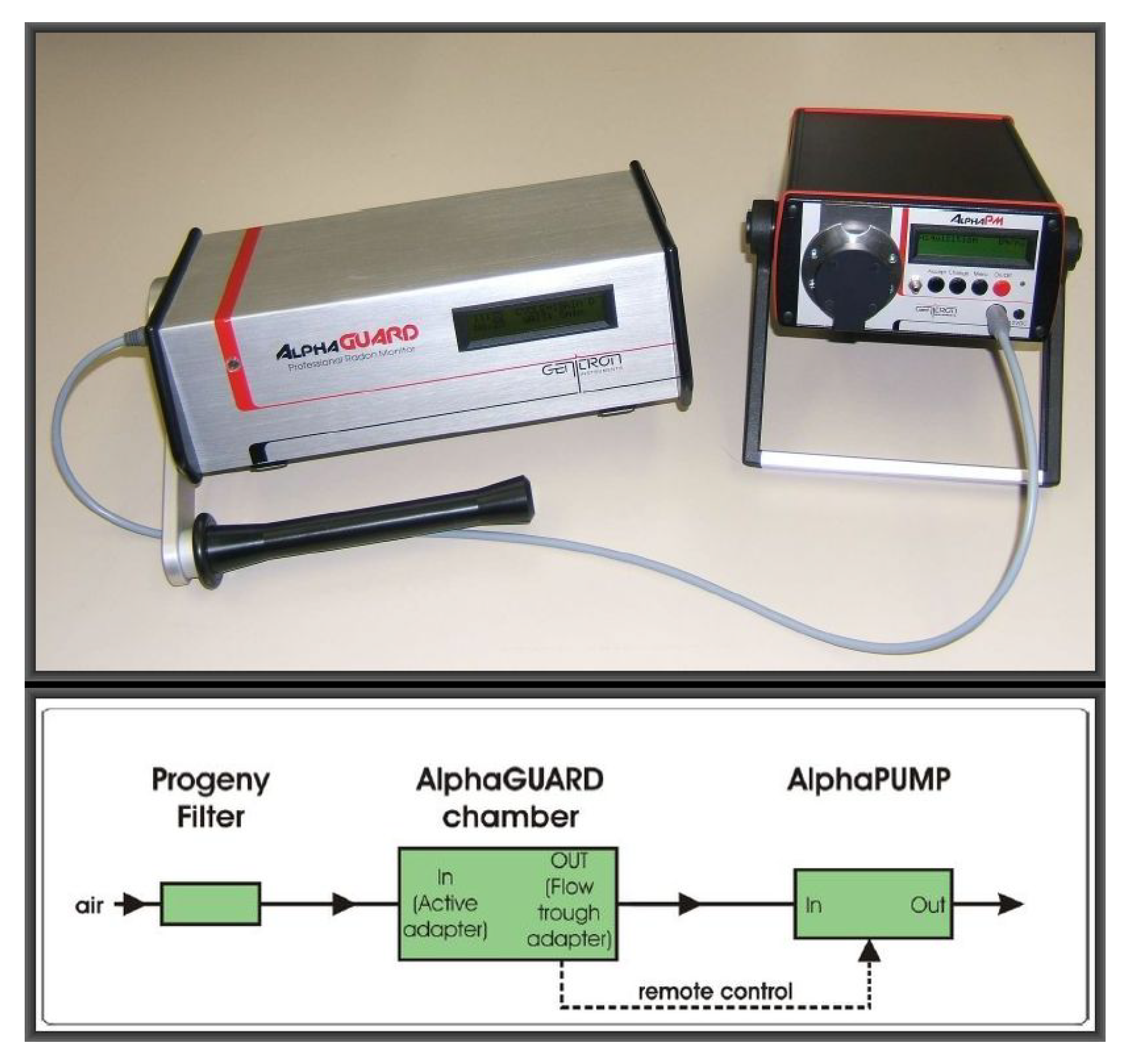
This section presents results from the data captured by the
Alpha Guard active system—a total of 4843 observations on six variables, as summarised in
Table 2. The overall range of radon values generated by
Alpha Guard is very different from the range we saw in
Section 3.1—a variation that is attributable to the equipment used.
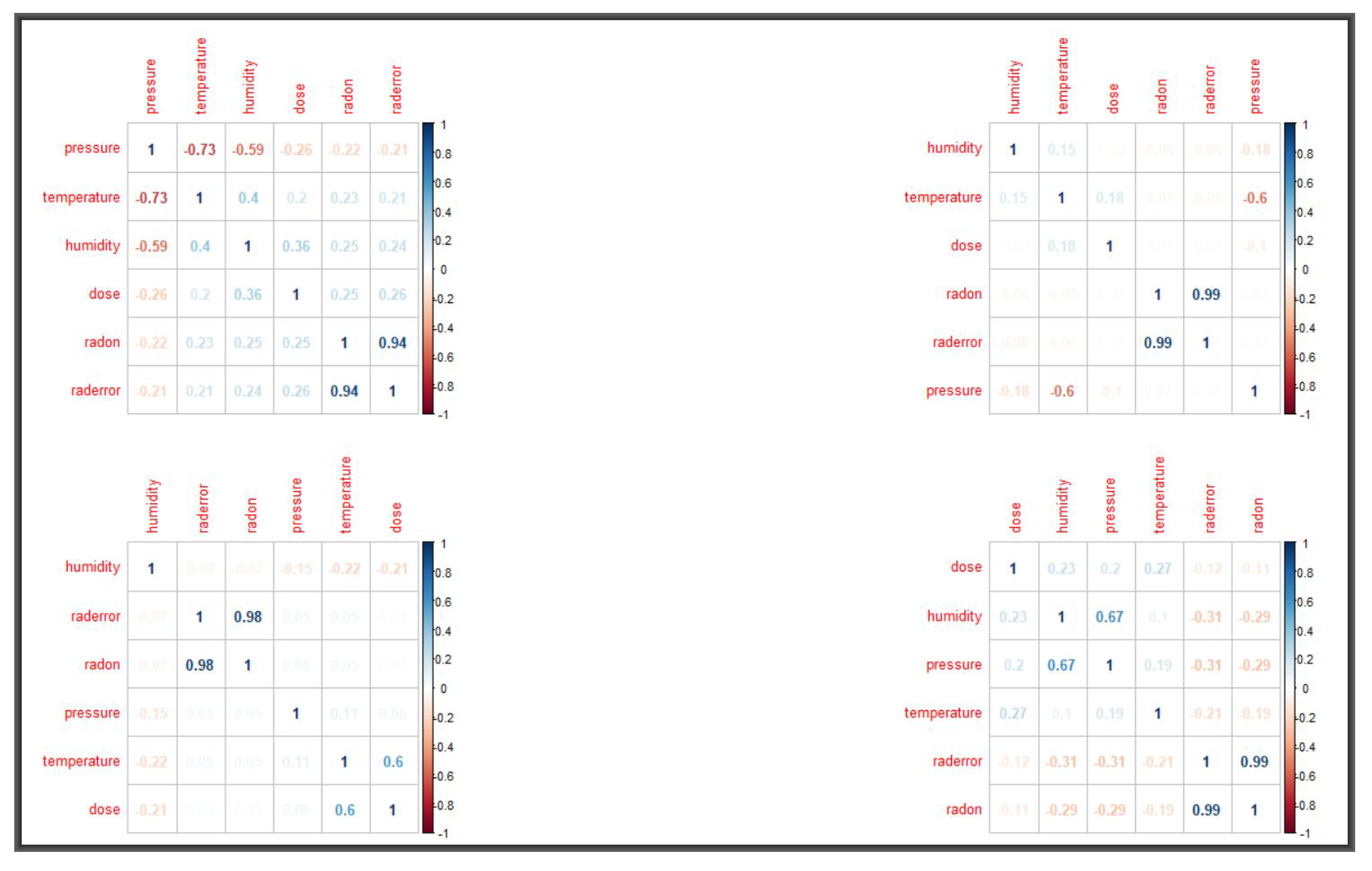
Table 4 shows summaries of the active readings for the months of January 2016 and September 2017. Used in the analyses below are also radon readings for the months of April, May, June, July and August of 2017. Variable correlations are given in
Figure 8 and, as it can be seen, radon does not appear to correlate with any of the meteorological factors. Our final analyses focus on local regression and clustering. In both cases, we aim to determine the optima values for the smoothing parameter and therefore we fit both the
loess() function and
K-means via Algorithm 1.
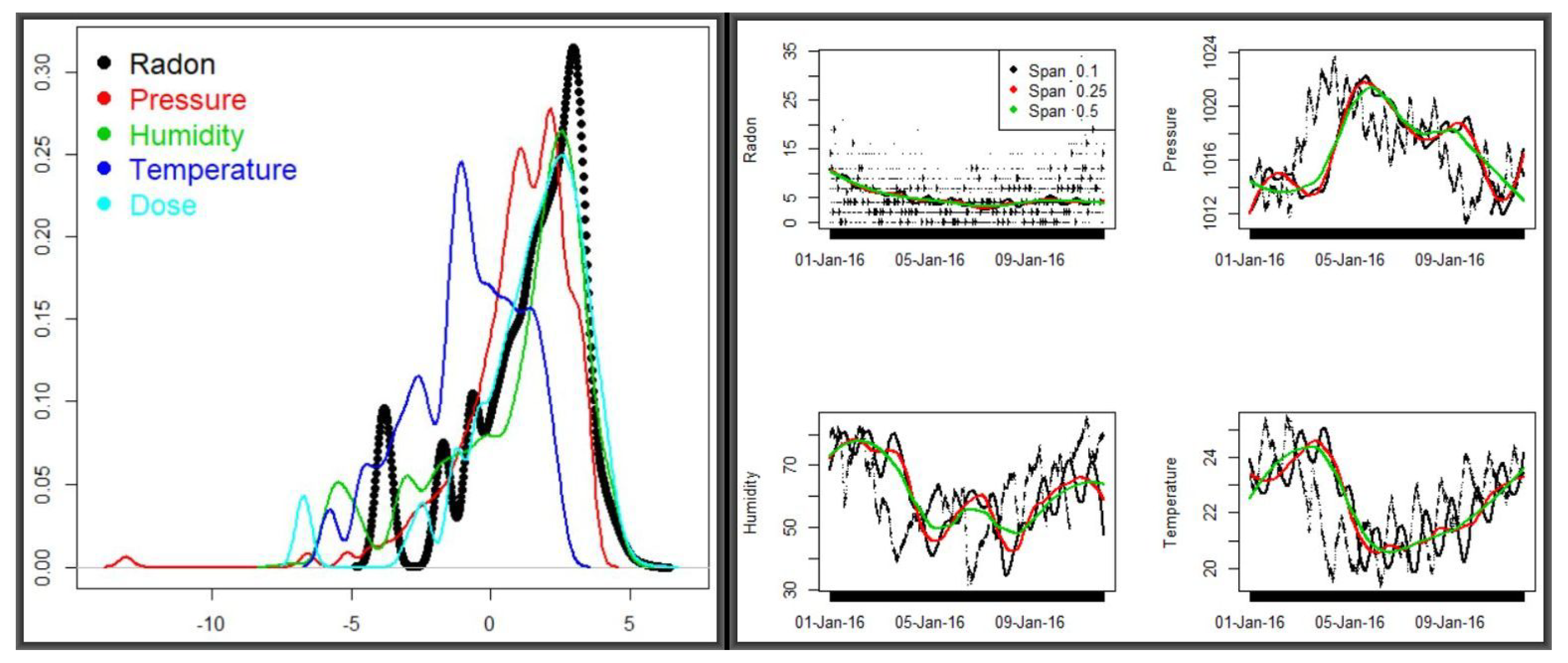
Minimising the error—i.e., the smoothing parameter that minimizes the Sum of Squared Errors (SSE) requires lower values of span—which obviously might lead to spurious peaks. Based on different smoothing parameters, we implemented Algorithm 1 to obtain optimal parameters from the predictions by averaging over multiple span runs.
Figure 9 shows the densities for the five variables in the combined dataset (left panel) and the smoothed predictions of radon and meteorologcal variables for two periods of the year (discussed below). Corresponding descriptive summaries for the
loess smoothing and
predictions of radon and the three meteorological variables—
radon, pressure, humidity and
temperature are provided in
Table 5. These variable means were obtained by iteratively refining a span vector of length 40—from 0.025 to 1 at step 0.025. The vector was input to a
loess function, updating
as in step 13 of Algorithm 1. The three span values yielded the closest estimations to the actual means in
Table 4.
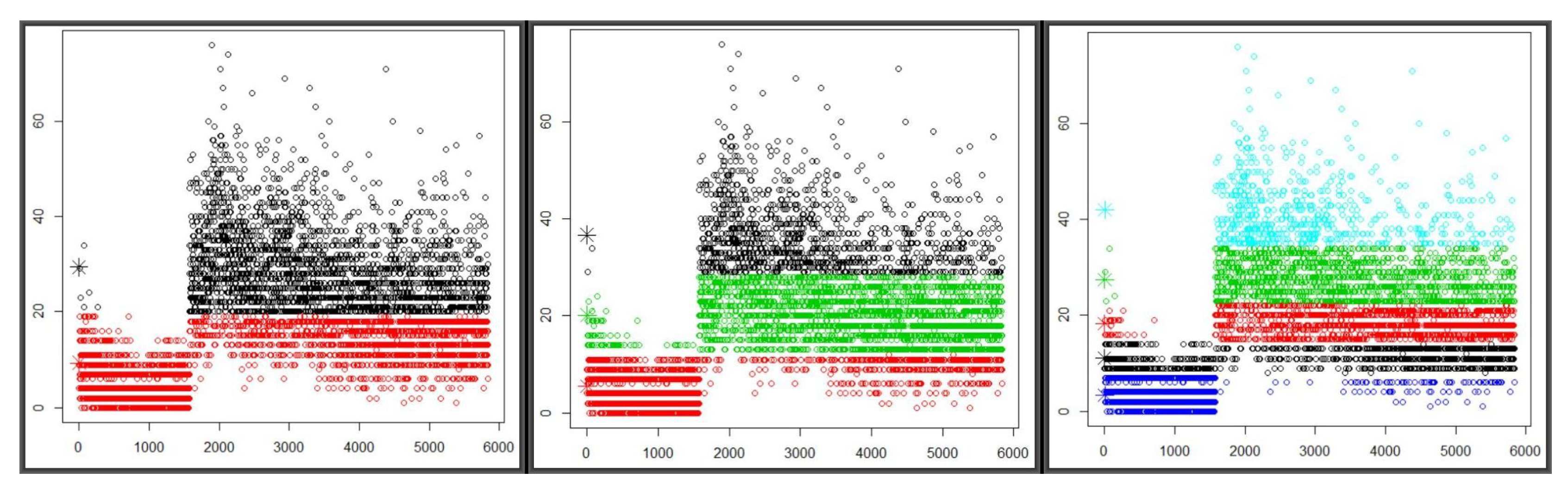
The huge variation of radon concentration between the two periods of year was pronounced throughout the spans—but the fact that there are other variables showing little sensitivity to time variations suggests that there must be other factors affecting radon levels. In the next exposition, we carry out two types of analyses—multiple observational and variable clustering, both running through Algorithm 1, for an indication as to which directions to look further. The three panels in
Figure 10, left to right, show graphical patterns from the
K-Means algorithm on two, three and five centroids, respectively. They are based on
radon readings every ten minutes from 30 December 2015 to Sunday, 10 January 2016, combined with those from Tuesday, 29 August 2017 to Thursday, 28 September 2017. The first chunk has 1576 observations with a mean of 4.87 and standard deviation of 4.15, whereas the second consists of 4263 with a mean and standard deviation of 23.57 and 10.25, respectively. All three panels exhibit a huge gap between the first and second chunks of observations, with the former being characterised by low readings and the early readings of the latter starting with extremely high readings and slowly levelling down in mid-September. It may be plausible to attribute the gap to weather variation—also possibly to the data gap between Monday, 11 January 2016 and Monday, 28 August 2017 as the period covers the last days of winter and the onset of summer.
The search for, and optimal testing of, fitted parameters was via Algorithm 1 from which
Table 6 was generated. The
Welch Two Sample t-test was carried out between the full elements of each cluster and a sample of 100 drawn from it in order to determine the representativeness of the centroids with respect to the overall
radon readings. The samples were generated as random normal with mean and standard deviation equal to those of the cluster and, despite clear separation between the two chunks of data, sample means hugely differed from those of the two clusters.
Table 6 shows that the measure of the goodness of the
K-Means classification—i.e., the decomposition of deviance in deviance between and within clusters grows with the number of clusters. Notice that all but two centroids are highly significant. However, the higher the ratio, the higher the cohesion, and we must always be careful as that may lead to over-fitting.
One in the three cluster setting was consistently in agreement with the overall cluster mean, whereas, in the five-cluster setting, this happened only once in 150 runs. It is reasonable to go for three natural clusters in this dataset, but it is imperative to explore factors that may have led to this variation.
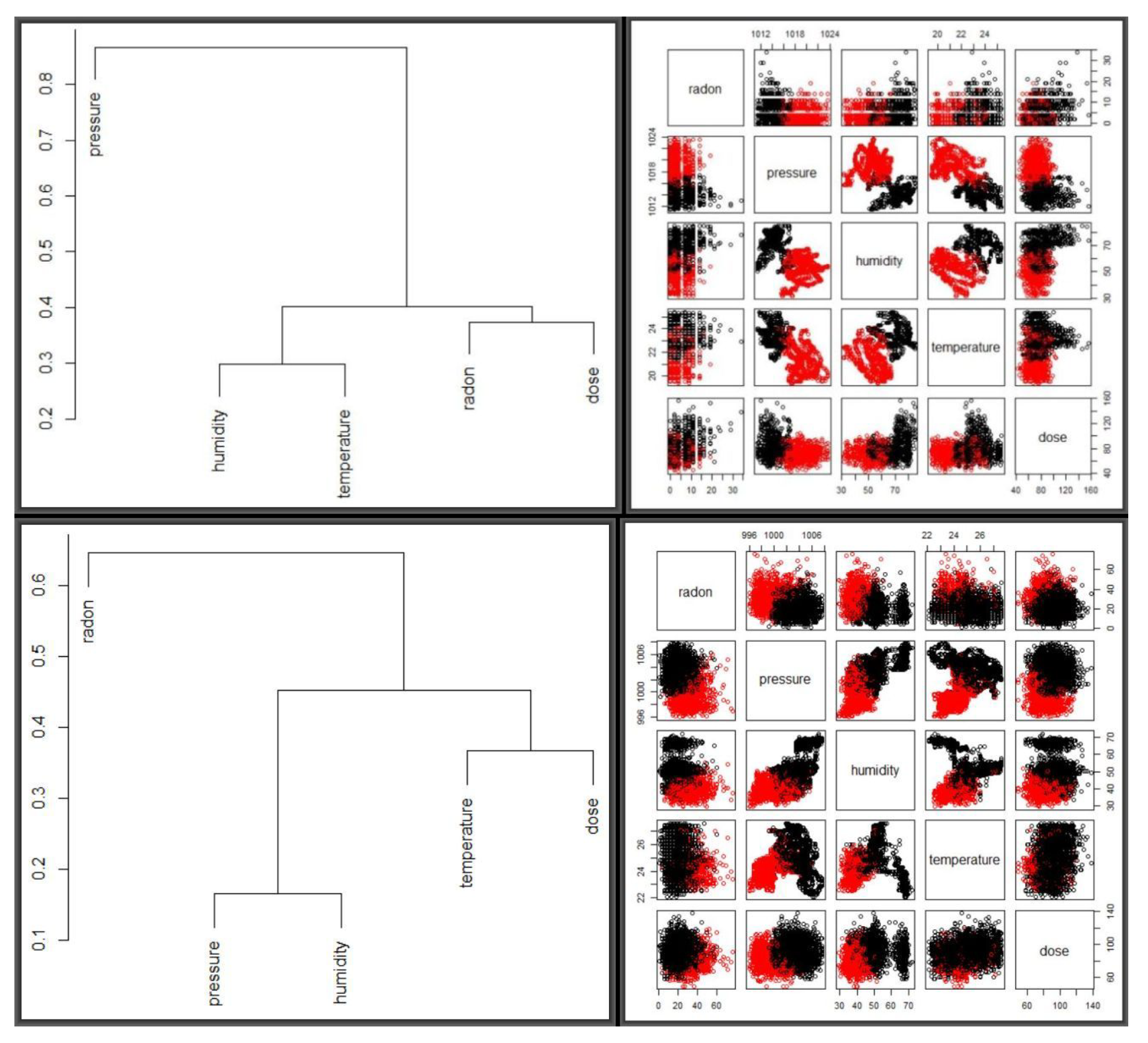
Figure 11 shows dendograms and and optimal two clusters for the two periods, side by side, scaled by the mean and standard deviation, as shown in
Table 7. The top two panels represent the January 2016 period while the bottom two correspond to September 2017.
For optimisation, the
K-means algorithm was repeatedly fitted via Algorithm 1 compared based on scaling methods and cluster numbers and yielding two optimal clusters with clearer separation observed for September 2017 than for January 2016. Columns 2, 3 and 4 of
Table 7 were obtained from hundreds of candidate simulations, based on eight scaling methods and cluster numbers between 2 and 15. For both periods, scaling about the mean and standard deviation yielded the best results, with tests similar to those in
Table 6 suggesting that three clusters were optimal for both periods. A larger number of clusters yielded very high
between to
total variation, which, as we explain below, is susceptible to over-fitting. Finally, the
mclust [
21] also performed better on the data with Algorithm 1 than without.
For both sets of results presented in
Table 6 and
Table 7, it is worth noting that the algorithm updates cluster centers, allocating observation as it moves until the set condition is met or the change of within-cluster sum of squares in successive iterations becomes insignificant. Updated cluster centers are associated with a measure of the total variance in the dataset that is explained by the clustering. The goal is to minimize the within cluster variation and maximize the between-cluster variation dispersion. However, while we want a higher proportion of
between to
total variation—as it represents the variance in the data set that is explained by the clustering—i.e., a reduction in sums of squares in percentage, we do not want to overfit the data, as this is what is potentially likely with cluster numbers 5 and above.


