Temporal Statistical Analysis of Degree Distributions in an Undirected Landline Phone Call Network Graph Series


Abstract
:1. Introduction
2. Materials and Methods
2.1. Data Preparation
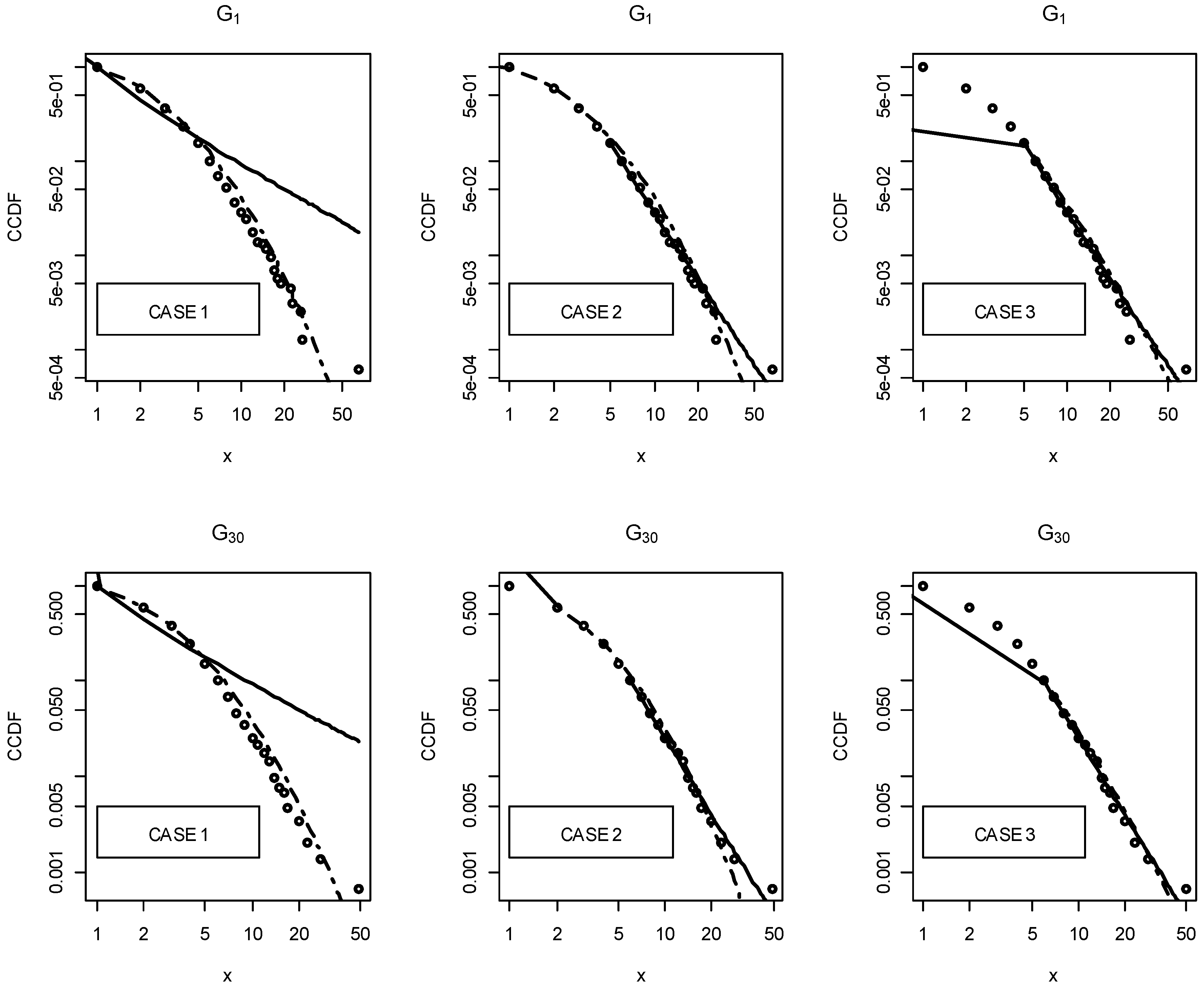
2.2. Temporal Statistical Analysis
- Case 1: the fitting made from 1;
- Case 2: the fitting made from the estimated of each distribution;
- Case 3: the fitting made from the where both distributions are plausible.
3. Results
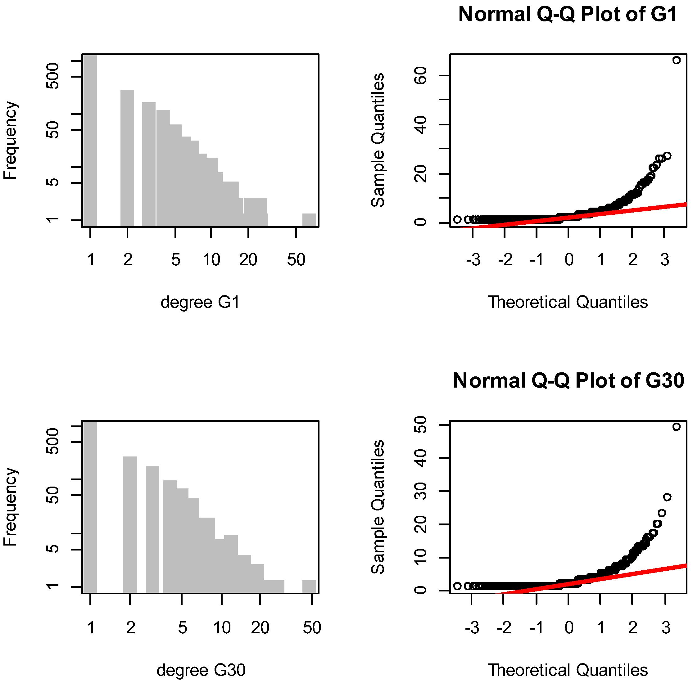
3.1. Descriptive Analysis of Degree Values
- the degree sequence is unimodal;
- the mode is 1;
- mean median mode;
- the peak of the data is on the left and the right tail is longer;
- skewness is greater than 1;
- kurtosis is greater than 3.
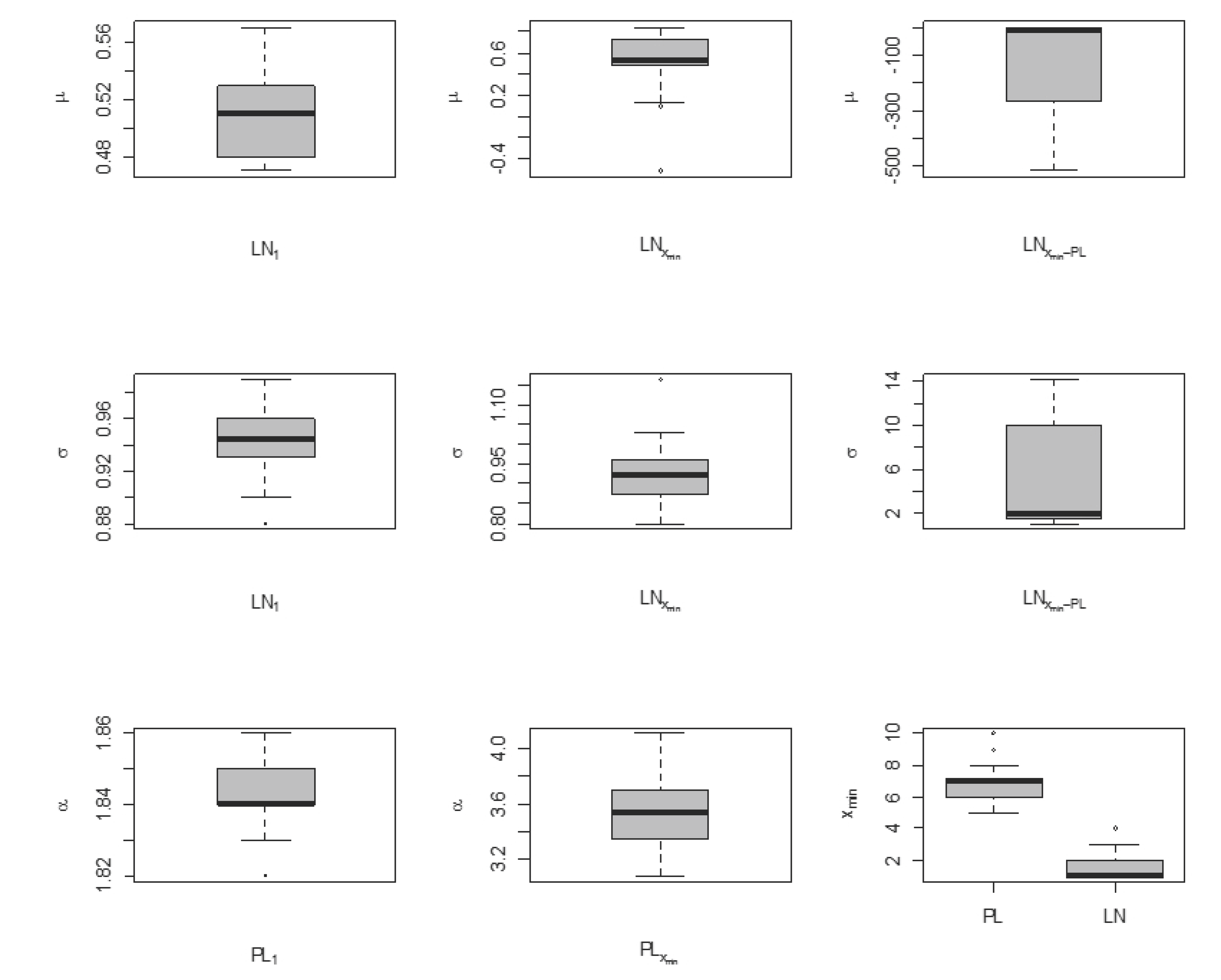
3.2. Statistical Analysis of Fitted Distributions
- : In all three cases, does not come from a normal distribution, and its shape is described as follows:
- Case 1: approximately symmetric and platykurtic;
- Case 2: highly negative skewed and leptokurtic;
- Case 3: highly negative skewed and platykurtic.
- : In Cases 1 and 2, based on the Shapiro-Wilk test, the normal distribution was not rejected, but it was in Case 3. The shape of the distribution is described as follows:
- Case 1: approximately symmetric and platykurtic;
- Case 2: moderately skewed and platykurtic;
- Case 3: moderately skewed and platykurtic.
4. Discussion
Supplementary Materials
Conflicts of Interest
References
- Nanavati, A.-A.; Singh, R.; Chakraborty, D.; Dasgupta, K.; Mukherjea, S.; Das, G.; Gurumurthy, S.; Joshi, A. Analyzing the Structure and Evolution of Massive Telecom Graphs. IEEE Trans. Knowl. Data Eng. 2008, 20, 703–718. [Google Scholar] [CrossRef]
- Nanavati, A.-A.; Gurumurthy, G.-D.; Das, G.; Chakraborty, D.; Dasgupta, K.; Mukherjea, S.; Joshi, A. On the Structural Properties of Massive Telecom Call Graphs: Finding and Implications. In Proceedings of the 15th ACM International Conference on Information and Knowledge Management, CIKM’06, Arlington, VA, USA, 6–11 November 2006. [Google Scholar]
- Seshadri, M.; Machiraju, S.; Sridharan, A.; Bolot, J.; Faloutsos, Ch.; Leskovec, J. Mobile Call Graphs: Beyond Power-Law and Lognormal Distributions. In Proceedings of the 14th ACM SIGKDD International Conference on Knowledge Discovery and Data Mining, KDD’08, Las Vegas, NV, USA, 24–27 August 2008. [Google Scholar]
- Dong, Z.-B.; Song, G.-J.; Xie, K.-Q.; Wang, J.-Y. An Experimental Study of Large-Scale Mobile Social Network. In Proceedings of the 18th International Conference on World Wide Web, WWW 2009, Madrid, Spain, 20–24 April 2009. [Google Scholar]
- Noka (Jani), E.; Hoxha, F. Comparative Analysis of the Structural and Weighted Properties in Albanian Social Networks. J. Multidiscip. Eng. Sci. Technol. 2016, 3, 4505–4509. [Google Scholar]
- Onnela, J.-P.; Saramäki, J.; Hyvӧven, J.; Szabó, G.; Lazer, D.; Kaski, K.; Kertész, J.; Barabási, A.-L. Structure and Tie Strengths in Mobile Communication Networks. Proc. Natl. Acad. Sci. USA 2007, 104, 7332–7336. [Google Scholar] [CrossRef] [PubMed]
- Onnela, J.-P.; Saramäki, J.; Hyvӧnen, J.; Szabó, G.; Argollo de Mendez, M.; Kaski, K.; Barabási, A.-L.; Kertész, J. Analysis of a large-scale weighted network of one-to-one human communication. New J. Phys. 2007, 9, 179. [Google Scholar] [CrossRef]
- Aiello, W.; Chung, F.; Lu, L. A random graph model for massive graphs. In Proceedings of the 32nd Annual ACM Symposium on Theory of Computing, New York, NY, USA, 21–23 May 2000. [Google Scholar]
- Aiello, W.; Chung, F.; Lu, L. A random graph model for power law graphs. Exp. Math. 2001, 10, 53–66. [Google Scholar] [CrossRef]
- Gjermëni, O.; Ramosaço, M.; Zotaj, D. Power-Law versus Lognormal Distribution in a Phone Call Network Graph. In Proceedings of the International Conference on Application of Information and Communication Technology and Statistics in Economy and Education (ICAICTSEE), Sofia, Bulgaria, 13–14 November 2015. [Google Scholar]
- Cortes, C.; Pregibon, D.; Volinsky, C. Communities of Interest. In Advances in Intelligent Data Analysis; Springer: Berlin, Germany, 2001; pp. 105–114. [Google Scholar]
- Ye, Q.; Zhu, T.; Hu, D.; Wu, B.; Du, N.; Wang, B. Cell Phone Mini Challenge Award: Social Network Accuracy—Exploring Temporal Communication in Mobile Call Graphs. In Proceedings of the IEEE Symposium on Visual Analytics Science and Technology, Columbus, OH, USA, 19–24 October 2008. [Google Scholar]
- Newman, M.-E.-J. The Structure and Function of Complex Networks. SIAM Rev. 2003, 45, 167–256. [Google Scholar] [CrossRef]
- Royston, P. An extension of Shapiro and Wilk’s W test for normality to large samples. Appl. Stat. 1982, 31, 115–124. [Google Scholar] [CrossRef]
- Royston, P. Algorithm AS 181: The W test for Normality. Appl. Stat. 1982, 31, 176–180. [Google Scholar] [CrossRef]
- Royston, P. Remark AS R94: A remark on Algorithm AS 181: The W test for normality. Appl. Stat. 1995, 44, 547–551. [Google Scholar] [CrossRef]
- Bulmer, M.-G. Principles of Statistics; Dover Publications: New York, NY, USA, 1979. [Google Scholar]
- Balanda, K.-P.; MacGillivray, H.-L. Kurtosis: A Critical Review. Am. Stat. 1988, 42, 111–119. [Google Scholar]
- Hanusz, Z.; Tarasińska, J. Impact of Alternative Distributions on Quantile–Quantile Normality Plot. Colloq. Biom. 2015, 45, 67–78. [Google Scholar]
- Foss, S.; Korshunov, D.; Zachary, S. An Introduction to Heavy-Tailed and Subexponential Distributions; Springer Science+Business Media: New York, NY, USA, 2013. [Google Scholar]
- Clauset, A.; Shalizi, C.-R.; Newman, M.-E.-J. Power-Law Distributions in Empirical Data. SIAM Rev. 2009, 51, 661–703. [Google Scholar] [CrossRef]
- Clauset, A.; Shalizi, C.-R.; Newman, M.-E.-J. Power-Law Distribution in Empirical Data. Available online: http://tuvalu.santafe.edu/~aaronc/powerlaws/ (accessed on 7 June 2007).
- Shim, J. Toward a more nuanced understanding of long-tail. J. Bus. Ventur. Insights 2016, 6, 21–27. [Google Scholar] [CrossRef]
- Vuong, Q.-H. Likelihood ratio tests for model selection and non-nested hypothesis. Econometrica 1989, 57, 307–333. [Google Scholar] [CrossRef]
- Rmetrics Core Team. R: A Language and Environment for Statistical Computing. Available online: https://www.R-project.org/ (accessed on 21 April 2017).
- Gillespie, C.-S. Fitting Heavy Tailed Distributions: The powerRlaw Package. J. Stat. Softw. 2015, 64, 1–16. [Google Scholar] [CrossRef]
- Rmetrics Core Team; Wuertz, D.; Setz, T.; Chalabi, Y. fBasics: Rmetrics-Markets and Basic Statistics; R package 3011.87. Available online: https://CRAN.R-project.org/package=fBasics (accessed on 29 October 2014).
- Csardi, G. Igraphdata: A Collection of Network Data Sets for the ‘igraph’ Package. Available online: https://CRAN.R-project.org/package=igraphdata (accessed on 13 July 2015).
- Csardi, G.; Nepusz, T. The igraph software package for complex network research. InterJournal 2006, 1695, 1–9. [Google Scholar]

| Authors | Data | Time | Directed | Mutual | Simplified | Weighted |
|---|---|---|---|---|---|---|
| Nanavati et al. [1,2] | mobile | 1 w, 1 m | yes | no | yes | no |
| Seshadri et al. [3] | mobile | 2 m | no | yes | yes | yes |
| Dong et al. [4] | mobile | 1 m | no | no | yes | no |
| Onnela et al. [6,7] | mobile | 18 w | no | Both (yes, no) | - | yes |
| Ye et al. [12] | mobile | 10 d | yes | no | no | no |
| Noka (Jani) & Hoxha [5] | mobile (calls, SMS) | 1 m | no | yes | - | yes |
| Aiello et al. [8,9] | landline | 1 d | yes | no | no | no |
| Gjermëni & Ramosaco [10] | landline | 1 m | Both (yes, no) | no | yes | yes |
| Basic Stats | ||
|---|---|---|
| Minimum | 1 | 1 |
| First Quartile | 1 | 1 |
| Median | 2 | 2 |
| Third Quartile | 3 | 3 |
| Maximum | 66 | 49 |
| Mean | 2.79 | 2.77 |
| Skewness | 7.25 | 5.77 |
| Kurtosis | 108.41 | 57.91 |
| Mode | 1 | 1 |
| n | PL | |||
|---|---|---|---|---|
| 1 | 1597 | 5 (245) | 3.27 | 0.02 (0.665) |
| 2 | 1428 | 6 (153) | 3.95 | 0.04 (0.274) |
| 3 | 1561 | 5 (276) | 3.07 | 0.03 (0.195) |
| 4 | 1534 | 8 (108) | 3.78 | 0.03 (0.813) |
| 5 | 1522 | 7 (117) | 3.64 | 0.03 (0.459) |
| 6 | 1530 | 7 (132) | 3.49 | 0.03 (0.509) |
| 7 | 1531 | 9 (74) | 3.66 | 0.02 (0.895) |
| 8 | 1560 | 6 (199) | 3.37 | 0.03 (0.388) |
| 9 | 1487 | 7 (110) | 3.64 | 0.03 (0.801) |
| 10 | 1564 | 9 (76) | 3.69 | 0.03 (0.846) |
| 11 | 1545 | 7 (131) | 3.67 | 0.03 (0.819) |
| 12 | 1531 | 8 (97) | 3.46 | 0.04 (0.274) |
| 13 | 1547 | 7 (121) | 3.58 | 0.04 (0.359) |
| 14 | 1552 | 7 (133) | 3.69 | 0.02 (0.988) |
| 15 | 1555 | 9 (79) | 3.88 | 0.04 (0.569) |
| 16 | 1554 | 8 (90) | 4.11 | 0.02 (0.992) |
| 17 | 1555 | 6 (195) | 3.43 | 0.03 (0.483) |
| 18 | 1560 | 7 (126) | 3.42 | 0.03 (0.653) |
| 19 | 1494 | 5 (235) | 3.24 | 0.03 (0.204) |
| 20 | 1568 | 5 (257) | 3.31 | 0.04 (0.062) |
| 21 | 1523 | 7 (137) | 3.61 | 0.04 (0.192) |
| 22 | 1505 | 7 (130) | 3.49 | 0.03 (0.489) |
| 23 | 1479 | 7 (117) | 3.87 | 0.04 (0.377) |
| 24 | 1512 | 5 (247) | 3.14 | 0.02 (0.682) |
| 25 | 1559 | 5 (260) | 3.15 | 0.03 (0.204) |
| 26 | 1545 | 10 (60) | 3.78 | 0.03 (0.702) |
| 27 | 1530 | 6 (163) | 3.35 | 0.04 (0.130) |
| 28 | 1505 | 6 (176) | 3.18 | 0.04 (0.253) |
| 29 | 1524 | 7 (127) | 3.49 | 0.03 (0.528) |
| 30 | 1472 | 6 (151) | 3.58 | 0.02 (0.819) |
| n | LN | ||||
|---|---|---|---|---|---|
| 1 | 1597 | 1 (1597) | 0.48 | 0.93 | 0.01 (0.196) |
| 2 | 1428 | 1 (1428) | 0.52 | 0.88 | 0.01 (0.016) |
| 3 | 1561 | 3 (619) | 0.38 | 0.99 | 0.01 (0.793) |
| 4 | 1534 | 2 (906) | 0.83 | 0.84 | 0.01 (0.239) |
| 5 | 1522 | 2 (913) | 0.79 | 0.81 | 0.01 (0.426) |
| 6 | 1530 | 1 (1530) | 0.54 | 0.93 | 0.01 (0.184) |
| 7 | 1531 | 4 (400) | 0.12 | 1.03 | 0.01 (0.703) |
| 8 | 1560 | 1 (1560) | 0.56 | 0.95 | 0.01 (0.251) |
| 9 | 1487 | 1 (1487) | 0.52 | 0.90 | 0.00 (0.948) |
| 10 | 1564 | 1 (1564) | 0.50 | 0.95 | 0.00 (0.876) |
| 11 | 1545 | 2 (932) | 0.71 | 0.86 | 0.01 (0.424) |
| 12 | 1531 | 1 (1531) | 0.49 | 0.96 | 0.01 (0.037) |
| 13 | 1547 | 1 (1547) | 0.53 | 0.92 | 0.01 (0.653) |
| 14 | 1552 | 2 (949) | 0.84 | 0.81 | 0.01 (0.247) |
| 15 | 1555 | 1 (1555) | 0.47 | 0.97 | 0.00 (0.969) |
| 16 | 1554 | 2 (910) | 0.78 | 0.81 | 0.01 (0.556) |
| 17 | 1555 | 2 (926) | 0.72 | 0.88 | 0.01 (0.413) |
| 18 | 1560 | 4 (397) | −0.52 | 1.16 | 0.01 (0.895) |
| 19 | 1494 | 1 (1494) | 0.51 | 0.92 | 0.00 (0.898) |
| 20 | 1568 | 1 (1568) | 0.56 | 0.90 | 0.01 (0.162) |
| 21 | 1523 | 1 (1523) | 0.57 | 0.93 | 0.02 (0.009) |
| 22 | 1505 | 2 (894) | 0.74 | 0.87 | 0.01 (0.464) |
| 23 | 1479 | 2 (859) | 0.81 | 0.80 | 0.01 (0.223) |
| 24 | 1512 | 1 (1512) | 0.5 | 0.95 | 0.01 (0.622) |
| 25 | 1559 | 1 (1559) | 0.48 | 0.96 | 0.01 (0.379) |
| 26 | 1545 | 1 (1545) | 0.47 | 0.99 | 0.01 (0.467) |
| 27 | 1530 | 3 (577) | 0.10 | 1.03 | 0.01 (0.871) |
| 28 | 1505 | 1 (1505) | 0.52 | 0.95 | 0.01 (0.590) |
| 29 | 1524 | 2 (917) | 0.66 | 0.89 | 0.01 (0.740) |
| 30 | 1472 | 2 (882) | 0.74 | 0.80 | 0.01 (0.488) |
| LN Conditioned by PL | LN vs. PL | ||||
|---|---|---|---|---|---|
| 1 | 5 (245) | −3.36 | 1.59 | 0.516 | 0.606 |
| 2 | - | - | - | - | - |
| 3 | 5 (276) | −0.02 | 1.08 | 1.232 | 0.218 |
| 4 | 8 (108) | −490.96 | 13.36 | 0.268 | 0.788 |
| 5 | 7 (117) | −48.44 | 4.40 | 0.087 | 0.931 |
| 6 | 7 (132) | −5.14 | 1.77 | 0.328 | 0.743 |
| 7 | 9 (74) | −10.23 | 2.22 | 0.114 | 0.909 |
| 8 | 6 (199) | −7.20 | 2.03 | 0.253 | 0.8 |
| 9 | 7 (110) | −505.22 | 13.89 | -0.007 | 0.994 |
| 10 | 9 (76) | −512.04 | 13.85 | 0.424 | 0.671 |
| 11 | 7 (131) | −519.53 | 14.02 | 0.459 | 0.647 |
| 12 | - | - | - | - | - |
| 13 | 7 (121) | −123.13 | 7.00 | 0.342 | 0.732 |
| 14 | 7 (133) | −266.38 | 10.02 | 0.052 | 0.958 |
| 15 | 9 (79) | −20.99 | 2.88 | 0.063 | 0.95 |
| 16 | 8 (90) | −440.36 | 11.97 | −0.032 | 0.975 |
| 17 | 6 (195) | −2.79 | 1.48 | 0.447 | 0.655 |
| 18 | 7 (126) | −1.35 | 1.29 | 0.458 | 0.647 |
| 19 | 5 (235) | −0.21 | 1.07 | 0.928 | 0.353 |
| 20 | - | - | - | - | - |
| 21 | - | - | - | - | - |
| 22 | 7 (130) | −2.56 | 1.45 | 0.361 | 0.718 |
| 23 | 7 (117) | −5.83 | 1.71 | 0.243 | 0.808 |
| 24 | 5 (247) | −6.89 | 2.09 | 0.399 | 0.69 |
| 25 | 5 (260) | −0.66 | 1.19 | 0.855 | 0.393 |
| 26 | 10 (60) | −490.04 | 13.32 | 0.081 | 0.936 |
| 27 | 6 (163) | −3.12 | 1.55 | 0.0378 | 0.705 |
| 28 | 6 (176) | −0.26 | 1.14 | 0.772 | 0.44 |
| 29 | 7 (127) | −6.08 | 1.88 | 0.185 | 0.85 |
| 30 | 6 (151) | −2.60 | 1.40 | 0.411 | 0.68 |
| Statistics | ||||||
|---|---|---|---|---|---|---|
| Minimum | 0.47 | −0.52 | −519.53 | 0.88 | 0.80 | 1.07 |
| First Quartile | 0.48 | 0.48 | −230.57 | 0.93 | 0.87 | 1.46 |
| Median | 0.51 | 0.52 | −6.49 | 0.95 | 0.93 | 1.96 |
| Third Quartile | 0.53 | 0.71 | −2.65 | 0.94 | 0.96 | 9.27 |
| Maximum | 0.57 | 0.84 | −0.02 | 0.99 | 1.16 | 14.02 |
| Mean | 0.51 | 0.53 | −133.67 | 0.94 | 0.92 | 4.99 |
| Stdev | 0.03 | 0.27 | 208.53 | 0.03 | 0.08 | 5.11 |
| Skewness | 0.31 | −2.04 | −1.05 | −0.28 | 0.64 | 0.89 |
| Kurtosis | −1.09 | 5.67 | −0.80 | −0.31 | 0.85 | −1.06 |
| -value (Shapiro-Wilk) | 0.045 | 2.2 × 10⁻⁵ | 7.63 × 10⁻⁷ | 0.43 | 0.09 | 6.2 × 10⁻⁶ |
© 2017 by the author. Licensee MDPI, Basel, Switzerland. This article is an open access article distributed under the terms and conditions of the Creative Commons Attribution (CC BY) license (http://creativecommons.org/licenses/by/4.0/).
Share and Cite
Gjermëni, O. Temporal Statistical Analysis of Degree Distributions in an Undirected Landline Phone Call Network Graph Series. Data 2017, 2, 33. https://doi.org/10.3390/data2040033
Gjermëni O. Temporal Statistical Analysis of Degree Distributions in an Undirected Landline Phone Call Network Graph Series. Data. 2017; 2(4):33. https://doi.org/10.3390/data2040033
Chicago/Turabian StyleGjermëni, Orgeta. 2017. "Temporal Statistical Analysis of Degree Distributions in an Undirected Landline Phone Call Network Graph Series" Data 2, no. 4: 33. https://doi.org/10.3390/data2040033
APA StyleGjermëni, O. (2017). Temporal Statistical Analysis of Degree Distributions in an Undirected Landline Phone Call Network Graph Series. Data, 2(4), 33. https://doi.org/10.3390/data2040033