The architecture of the proposed backend reconstruction network is illustrated in
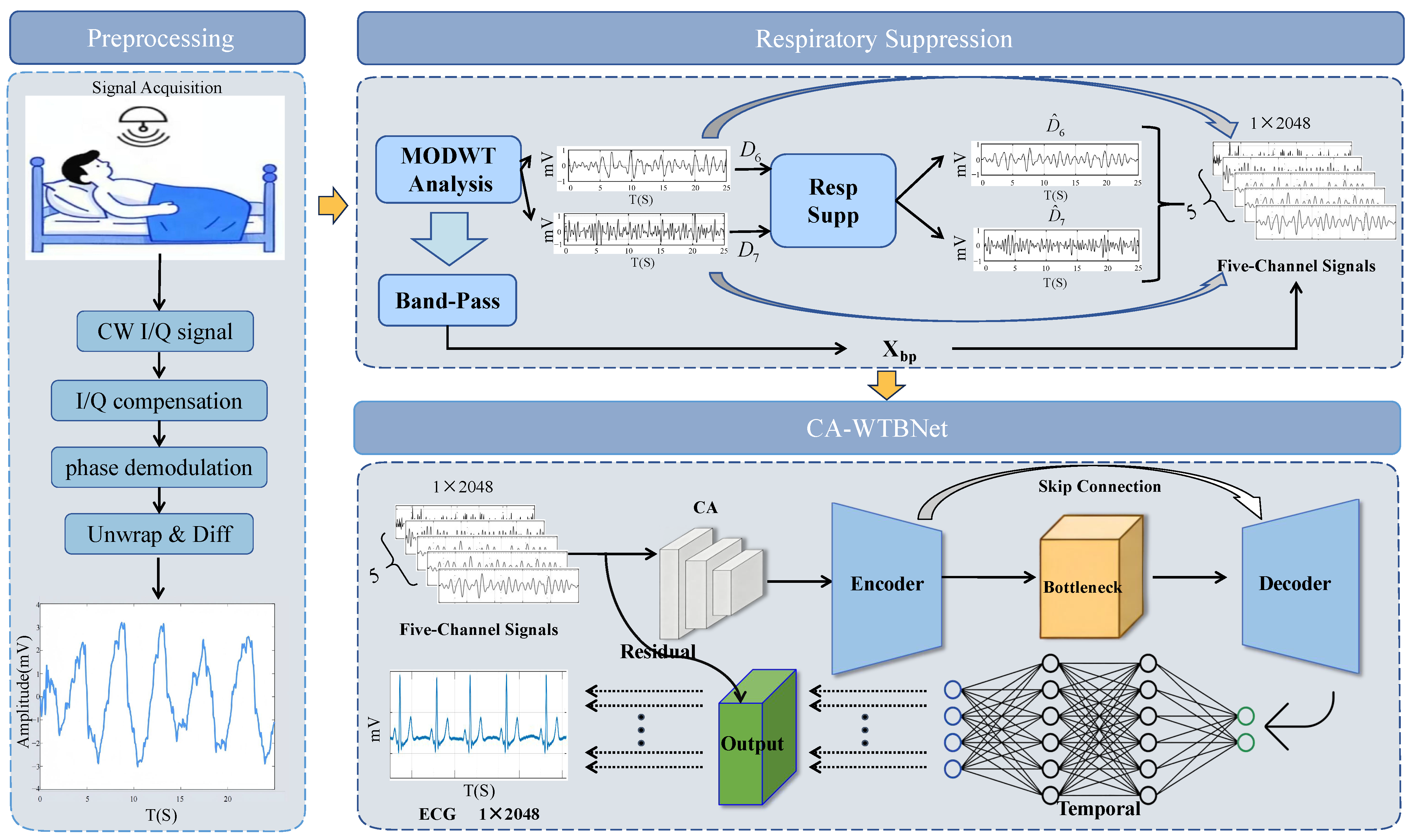
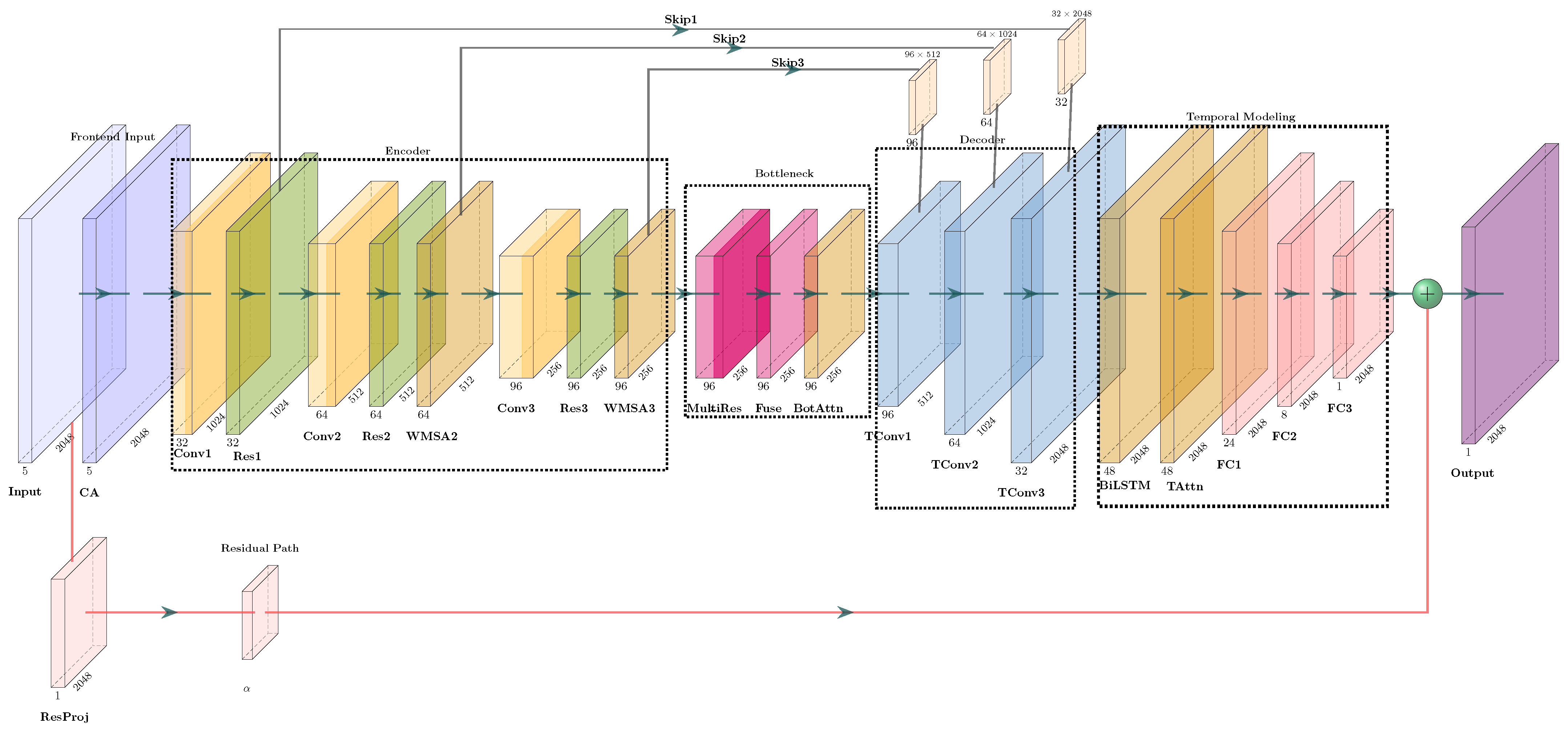
Figure 4. The network is termed CA-WTBNet, which stands for Channel-Attentive Windowed Transformer-BiLSTM Network. It consists of an input channel attention module, a convolutional encoder with window-based Transformer blocks, a bottleneck feature enhancement module, a decoder with skip connections, and a temporal modeling and output reconstruction module based on BiLSTM.
4.3.1. Channel Attention Module
After the multi-channel frontend representation is constructed, heartbeat-related information is not uniformly distributed across different input channels. Therefore, an equal-weight fusion strategy may be insufficient to distinguish the relative importance of different components. To address this issue, a channel attention (CA) module is designed based on the Squeeze-and-Excitation Network (SENet) mechanism [
33], which adaptively assigns different weights to different input channels. The structure of the CA module is illustrated in
Figure 5. This module enhances channels containing more informative heartbeat-related components, while further suppressing redundant channels affected by residual respiration, motion artifacts, and noise. Let the raw frontend input be denoted as
, where
B is the batch size,
is the number of input channels, and
L is the temporal length. In this study,
, corresponding to
,
,
,
, and
. The channel attention weights are generated by Equation (
9).
where
denotes global average pooling along the temporal dimension,
and
are learnable weight matrices,
and
are bias terms, and
is the sigmoid function. The recalibrated input to the encoder is then obtained using Equation (
10).
where ⊙ denotes channel-wise multiplication with broadcasting along the temporal dimension. The resulting
is used as the encoder input, allowing the network to emphasize informative ECG-related channels while suppressing redundant or noise-dominated components.
4.3.2. Encoder Module
The encoder is designed to extract hierarchical temporal representations from the multi-channel mmWave radar features. Let the output of the input channel attention module be denoted as
, where
B is the batch size,
is the number of input channels, and
L is the temporal length. As shown in
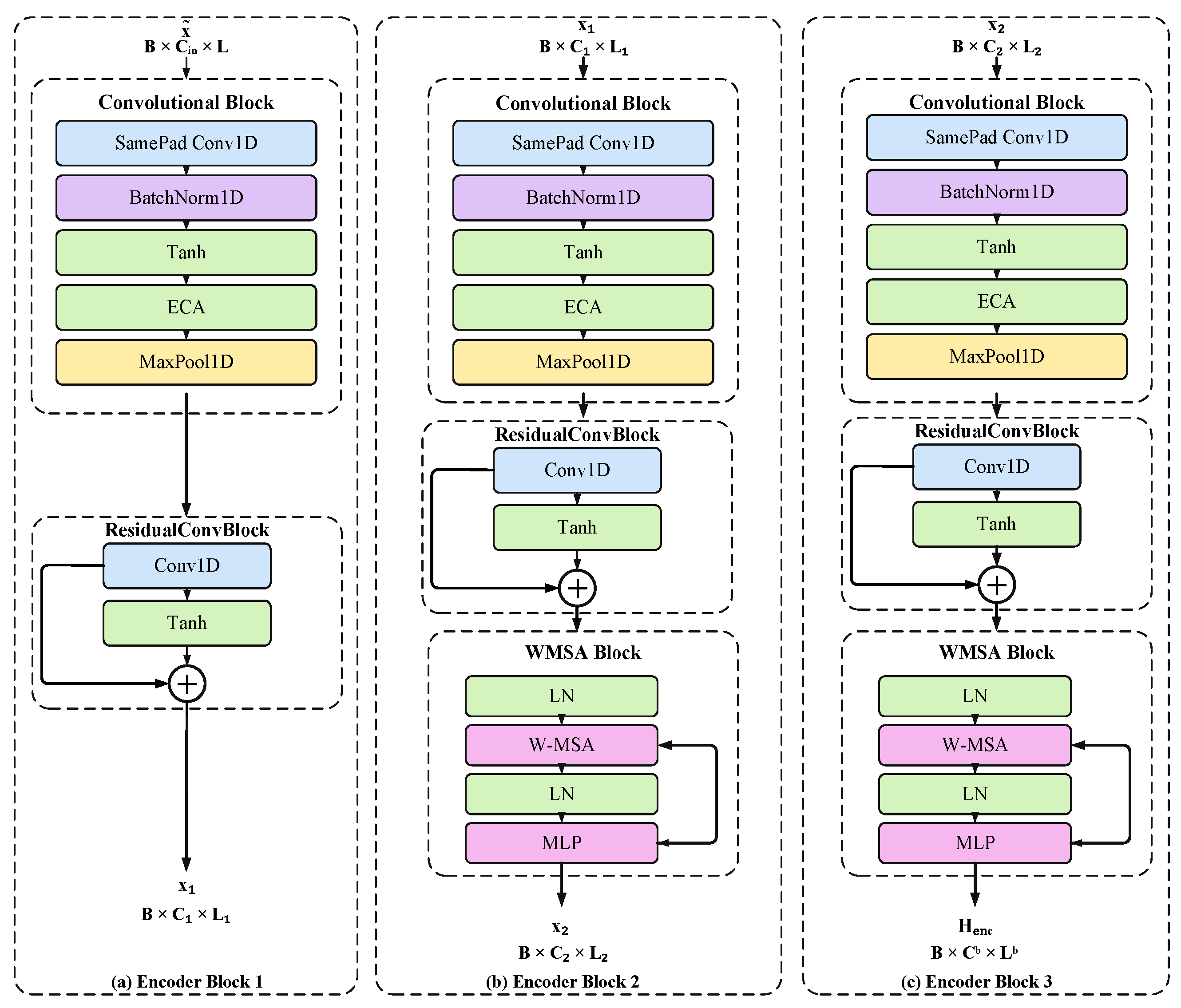
Figure 6, the encoder consists of three convolutional encoding stages. Each stage contains a convolutional block and a residual convolutional block, while window-based Transformer blocks are inserted after the second and third stages to strengthen temporal dependency modeling.
Set
. The encoder gradually transforms the input representation through three hierarchical stages as described in Equation (
11)–(
13). The first stage mainly extracts local waveform features and the second and third stages further introduce window-based Transformer blocks to enhance the temporal dependency modeling:
Here,
and
denote the intermediate encoder features, while
denotes the final encoder representation.
,
, and
represent the channel numbers at different encoding stages, and
,
, and
denote the corresponding temporal lengths.
Each convolutional block is used to perform local waveform feature extraction and downsampling. Specifically, a same-padded one-dimensional convolution [
34] is followed by batch normalization [
35], tanh activation, Efficient Channel Attention (ECA)-based channel recalibration, and max-pooling. For an input feature
, the ECA operation is defined as Equation (
14).
where
denotes global average pooling along the temporal dimension,
denotes a lightweight one-dimensional convolution with kernel size
k for modeling local cross-channel interactions,
is the sigmoid function, and ⊙ denotes channel-wise multiplication. Following ECA-Net [
36], the kernel size
k is adaptively determined by the channel number
C as Equation (
15).
where
denotes the nearest odd integer, and
and
b are set to 2 and 1, respectively. Through this operation, the convolutional block can adaptively emphasize informative feature channels and suppress redundant responses.
The residual convolutional block is further introduced after each convolutional block to refine the extracted temporal features. It uses residual learning to preserve the input information while enhancing local morphological patterns. This design helps to stabilize feature propagation and improves the representation of weak heartbeat-related components in non-stationary radar signals.
To enhance the encoder’s ability to capture long-range temporal dependencies, we incorporate a self-attention mechanism. The window-based multi-head self-attention (W-MSA) design is inspired by efficient Transformer architectures such as Swin Transformer [
37]. Rather than applying full-sequence global attention, which can be computationally heavy, the W-MSA operates within local windows. This approach allows the model to efficiently capture temporal relationships inside each window while keeping the computational cost manageable. Accordingly, W-MSA is applied to the intermediate and high-level encoder features. For an input feature
, the attention sublayer is formulated as Equation (
16).
Here,
is a learnable residual scaling factor and
denotes window-based multi-head self-attention. Specifically, within each local temporal window, the W-MSA operation is computed as Equation (
17).
where
,
and
refer to the query, key, and value matrices in a local window, respectively;
is the dimension of the key vectors; and
is the attention mask used to confine the attention computation within the corresponding window. This enables the model to attend to temporal relationships without the high computational cost of self-attention over the entire sequence.
The feed-forward network (FFN) sublayer is then given by Equation (
18).
where
is another learnable residual scaling factor. Here,
denotes the feed-forward network and
denotes layer normalization.
The encoder progressively reduces the temporal resolution via successive convolution, residual refinement, and window-based self-attention, and enhances the feature representation capacity. The convolutional blocks are designed to learn the local patterns of the heartbeat. The residual convolutional blocks improve the learned features. Furthermore, the window-based Transformer blocks are used to learn the long-range dependencies more effectively. Overall, the encoder produces an efficient and ECG-informative representation for the subsequent bottleneck feature enhancement module.
4.3.3. Bottleneck Feature Enhancement Module
After the encoder, a bottleneck feature enhancement module is introduced to further refine the compressed high-level representation before temporal resolution recovery. Let the encoder output be denoted as , where B is the batch size, is the number of bottleneck feature channels, and is the reduced temporal length. At this stage, the temporal resolution has been reduced, while the channel dimension has been increased. Therefore, the bottleneck module is designed to enhance the compact feature representation by combining multi-scale convolutional feature extraction and attention-based dependency modeling.
First, a multi-resolution convolutional branch is applied to
. This branch contains several parallel one-dimensional convolutional paths with different kernel sizes. These parallel paths allow the network to capture temporal patterns over different receptive-field scales. In this study, the kernel set is denoted as
. The multi-resolution feature extraction process is formulated as Equation (
19).
where
denotes a one-dimensional convolutional branch with kernel size
k,
denotes the channel-wise concatenation of features extracted by all branches, and
denotes a
convolution used for feature fusion. Through the parallel convolutional branches, the module can simultaneously capture short-term local morphological variations and broader temporal patterns in the compressed feature space.
The multi-resolution feature is then added back to the original encoder output through a residual connection. This residual fusion preserves the original high-level representation while introducing multi-scale temporal information. As described in Equation (
20), the fused feature is further processed by a bottleneck attention module to obtain the bottleneck representation:
Here,
denotes the enhanced bottleneck representation and
denotes the attention operation applied in the bottleneck feature space. Since this attention module operates on the compressed temporal representation, it can model long-range dependencies with a moderate computational cost.
Through this design, the bottleneck module further strengthens the encoder output prior to temporal resolution recovery. The multi-resolution branch enriches the feature representation at different temporal scales, whereas the bottleneck attention module improves the modeling of global temporal dependencies. The enhanced representation is then passed to the decoder for temporal resolution recovery.
4.3.4. Decoder Module
The decoder is used to gradually recover the temporal resolution from the compressed bottleneck representation and generate features for ECG waveform reconstruction. Let the bottleneck output be denoted as , where B is the batch size, is the number of bottleneck feature channels, and is the reduced temporal length. The decoder consists of three transposed-convolution stages, which progressively upsample the feature map along the temporal dimension.
To preserve multi-level temporal information learned by the encoder, skip connections are introduced between the encoder and decoder. Specifically, the final encoder output and two intermediate encoder features are reused during decoding. Let
,
, and
, where
,
, and
represent the deep, intermediate, and shallow encoder features, respectively. For each decoding stage, the corresponding skip feature is first temporally aligned by linear interpolation and then projected by a
convolution to match the channel dimension of the decoder feature. The decoding process is formulated as Equations (
21)–(
23).
Here,
denotes the
i-th transposed-convolution block,
denotes linear interpolation used for temporal alignment, and
denotes the
convolution used for channel matching before skip fusion. The coefficient
is a learnable skip-scaling factor that controls the contribution of the corresponding encoder feature. The three skip paths correspond to Skip Conv3, Skip Conv2, and Skip Conv1 respectively.
Through progressive transposed convolution and multi-level skip fusion, the decoder restores the temporal resolution while retaining encoder features at different temporal scales. The deep skip feature provides compact high-level information, whereas the intermediate and shallow skip features help preserve local ECG morphological details. In this way, the decoder provides temporally recovered and morphology-aware features for the subsequent BiLSTM-based reconstruction module.
4.3.5. Temporal Modeling and Output Reconstruction Module
After the decoder, a temporal modeling and output reconstruction module is used to generate the final ECG waveform. Let the decoder output be denoted as , where B is the batch size, is the number of decoder output channels, and L is the temporal length. The feature map is rearranged along the temporal dimension into a sequence matrix , where represents the feature vector at the t-th time step.
The morphology and duration of individual ECG waveform components exhibit bidirectional dependencies. Specifically, in ECG signals, the waveform features at a given time step are associated not only with preceding cardiac electrical activity, but also with subsequent cardiac electrical activity [
38]. LSTM is a recurrent neural network architecture for sequential data processing that includes three gates, namely the input gate, forget gate, and output gate, along with a cell state [
39]. BiLSTM is a bidirectional extension of LSTM [
40]. Therefore, we begin by using BiLSTM to model temporal dependencies in the forward
direction and the backward direction
. The bidirectional temporal representation is given by Equation (
24).
By using bidirectional recurrent modeling, the network can exploit temporal context from both past and future time steps, which is beneficial for maintaining the continuity of the reconstructed ECG waveform.
To further emphasize ECG-informative time positions, a temporal attention module shown in Equation (
25) is applied to the BiLSTM output:
where
is the attention weight at the
t-th time step and
and
are learnable parameters. This operation allows the model to assign larger weights to time positions that contain more useful ECG-related information.
The attention-weighted features are then fed into a time-distributed fully connected mapping module to produce an initial ECG reconstruction . This module maps each temporal feature vector to one ECG amplitude value, and the outputs over all time steps form the reconstructed waveform. The mapping module consists of three fully connected layers with nonlinear activation and dropout between adjacent layers.
Finally, an input-to-output residual connection is introduced to preserve low-level temporal information from the original frontend input. The final reconstructed ECG waveform is defined as Equation (
26).
Here,
denotes the final reconstructed ECG signal,
denotes the original multi-channel frontend input,
projects the input feature to a single-channel residual component, and
is a learnable residual scaling factor.
Overall, this module combines BiLSTM-based temporal modeling, temporal attention, fully connected amplitude mapping, and residual output fusion. It enables the network to capture long-range temporal dependencies while preserving useful low-level information, thereby improving the temporal consistency and morphological stability of the reconstructed ECG waveform.
4.3.6. Multi-Objective Loss Function
To improve the quality of ECG reconstruction, this study adopts a multi-objective loss function to jointly optimize amplitude accuracy, waveform correlation, spectral consistency, and multi-scale morphological similarity. The total loss is defined as Equation (
27).
The corresponding weights were empirically set to
,
,
, and
.
The Huber loss is used as the basic point-wise reconstruction loss, which is calculated in Equation (
28):
where
N denotes the number of ECG samples used in the loss calculation,
and
denote the reconstructed and reference ECG samples, respectively, and
.
The PCC loss in Equation (
29) is used to enhance the global waveform correlation between the reconstructed and reference ECG signals:
where
B denotes the batch size,
and
denote the reconstructed and reference ECG segment of the
b-th sample, respectively,
and
are their temporal mean values,
denotes the Euclidean norm, and
is a small constant used for numerical stability.
The frequency-domain loss in Equation (
30) is then introduced using the fast Fourier transform (FFT) to preserve spectral consistency between the reconstructed and reference ECG signals:
Furthermore, a multi-scale PCC loss shown in Equation (
31) is used to constrain waveform similarity at different temporal resolutions:
where
denotes average pooling with kernel size and stride equal to
s. This multi-objective design encourages the model to reconstruct ECG signals with accurate amplitudes, high waveform correlation, consistent spectral characteristics, and stable morphology across multiple temporal scales.