Author Contributions
Conceptualization, B.V., J.H. and A.W.; methodology, B.V.; software, B.V.; validation, B.V.; formal analysis, B.V.; investigation, B.V.; resources, R.A.; data curation, B.V. and R.A.; writing—original draft preparation, B.V.; writing—review and editing, B.V., J.H., A.W. and R.A.; visualization, B.V.; supervision, J.H. and A.W.; project administration, B.V.; funding acquisition, B.V. All authors have read and agreed to the published version of the manuscript.
Appendix A. Dataset Details
This section provides further details regarding the composition of the LUSData and COVIDx-US datasets, stratified by different attributes.
Table A1 provides a breakdown of the characteristics of the unlabelled data, training set, validation set, local test set, and external test set. As can be seen in the table, the external test set’s manufacturer and probe type distributions differ greatly from those in the local test set. As such, the external test set constitutes a meaningful assessment of generalizability for models trained using the LUSData dataset.
Table A2 provides similar information for the COVIDx-US dataset [
27]. Note that the probe types listed in
Table A1 and
Table A2 are predictions produced by a product (UltraMask, Deep Breathe Inc., London, ON, Canada) and not from metadata accompanying the examinations.
Table A1.
Characteristics of the ultrasound videos in the LUSData dataset. The number of videos possessing known values for a variety of attributes are displayed. Percentages of the total in each split are provided as well, but some do not sum to 100 due to rounding.
Table A1.
Characteristics of the ultrasound videos in the LUSData dataset. The number of videos possessing known values for a variety of attributes are displayed. Percentages of the total in each split are provided as well, but some do not sum to 100 due to rounding.
| | Local | External |
|---|
| | Unlabelled | Train | Validation | Test | Test |
|---|
| Probe Type | | | | | |
| Phased Array | 50,769 | | | | |
| Curved Linear | | | | | |
| Linear | | | | | |
| Manufacturer | | | | | |
| Sonosite | 53,663 | | | | |
| Mindray | | | | | |
| Philips | | | | | |
| Esaote | | | | | |
| GE § | | | | | |
| Depth (cm) | | | | | |
| Mean [STD] | | | | | |
| Unknown | | | | | |
| Environment | | | | | |
| ICU † | 43,839 | | | | |
| ER ‡ | 13,280 | | | | |
| Ward | | | | | |
| Urgent Care | | | | | |
| Unknown | | | | | |
| Patient Sex | | | | | |
| Male | 30,300 | | | | |
| Female | 20,809 | | | | |
| Unknown | | | | | |
| Patient Age | | | | | |
| Mean [STD] | | | | | - |
| Unknown | | | | | |
| Total | 59,309 | 5679 | 1184 | 1249 | 925 |
Table A2.
Characteristics of the ultrasound videos in the COVIDx-US dataset. The number of videos possessing known values for a variety of attributes is displayed. Percentages of the total in each split are provided as well, but some do not sum to 100 due to rounding.
Table A2.
Characteristics of the ultrasound videos in the COVIDx-US dataset. The number of videos possessing known values for a variety of attributes is displayed. Percentages of the total in each split are provided as well, but some do not sum to 100 due to rounding.
| | Train | Validation | Test |
|---|
| Probe Type | | | |
| Phased Array | | | |
| Curved Linear | | | |
| Linear | | | |
| Patient Sex | | | |
| Male | | | |
| Female | | | |
| Unknown | | | |
| Patient Age | | | |
| Mean [STD] | | | |
| Unknown | | | |
| Total | 169 | 42 | 31 |
Appendix B. Transformation Runtime Estimates
We aimed to examine relative runtime differences between the transformations used in this study. Runtime estimates were obtained for each transformation in the StandardAug and AugUS-v1 pipelines. Estimates were calculated by conducting the transformation 1000 times using the same image. The experiments were run on a system with an Intel i9-10900K CPU at GHz. Python 3.11 was utilized, and the transforms were written using PyTorch version 2.2.1 and TorchVision 0.17.1. Note that runtime may vary considerably depending on the software environment and underlying hardware.
Appendix C. StandardAug Transformations
We investigated a standard data augmentation pipeline that has been used extensively in the SSL literature [
14,
15,
16,
17]. To standardize experiments, we adopted the symmetric version from the VICReg paper [
17], which uses the same transformations and probabilities for each of the two branches in the joint embedding architecture. The transformations and their parameter settings are widely adopted. Below, we detail their operation and parameter assignments.
Appendix C.1. Crop and Resize (A00)
A rectangular crop of the input image is designated at a random location. The area of the cropped region is sampled from the uniform distribution . The cropped region’s aspect ratio is sampled from the uniform distribution . Its width and height are calculated accordingly. The cropped region is then resized to the original image dimension.
Appendix C.2. Horizontal Reflection (A01)
The image is reflected about the central vertical axis.
Appendix C.3. Colour Jitter (A02)
The brightness, contrast, saturation, and hue of the image are modified. The brightness change factor, contrast change factor, saturation change factor, and hue change factor are sampled from , , , and , respectively.
Appendix C.4. Conversion to Grayscale (A03)
Images are converted to grayscale. The output images have three channels, such that each channel has the same pixel intensity.
Appendix C.5. Gaussian Blur (A04)
The image is denoised using a Gaussian blur with kernel size 13 and standard deviation sampled uniformly at random from . Note that in the original pipeline, the kernel size was set to 23 and images were used. We used images; as such, we selected a kernel size that covers a similar fraction of the image.
Appendix C.6. Solarization (A05)
All pixels with an intensity of 128 or greater are inverted. Note that the inputs are unsigned 8-bit images.
Appendix D. Ultrasound-Specific Transformations
In this section, we provide details on the set of transformations that comprise AugUS-v1.
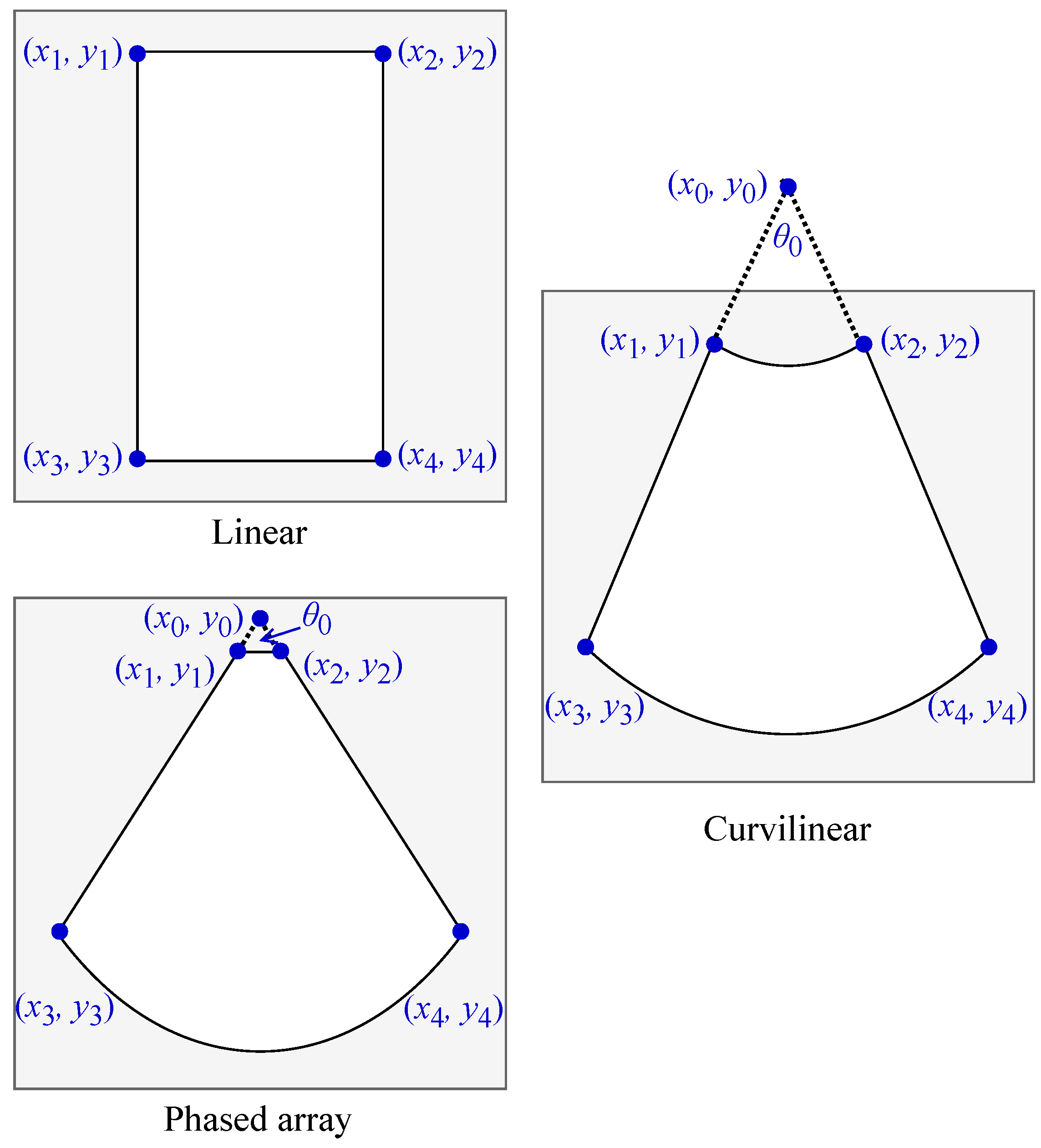
Several of the transformations operate on the pixels contained within the ultrasound field of view (FOV). As such, the geometrical form of the FOV was required to perform some transformations. We adopted the same naming convention for the vertices of the ultrasound FOV as Kim et al. [
44]. Let
,
,
, and
represent the respective locations of the top left, top right, bottom left, and bottom right vertices, and let
be the x- and y-coordinates of
in image space. For convex FOV shapes, we denote the intersection of lines
and
as
.
Figure A1 depicts the arrangement of these points for each of the three main ultrasound FOV shapes: linear, curvilinear, and phased array. A software tool was used to estimate the FOV shape and probe type for all videos in each dataset (UltraMask, Deep Breathe Inc., Canada).
Figure A1.
Locations of the named FOV vertices for each of the three main field of view shapes in ultrasound imaging.
Figure A1.
Locations of the named FOV vertices for each of the three main field of view shapes in ultrasound imaging.
Appendix D.1. Probe Type Change (B00)
To produce a transformed ultrasound image with a different FOV shape, a mapping that gives the location of pixels in the original image for each coordinate in the new image is calculated. Concretely, the function returns the coordinates of the point in the original image that corresponds to a point in the transformed image. Note that corresponds to the top left of the original image. Pixel intensities in the transformed image are interpolated according to their corresponding location in the original image.
Algorithm A1 details the calculation of for converting linear FOVs to convex FOVs with a random radius factor , along with new FOV vertices. Similarly, curvilinear and phased array FOV shapes are converted to linear FOV shapes. Algorithm A2 details the calculation of the mapping that transforms convex FOV shapes to linear shapes, along with calculations for the updated named coordinates. To ensure that no aspects of the old FOV remain on the image, bitmask is produced using the new named coordinates.
Since the private dataset was resized to square images that exactly encapsulated the FOV, images were resized to match their original aspect ratios to ensure that the sectors were circular. They are then resized to their original dimensions following the transformation.
| Algorithm A1 Compute a point mapping for linear to curvilinear FOV shape, along with new FOV vertices |
- Require:
FOV vertices , , , ; radius factor ; coordinate maps and
|
- 1:
| ▹Bottom sector radius |
- 2:
|
- 3:
| ▹Lateral bounds will intersect at |
- 4:
- 5:
- 6:
- 7:
|
- 8:
| ▹Top sector radius |
- 9:
| ▹Angle with the central vertical |
- 10:
| ▹Final coordinate mapping |
- 11:
return , , , ,
| ▹Coordinate mapping, new FOV vertices |
| Algorithm A2 Compute a point mapping for convex to linear FOV shape, along with new FOV vertices |
- Require:
FOV vertices , , , ; point of intersection ; angle of intersection ; width fraction ; coordinate maps and
|
- 1:
| ▹Bottom sector radius |
- 2:
- 3:
- 4:
- 5:
|
- 6:
| ▹Angle with the central vertical |
- 7:
| ▹Normalized y-coordinates |
- 8:
if probe type is curvilinear then
|
- 9:
| ▹ Curvilinear; top sector radius |
- 10:
else
|
- 11:
| ▹ Phased array; distance to top bound |
- 12:
end if - 13:
|
- 14:
return , , , ,
| ▹Coordinate mapping, new FOV vertices |
Appendix D.2. Convexity Change (B01)
To mimic an alternative convex FOV shape with a different
, a mapping is calculated that results in a new FOV shape wherein
is translated vertically. A new value for the width of the top of the FOV is randomly calculated, facilitating the specification of a new
. Given the new
, a pixel map
is computed according to Algorithm A3. Similar to the probe type change transformation, pixel intensities at each coordinate in the transformed image are interpolated according to the corresponding coordinate in the original image returned by
.
| Algorithm A3 Compute a point mapping from an original to a modified convex FOV shape. |
- Require:
FOV vertices , , , ; point of intersection ; angle of intersection ; new top width ; coordinate maps and
|
- 1:
| ▹Scale change for top bound |
- 2:
- 3:
- 4:
- 5:
- 6:
angle, point of intersection of and
|
- 7:
| ▹Current bottom radius |
- 8:
| ▹New bottom radius |
- 9:
| ▹Current top radius |
- 10:
| ▹New top radius |
- 11:
- 12:
- 13:
- 14:
|
- 15:
return , , , ,
| ▹Coordinate mapping, new FOV vertices |
Appendix D.3. Wavelet Denoising (B02)
Following the soft thresholding method by Birgé and Massart [
29], we apply a wavelet transform, conduct thresholding, then apply the inverse wavelet transform. The mother wavelet is randomly chosen from a set, and the sparsity parameter
is sampled from a uniform distribution. We use
levels of wavelet decomposition and set the decomposition level
. We designated Daubechies wavelets
as the set of mother wavelets, which is a subset of those identified by Vilimek et al.’s assessment [
31] as most suitable for denoising ultrasound images.
Appendix D.4. Contrast-Limited Adaptive Histogram Equalization (B03)
Contrast-limited adaptive histogram equalization is applied to the input image. The transformation enhances low-contrast regions of ultrasound images while avoiding excessive noise amplification. We found that CLAHE enhances the artifact. The tiles are regions of pixels. The clip limit is sampled from the uniform distribution .
Appendix D.5. Gamma Correction (B04)
The pixel intensities of the image are nonlinearly modified. Pixel intensity
I is transformed as follows:
where
. The gain is fixed at 1.
Appendix D.6. Brightness and Contrast Change (B05)
The brightness and contrast of the image are modified. The brightness change factor, contrast change factor are sampled from , , respectively. The image is then multiplied element-wise by its FOV mask to ensure black regions external to the FOV remain black.
Appendix D.7. Depth Change Simulation (B06)
The image is zoomed about a point that differs according to FOV type, simulating a change in imaging depth. The transformation preserves the centre for linear FOV shapes and preserves for convex FOV shapes. The magnitude of the zoom transformation, d, is randomly sampled from a uniform distribution. Increasing the depth corresponds to zooming out (), while decreasing the depth corresponds to zooming in ().
Appendix D.8. Speckle Noise Simulation (B07)
Following Singh et al.’s method [
32], this transformation calculates synthetic speckle noise and applies it to the ultrasound beam. Various parameters of the algorithm are randomly sampled upon each invocation. The lateral and axial resolutions for interpolation are random integers drawn from the ranges
and
, respectively. The number of synthetic phasors is randomly drawn from the integer range
. Sample points on the image are evenly spaced in Cartesian coordinates for linear beam shapes. For convex beams, the sample points are evenly spaced in polar coordinates.
Appendix D.9. Gaussian Noise Simulation (B08)
Multiplicative Gaussian noise is applied to the pixel intensities across the image. First, the standard deviation of the Gaussian noise, , is randomly drawn from the uniform distribution . Multiplicative Gaussian noise with mean 1 and standard deviation is then applied independently to each pixel in the image.
Appendix D.10. Salt and Pepper Noise Simulation (B09)
A random assortment of points in the image are set to 255 (salt) or 0 (pepper). The fractions of pixels set to salt and pepper values are sampled randomly according to .
Appendix D.11. Horizontal Reflection (B10)
The image is reflected about the central vertical axis. This transformation is identical to A01.
Appendix D.12. Rotation and Shift (B11)
A non-scaling affine transformation is applied to the image. More specifically, the image is translated and rotated. The horizontal component of the translation is sampled from , as a fraction of the image’s width. Similarly, the vertical component is sampled from , as a fraction of the image’s height. The rotation angle, in degrees, is sampled from .
Appendix E. Pleural Line Object Detection Training
The Single Shot Detector (SSD) method [
37] was employed to perform a cursory evaluation of the pretrained models on an object detection task. The
PL task involved localizing instances of the pleural line in LU images, which can be described as a bright horizontal line that is typically situated slightly below the vertical level of the ribs. It is only visible between the rib spaces, since bone blocks the ultrasound scan lines. The artifact represents the interface between the parietal and visceral linings of the lung in a properly acquired LU view.
As in the classification experiments, we used the MobileNetV3Small architecture as the backbone of the network. There is precedent for using the SSD object detection method, as it has been applied to assess the object detection capabilities of MobileNet architectures [
33,
45]. The feature maps outputted from a designated set of layers were passed to the SSD regression and classification heads. We selected a range of layers whose feature maps had varying spatial resolution.
Table A3 provides the identities and dimensions of the feature maps from the backbone that were fed to the SSD model head. The head contained 43,796 trainable parameters, which was light compared to the backbone (927,008).
The set of default anchor box aspect ratios was manually specified after examining the distribution of bounding box aspect ratios in the training set. The 25th percentile was , and the 75th percentile was . The pleural line typically has a much greater width than height. Accordingly, we designated the set of default anchor box aspect ratios () as . Six anchor box scales were used. The first five were spaced out evenly over the range , which corresponds to the square roots of the minimum and maximum areas of the bounding box labels present in the training set, in normalized image coordinates. The final scale is , which is included by default. The box confidence threshold was , and the intersection over union threshold to match anchors to box labels was . The non-maximum suppression (NMS) threshold was , and the number of detected boxes to keep after NMS was 50.
The backbone and head were assigned initial learning rates of
and
, respectively. Learning rates were annealed according to a cosine decay schedule. The model was trained for 30 epochs to minimize the loss function from the original SSD paper, which has a regression component for bounding box offsets and a classification component for distinguishing objects and background [
37]. The weights corresponding to the epoch with the lowest validation loss were retained for test set evaluation.
Table A3.
MobileNetV3Small block indices and the corresponding dimensions of the feature maps that they output, given an input of size .
Table A3.
MobileNetV3Small block indices and the corresponding dimensions of the feature maps that they output, given an input of size .
| Block Index | Feature Map Dimensions () |
|---|
| 1 | |
| 3 | |
| 6 | |
| 9 | |
| 12 | |
Appendix F. Leave-One-Out Analysis Statistical Testing
As outlined in
Section 4.1, statistical testing was performed to detect differences between pretrained models trained using an ablated version of the StandardAug and AugUS-O pipelines and baseline models pretrained on the original pipelines. Each ablated version of the pipeline was missing one transformation from the data augmentation pipeline. Ten-fold cross-validation conducted on the training set provided 10 samples of test AUC metrics for both the A-line versus B-line (
AB) and pleural effusion (
PE) binary classification tasks. The samples were taken as a proxy for test-time performance for linear classifiers trained on each of the above downstream tasks.
To determine whether the mean test AUC for each ablated model was different from the baseline model, hypothesis testing was conducted. The model pretrained using the original pipeline was the control group, while the models pretrained using ablated versions of the pipeline were the experimental groups. First, Friedman’s test [
38] was conducted to determine if there was any difference in the mean test AUC among the baseline and ablated models. We selected a nonparametric multiple comparisons test because of the lack of assumptions regarding normality or homogeneity of variances. Each collection had 10 samples.
Table A4 details the results of Friedman’s test for each pipeline and classification task. Friedman’s test detected differences among the collection of test AUC for both classification tasks with the StandardAug pipeline. Only the
AB task exhibited significant differences for the AugUS-O pipeline.
Table A4.
Friedman test statistics and p-values for mean cross-validation test AUC attained by models pretrained using an entire data augmentation pipeline and ablated versions of it.
Table A4.
Friedman test statistics and p-values for mean cross-validation test AUC attained by models pretrained using an entire data augmentation pipeline and ablated versions of it.
| Pipeline | AB | PE |
|---|
| | Statistic | p-Value | Statistic | p-Value |
|---|
| StandardAug | | * | | * |
| AugUS-O | | * | | |
When the null hypothesis of the Friedman test was rejected, post hoc tests were conducted to determine whether any of the test AUC means in the experimental groups were significantly different than the control group. The Wilcoxon Signed-Rank Test [
39] was designated as the post hoc test, due to its absence of any normality assumptions. Note that for each pipeline,
n comparisons were performed, where
n is the number of transformations within the pipeline. The Holm–Bonferroni correction [
40] was applied to keep the family-wise error rate at
for each pipeline/task combination. Results of the post hoc tests are given in
Table A5. No post hoc tests were performed for the AugUS-O pipeline evaluated on the
PE task because the Friedman test revealed no significant differences.
Table A5.
Test statistics (
T) and
p-values obtained from the Wilcoxon Signed-Rank post hoc tests that compared linear classifiers trained with ablated models’ features to a control linear classifier trained on the baseline model. Experimental groups are identified according to the left-out transformation, as defined in
Table 2 and
Table 3.
| Pipeline | Comparison | AB | PE |
|---|
| | | | p-Value | | p-Value |
|---|
| StandardAug | A00 | 0 | * | 0 | * |
| A01 | 6 | | 21 | |
| A02 | 1 | * | 3 | * |
| A03 | 19 | | 10 | |
| A04 | 9 | | 5 | |
| A05 | 15 | | 10 | |
| AugUS-O | B00 | 18 | | - | - |
| B01 | 8 | | - | - |
| B02 | 0 | * | - | - |
| B03 | 0 | * | - | - |
| B04 | 12 | | - | - |
| B05 | 9 | | - | - |
| B06 | 13 | | - | - |
| B07 | 13 | | - | - |
| B08 | 1 | * | - | - |
| B09 | 1 | * | - | - |
| B10 | 23 | | - | - |
| B11 | 0 | * | - | - |
Appendix G. Additional Positive Pair Examples
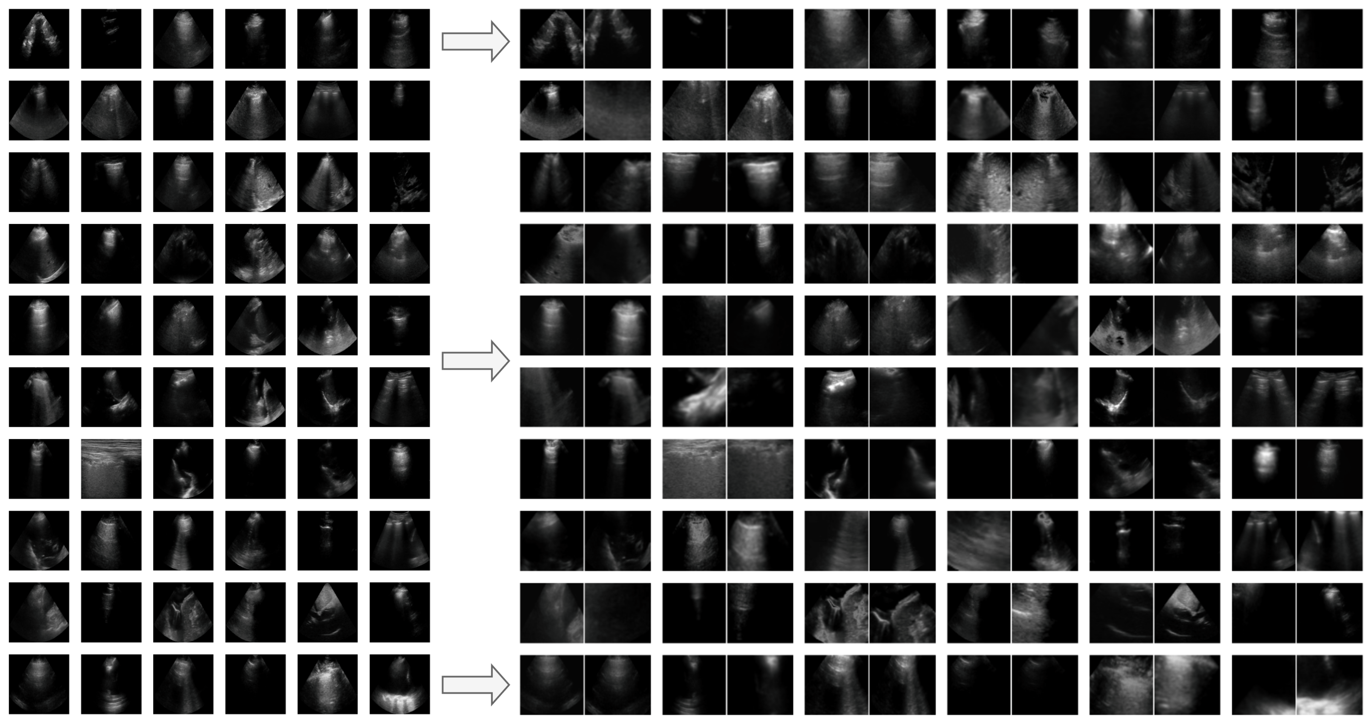
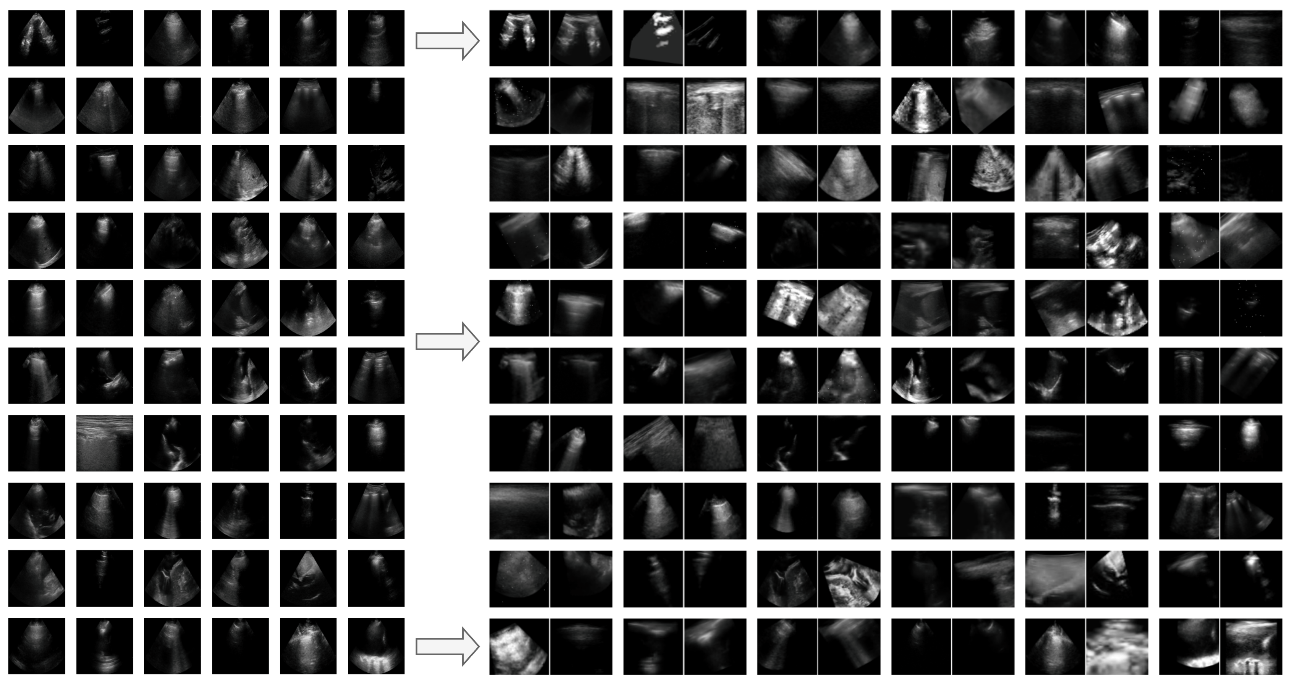
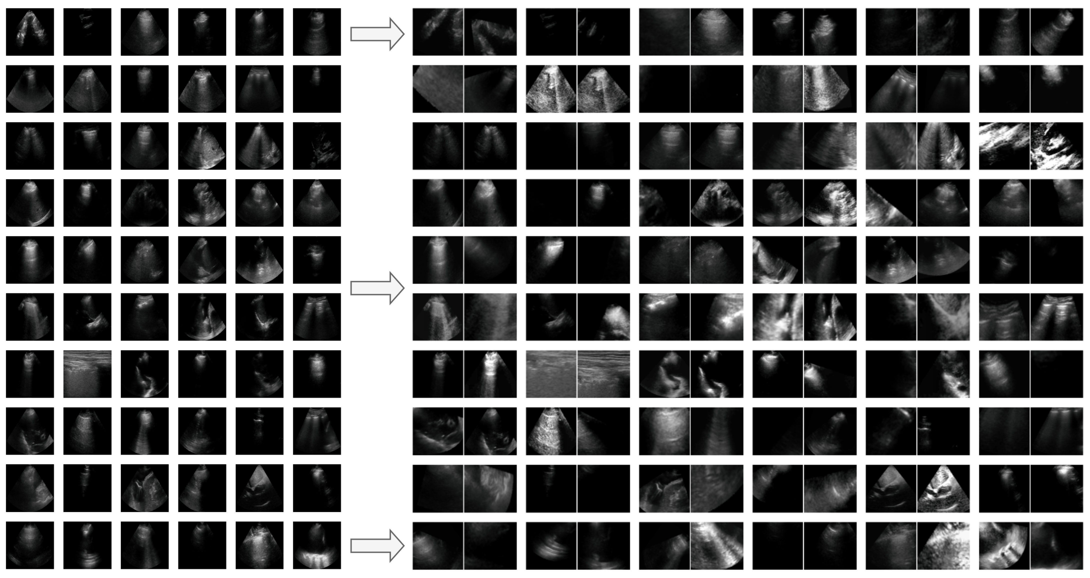
Figure A2,
Figure A3 and
Figure A4 provide several examples of positive pairs produced by the StandardAug, AugUS-O, and AugUS-D pipelines, respectively. Each figure shows original images from LUSData, along with two views of each image that were produced by applying stochastic data augmentation twice to the original images.
Figure A2.
Examples of lung ultrasound images (left) and positive pairs produced using the StandardAug pipeline (right).
Figure A2.
Examples of lung ultrasound images (left) and positive pairs produced using the StandardAug pipeline (right).
Figure A3.
Examples of lung ultrasound images (left) and positive pairs produced using the AugUS-O pipeline (right).
Figure A3.
Examples of lung ultrasound images (left) and positive pairs produced using the AugUS-O pipeline (right).
Figure A4.
Examples of lung ultrasound images (left) and positive pairs produced using the AugUS-D pipeline (right).
Figure A4.
Examples of lung ultrasound images (left) and positive pairs produced using the AugUS-D pipeline (right).
Appendix H. Results with ResNet18 Backbone
As outlined in
Section 3.5, MobileNetV3Small [
33] was selected as the feature extractor for all experiments in this study, primarily due to its suitability for lightweight inference in edge deployment scenarios. It has also been used in prior work for similar tasks [
25,
34]. However, we wanted to determine if similar trends in the results held for an alternate backbone architecture with greater capacity. Larger CNN backbones are frequently used for self-supervised pretraining.
We repeated the experiments in
Section 4.2 and
Section 4.3 using ResNet18 [
42] as the feature extractor, which is a more common architecture. Note that ResNet18’s capacity is far greater than that of MobileNetV3Small—the former has approximately 11,200,000 trainable parameters, while the latter has about 927,000. We applied the same architecture for the projector head that was used for MobileNetV3Small experiments, which was a 2-layer multilayer perceptron with 576 nodes comprising each layer.
ResNet18 feature extractors were pretrained using virtual machines equipped with an Intel Silver 4216 Cascade Lake CPU at GHz and a Nvidia Tesla V100 GPU with 12 GB of VRAM. Supervised learning was conducted using a virtual machine equipped with an Intel E5-2683 v4 Broadwell CPU at GHz and a Nvidia Tesla P100 GPU.
Table A6 displays the performance of pretrained ResNet18 backbones when evaluated on the LUSData test set for the
AB,
PE, and
COVID tasks. Most fine-tuned models exhibited overfitting, likely due to the architecture’s capacity. Notably, the pretrained models tended to exhibit overfitting when fine-tuned, while the fully supervised ImageNet-pretrained model achieved strong performance on
AB and
PE. Linear classifiers trained on frozen pretrained backbones’ output features generally achieved the strongest performance and avoided overfitting. Consistent with MobileNetV3Small, the use of cropping-based augmentation pipelines translated to greater performance on
AB and
PE in the linear evaluation setting. In the fine-tuning setting, the backbone pretrained using AugUS-O exhibited markedly poorer performance on
AB but achieved the greatest test AUC on
PE. On the
COVID test set, the backbone pretrained using the AugUS-O pipeline led to the greatest average AUC in both the linear and fine-tuning settings.
Table A6.
Test set performance for linear classification (LC) and fine-tuning (FT) experiments with the COVID task using pretrained ResNet18 backbones. For COVID, metrics are averages across all four classes. The best observed metrics in each experimental setting are in boldface.
Table A6.
Test set performance for linear classification (LC) and fine-tuning (FT) experiments with the COVID task using pretrained ResNet18 backbones. For COVID, metrics are averages across all four classes. The best observed metrics in each experimental setting are in boldface.
Train
Setting | Task | Weights | Pipeline | Accuracy | Precision | Recall | AUC |
|---|
| LC | AB | SimCLR | StandardAug | | | | |
| SimCLR | AugUS-O | | | | |
| SimCLR | AugUS-D | | | | |
| ImageNet | - | | | | |
| PE | SimCLR | StandardAug | | | | |
| SimCLR | AugUS-O | | | | |
| SimCLR | AugUS-D | | | | |
| ImageNet | - | | | | |
| COVID | SimCLR | StandardAug | | | | |
| SimCLR | AugUS-O | | | | |
| SimCLR | AugUS-D | | | | |
| ImageNet | - | | | | |
| FT | AB | SimCLR | StandardAug | | | | |
| SimCLR | AugUS-O | | | | |
| SimCLR | AugUS-D | | | | |
| Random | - | | | | |
| ImageNet | - | | | | |
| PE | SimCLR | StandardAug | | | | |
| SimCLR | AugUS-O | | | | |
| SimCLR | AugUS-D | | | | |
| Random | - | | | | |
| ImageNet | - | | | | |
| COVID | SimCLR | StandardAug | | | | |
| SimCLR | AugUS-O | | | | |
| SimCLR | AugUS-D | | | | |
| Random | - | | | | |
| ImageNet | - | | | | |
The fine-tuned backbones and linear classifiers were also evaluated on the external test set for the
AB and
PE tasks.
Table A7 displays the performance of pretrained ResNet18 backbones when evaluated on the LUSData test set for the
AB and
PE tasks. Again, linear classifiers with pretrained backbones mostly achieved greater performance than fine-tuned classifiers. Backbones pretrained with the StandardAug pipeline achieved the greatest external test set AUC for the
AB task. However, those pretrained with AugUS-O performed comparably with StandardAug for the
PE task under the linear evaluation setting but achieved the greatest AUC in the fine-tuning setting.
Table A7.
External test set performance for linear classifiers (LCs) and fine-tuned models (FTs). The best observed metrics in each experimental setting are in boldface.
Table A7.
External test set performance for linear classifiers (LCs) and fine-tuned models (FTs). The best observed metrics in each experimental setting are in boldface.
Train
Setting | Task | Initial
Weights | Pipeline | Accuracy | Precision | Recall | AUC |
|---|
| LC | AB | SimCLR | StandardAug | | | | |
| SimCLR | AugUS-O | | | | |
| SimCLR | AugUS-D | | | | |
| ImageNet | - | | | | |
| PE | SimCLR | StandardAug | | | | |
| SimCLR | AugUS-O | | | | |
| SimCLR | AugUS-D | | | | |
| ImageNet | - | | | | |
| FT | AB | SimCLR | StandardAug | | | | |
| SimCLR | AugUS-O | | | | |
| SimCLR | AugUS-D | | | | |
| Random | - | | | | |
| ImageNet | - | | | | |
| PE | SimCLR | StandardAug | | | | |
| SimCLR | AugUS-O | | | | |
| SimCLR | AugUS-D | | | | |
| Random | - | | | | |
| ImageNet | - | | | | |
Two key observations were drawn from these experiments. First, the low-capacity MobileNetV3Small backbones achieved similar performance to the high-capacity ResNet18 backbones for these LU tasks when their weights were frozen (i.e., linear classifiers). Second, with a higher-capacity backbone, linear classifiers trained on the features outputted by SSL-pretrained backbones often achieved greater performance than fine-tuning despite the weight initialization strategy. The opposite trend was observed for backbones initialized with ImageNet-pretrained weights.
Appendix I. Label Efficiency Statistical Testing
For each of the AB and PE tasks, there were five experimental conditions: SimCLR pretraining with the StandardAug pipeline, SimCLR pretraining with the AugUS-O pipeline, SimCLR pretraining with the AugUS-D pipeline, ImageNet weight initializations, and random weight initialization. The population consisted of 20 subsets of the training set that were split randomly by patient. The same splits were used across all conditions, reflecting a repeated measures design. The experiment was repeated separately for the AB and the PE task.
The Friedman Test Statistic (
) was
for
AB, with a
p-value of 0. For
PE, the
, and the
p-value was 0. As such, the null hypothesis was rejected for both cases, indicating the existence of differences in the mean test AUC across conditions. The Wilcoxon Signed-Rank Test was performed as a post hoc test between each pair of populations.
Table A8 and
Table A9 provide all Wilcoxon Test Statistics, along with
p-values and differences in the medians between conditions. The Bonferroni correction was applied to the
p-values to keep the family-wise error rate to
. Statistically significant comparisons are indicated.
Table A8.
Test statistics (T) and p-values obtained from the Wilcoxon Signed-Rank post hoc tests comparing LUSData test AUC on AB for classifiers trained on subsets of the training set. For comparison , . The displayed p-values have been adjusted according to the Bonferroni correction to control the family-wise error rate.
| Comparison | T | p-Value | |
|---|
| Random/ImageNet | 3 | 9.4 × 10⁻⁵ * | |
| Random/StandardAug | 0 | 1.9 × 10⁻⁵ * | |
| Random/AugUS-O | 12 | 1.3 × 10⁻³ * | |
| Random/AugUS-D | 0 | 1.9 × 10⁻⁵ * | |
| ImageNet/StandardAug | 0 | 1.9 × 10⁻⁵ * | |
| ImageNet/AugUS-O | 0 | 1.9 × 10⁻⁵ * | |
| ImageNet/AugUS-D | 0 | 1.9 × 10⁻⁵ * | |
| StandardAug/AugUS-O | 0 | 1.9 × 10⁻⁵ * | |
| StandardAug/AugUS-D | 61 | 1.0 | |
| AugUS-O/AugUS-D | 0 | 1.9 × 10⁻⁵ * | |
Table A9.
Test statistics (T) and p-values obtained from the Wilcoxon Signed-Rank post hoc tests comparing LUSData test AUC on PE for classifiers trained on subsets of the training set. For comparison , . The displayed p-values have been adjusted according to the Bonferroni correction to control the family-wise error rate.
| Comparison | T | p-Value | |
|---|
| Random/ImageNet | 1 | 3.8 × 10⁻⁵ * | |
| Random/StandardAug | 31 | 4.2 × 10⁻² * | |
| Random/AugUS-O | 16 | 3.2 × 10⁻³ * | |
| Random/AugUS-D | 5 | 1.9 × 10⁻⁴ * | |
| ImageNet/StandardAug | 1 | 3.8 × 10⁻⁵ * | |
| ImageNet/AugUS-O | 0 | 1.9 × 10⁻⁵ * | |
| ImageNet/AugUS-D | 1 | 3.8 × 10⁻⁵ * | |
| StandardAug/AugUS-O | 57 | 7.6 × 10⁻¹ | |
| StandardAug/AugUS-D | 53 | 5.3 × 10⁻¹ | |
| AugUS-O/AugUS-D | 78 | 1 | |
Appendix J. Additional Random Crop and Resize Experiments
The C&R transform encourages pretrained representations to be invariant to scale. It is also believed that the C&R transform instills invariance between global and local views or between disjoint views of the same object type [
14]. While the minimum area of the crop determines the magnitude of the scaling transformations, the aspect ratio range dictates the difference in distortion in both axes of the image. The default aspect ratio range is
. We pretrained with the AugUS-D pipeline using a fixed aspect range of 1 and
, which resulted in a test AUC of
for
AB and
for
PE in the LC training setting. Compared to the regular AugUS-D that uses the default aspect ratio range (
Table 5),
AB test AUC remained unchanged, and
PE test AUC decreased by
.
Lastly, we conducted pretraining on LUSData using only the C&R transformation; that is, the data augmentation pipeline was [A00]. Recent work by Moutakanni et al. [
46] suggests that, with sufficient quantities of training data, competitive performance in downstream computer vision tasks can be achieved using crop and resize as the sole transformation in joint embedding SSL. Linear evaluation of a feature extractor pretrained with only C&R yielded test AUC of
and
on
AB and
PE, respectively. Compared to the linear evaluations presented in
Section 4, these metrics are greater than those achieved using AugUS-O, but less than those achieved with StandardAug or AugUS-D. It is evident that C&R is a powerful transformation for detecting local objects.
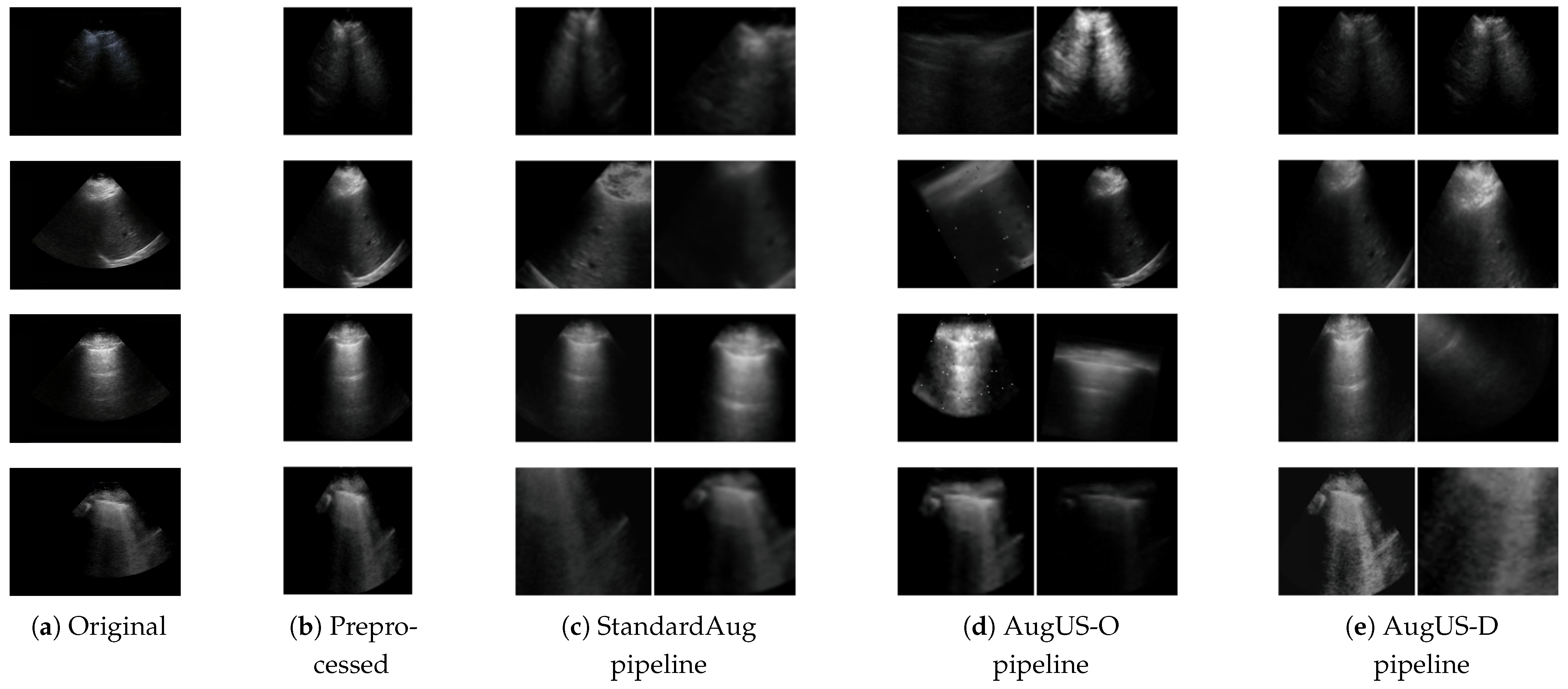
Figure 1.
Examples of the preprocessing and data augmentation methods in this study. (a) Original images are from ultrasound exams. (b) Semantics-preserving preprocessing is applied to crop out areas external to the field of view. (c) The StandardAug pipeline is a commonly employed data augmentation pipeline in self-supervised learning. (d) The AugUS-O pipeline was designed to preserve semantic content in ultrasound images. (e) AugUS-D is a hybrid pipeline whose construction was informed by empirical investigations into the StandardAug and AugUS-O pipelines.
Figure 2.
Raw ultrasound images are preprocessed by performing an element-wise multiplication (⊗) of the raw image with a binary mask that preserves only the field of view, then cropped according to the bounds of the field of view.
Figure 2.
Raw ultrasound images are preprocessed by performing an element-wise multiplication (⊗) of the raw image with a binary mask that preserves only the field of view, then cropped according to the bounds of the field of view.
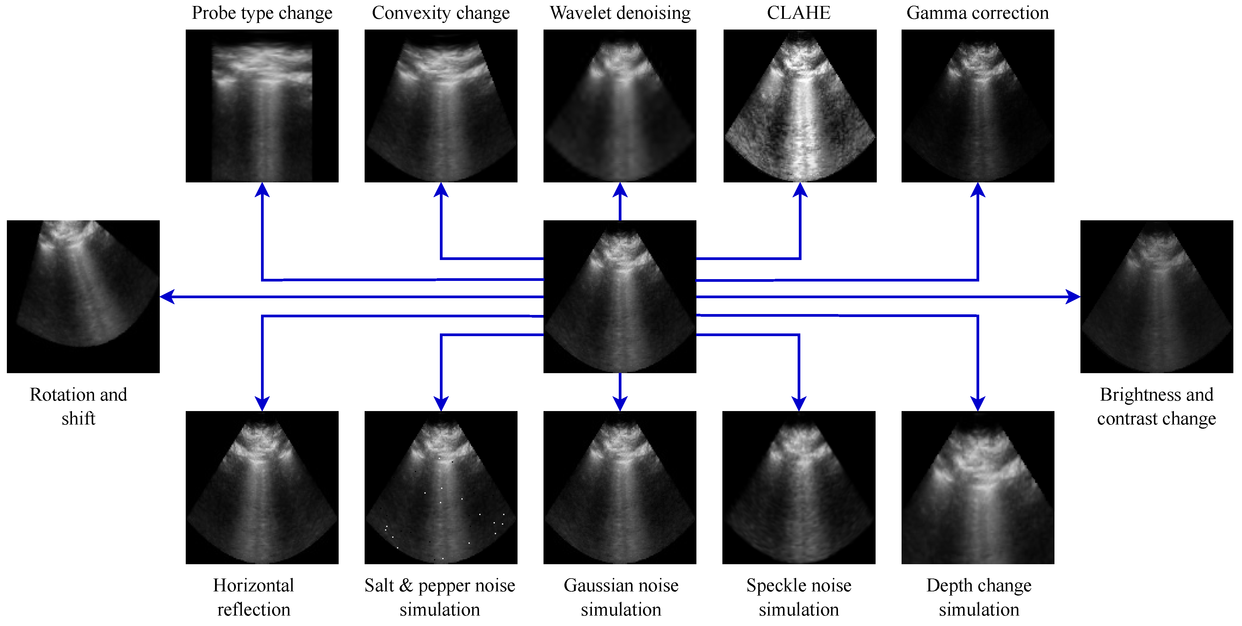
Figure 3.
Examples of ultrasound-specific data augmentation transformations applied to the same ultrasound image.
Figure 3.
Examples of ultrasound-specific data augmentation transformations applied to the same ultrasound image.
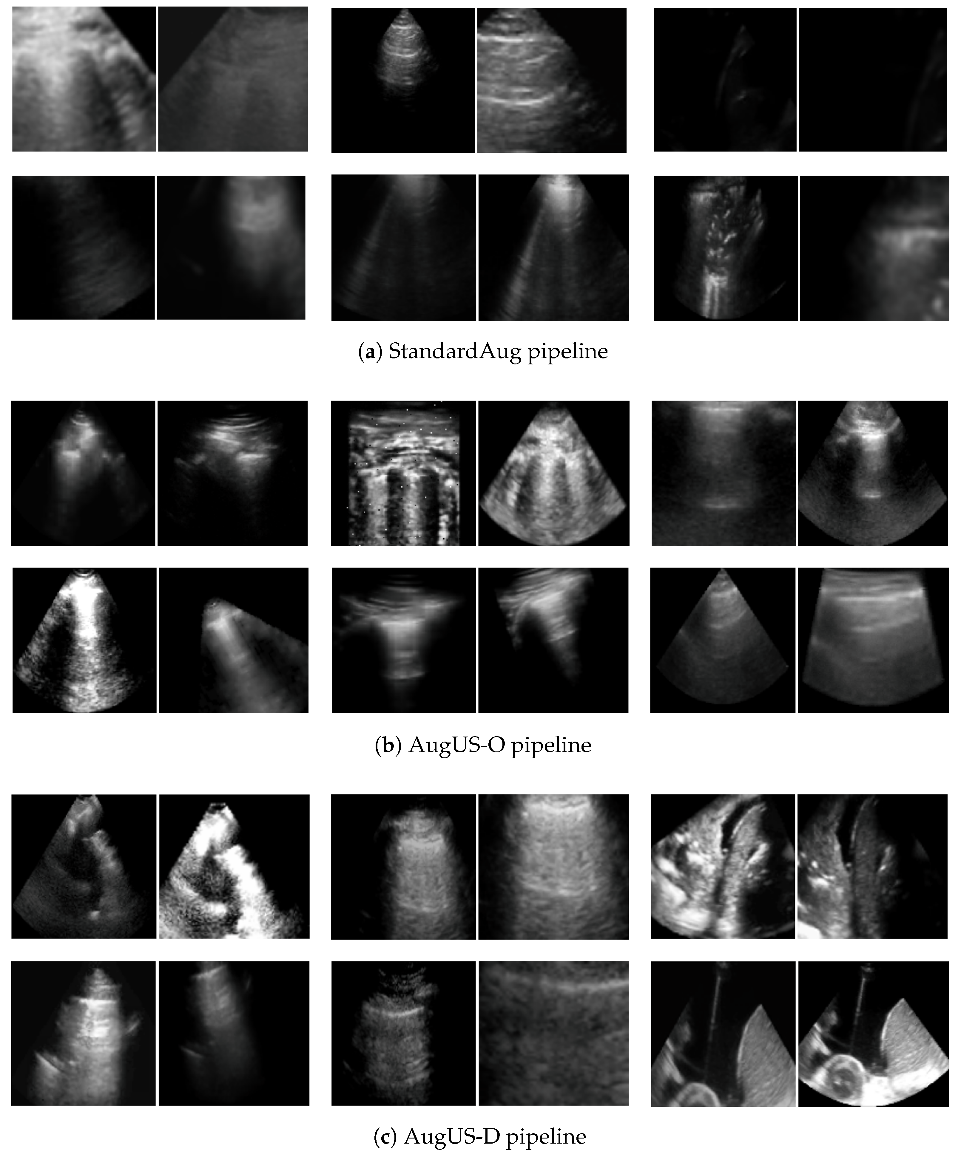
Figure 4.
Examples of positive pairs produced using each of the (a) StandardAug, (b) AugUS-O, and (c) AugUS-D data augmentation pipelines.
Figure 4.
Examples of positive pairs produced using each of the (a) StandardAug, (b) AugUS-O, and (c) AugUS-D data augmentation pipelines.
Figure 5.
Two-dimensional t-distributed Stochastic Neighbour Embeddings (t-SNEs) for test set feature vectors produced by SimCLR-pretrained backbones, for all tasks and data augmentation pipelines.
Figure 5.
Two-dimensional t-distributed Stochastic Neighbour Embeddings (t-SNEs) for test set feature vectors produced by SimCLR-pretrained backbones, for all tasks and data augmentation pipelines.
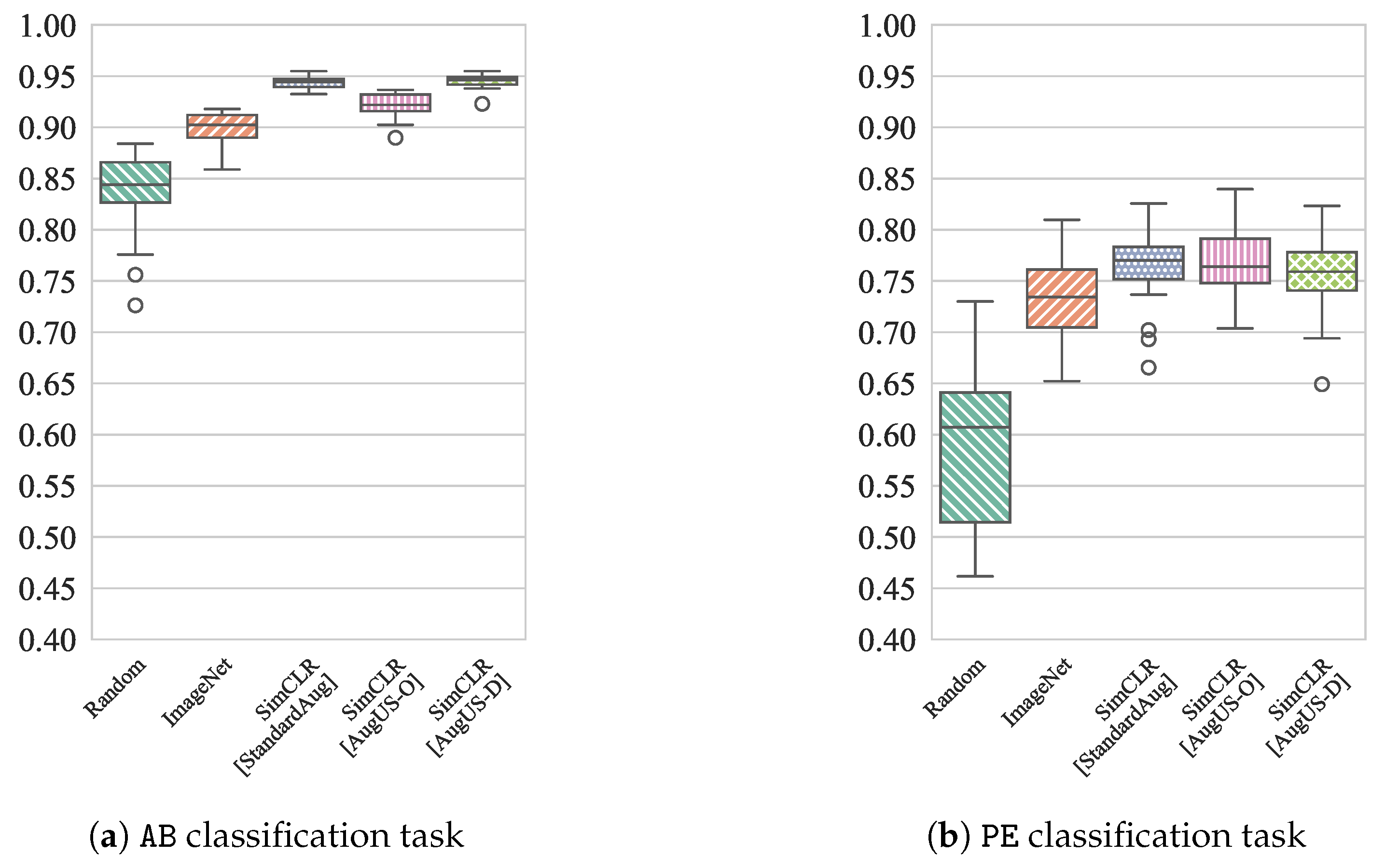
Figure 6.
Distribution of test AUC for classifiers trained on disjoint subsets of of the patients in the training partition of LUSData for (a) the AB task and (b) the PE task.
Figure 6.
Distribution of test AUC for classifiers trained on disjoint subsets of of the patients in the training partition of LUSData for (a) the AB task and (b) the PE task.
Figure 7.
Examples of how the random crop and resize transformation (A00) can reduce semantic information. Original images are on the left, and two random crops of the image are on the right. Top: The original image contains a B-line (purple), which is visible in View 2 but not in View 1. The original image also contains instances of the pleural line (yellow) which are visible in View 1 but not in View 2. Bottom: The original image contains a pleural effusion (green), which is visible in View 1 but largely obscured in View 2.
Figure 8.
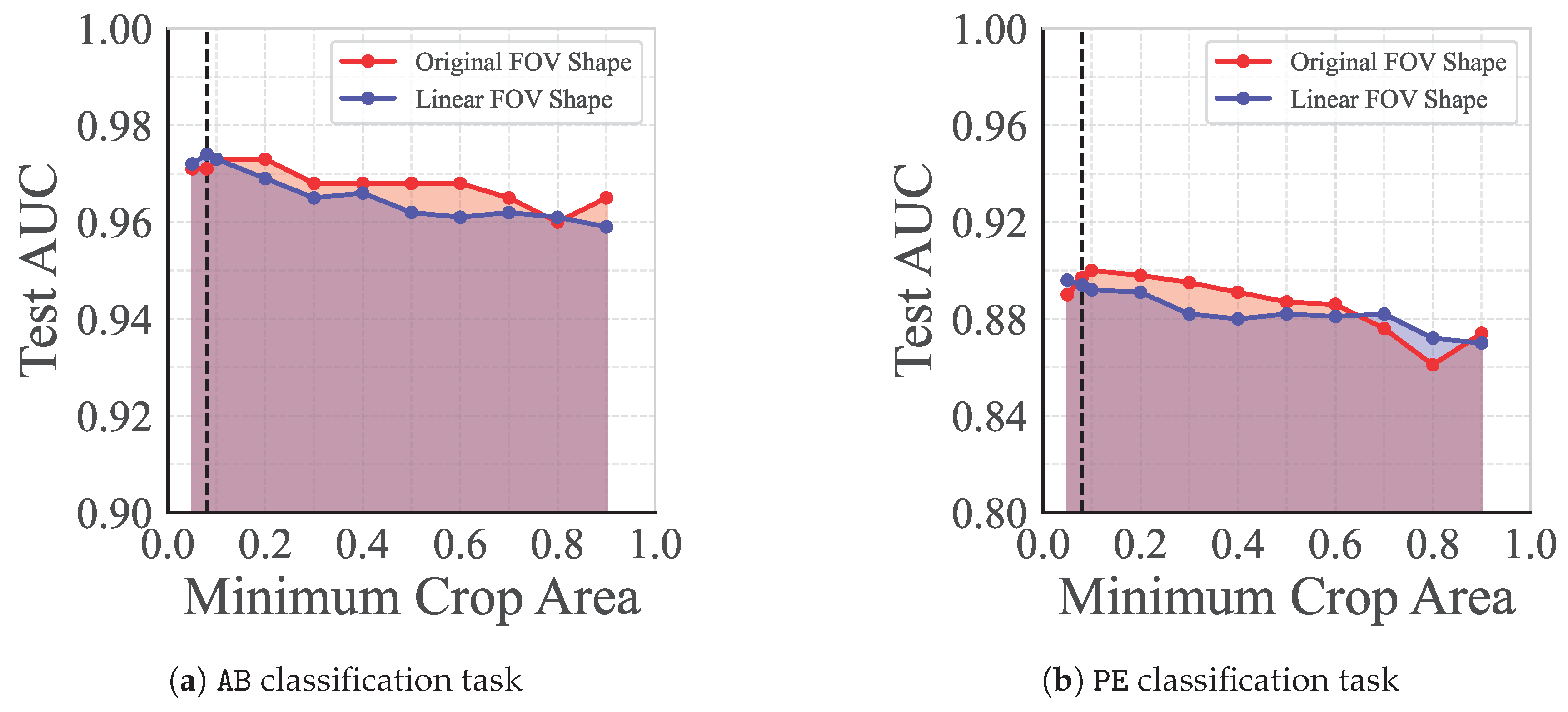
Test set AUC for linear classifiers trained on the representations outputted by pretrained backbones, for (a) the AB task and (b) the PE task. Each backbone was pretrained using AugUS-D with different values for the minimum crop area, c. Results are provided for models pretrained with the original ultrasound FOV, along with images transformed to linear field of view (FOV) only. The dashed line indicates the default value of .
Table 1.
Breakdown of the unlabelled, training, validation, and test sets in the private dataset. For each split, we indicate the number of distinct patients, videos, and images. indicates the number of labelled videos in the negative and positive class for each binary classification task. For the PL task, we indicate the number of videos with frame-level bounding box annotations.
| | Local | External |
|---|
| Unlabelled | Train | Validation | Test | Test |
|---|
| Patients | 5571 | 1702 | 364 | 364 | 168 |
| Videos | 59,309 | 5679 | 1184 | 1249 | 925 |
| Images | 1.3 × 10⁷ | 1.2 × 10⁶ | 2.5 × 10⁵ | 2.6 × 10⁵ | 1.1 × 10⁵ |
| AB labels | N/A | | | | |
| PE labels | N/A | | | | |
| PL labels | N/A | 200 | 39 | 45 | 0 |
Table 2.
The sequence of transformations in the StandardAug data augmentation pipeline.
Table 2.
The sequence of transformations in the StandardAug data augmentation pipeline.
| Identifier | Probability | Transformation | Time [ms] |
|---|
| A00 | 1.0 | Crop and resize | |
| A01 | 0.5 | Horizontal reflection | |
| A02 | 0.8 | Colour jitter. | |
| A03 | 0.2 | Conversion to grayscale | |
| A04 | 0.5 | Gaussian blur | |
| A05 | 0.1 | Solarization | |
Table 3.
The sequence of transformations in the ultrasound-specific augmentation pipeline.
Table 3.
The sequence of transformations in the ultrasound-specific augmentation pipeline.
| Identifier | Probability | Transformation | Time [ms] |
|---|
| B00 | 0.3 | Probe type change | |
| B01 | 0.75 | Convexity change | |
| B02 | 0.5 | Wavelet denoising | |
| B03 | 0.2 | CLAHE † | |
| B04 | 0.5 | Gamma correction | |
| B05 | 0.5 | Brightness and contrast change | |
| B06 | 0.5 | Depth change simulation | |
| B07 | 0.333 | Speckle noise simulation | |
| B08 | 0.333 | Gaussian noise | |
| B09 | 0.1 | Salt and pepper noise | |
| B10 | 0.5 | Horizontal reflection | |
| B11 | 0.5 | Rotation and shift | |
Table 4.
A comparison of ablated versions of the StandardAug and AugUS-O pipeline, with one excluded transformation versus the original pipelines. Models were pretrained on the LUSData unlabelled set and evaluated on two downstream classification tasks—AB and PE. Performance is expressed as mean and median test area under the receiver operating characteristic curve (AUC) from 10-fold cross-validation achieved by a linear classifier trained on the feature vectors of a frozen backbone.
| Pipeline | Omitted | AB | PE |
|---|
| | | Mean (std) | Median | Mean | Median |
|---|
| StandardAug | None | | | | |
| A00 | |
† | |
† |
| A01 | | | | |
| A02 | |
† | |
† |
| A03 | | | | |
| A04 | | | | |
| A05 | | | | |
| AugUS-O | None | | | | |
| B00 | | | | |
| B01 | | | | |
| B02 | |
§ | | |
| B03 | |
† | | |
| B04 | | | | |
| B05 | | | | |
| B06 | | | | |
| B07 | | | | |
| B08 | |
§ | | |
| B09 | |
§ | | |
| B10 | | | | |
| B11 | |
† | | |
Table 5.
Test set performance for linear classification (LC) and fine-tuning (FT) experiments with the AB and PE tasks. Binary metrics are averages across classes. The best observed metrics in each experimental setting are in boldface.
Table 5.
Test set performance for linear classification (LC) and fine-tuning (FT) experiments with the AB and PE tasks. Binary metrics are averages across classes. The best observed metrics in each experimental setting are in boldface.
Train
Setting | Task | Initial
Weights | Pipeline | Accuracy | Precision | Recall | AUC |
|---|
| LC | AB | SimCLR | StandardAug | | | | |
| SimCLR | AugUS-O | | | | |
| SimCLR | AugUS-D | | | | |
| ImageNet | - | | | | |
| PE | SimCLR | StandardAug | | | | |
| SimCLR | AugUS-O | | | | |
| SimCLR | AugUS-D | | | | |
| ImageNet | - | | | | |
| FT | AB | SimCLR | StandardAug | | | | |
| SimCLR | AugUS-O | | | | |
| SimCLR | AugUS-D | | | | |
| Random | - | | | | |
| ImageNet | - | | | | |
| PE | SimCLR | StandardAug | | | | |
| SimCLR | AugUS-O | | | | |
| SimCLR | AugUS-D | | | | |
| Random | - | | | | |
| ImageNet | - | | | | |
Table 6.
External test set metrics for linear classification (LC) and fine-tuning (FT) experiments with the AB and PE tasks. Binary metrics are averages across classes. The best observed metrics in each experimental setting are in boldface.
Table 6.
External test set metrics for linear classification (LC) and fine-tuning (FT) experiments with the AB and PE tasks. Binary metrics are averages across classes. The best observed metrics in each experimental setting are in boldface.
Train
Setting | Task | Initial
Weights | Pipeline | Accuracy | Precision | Recall | AUC |
|---|
| LC | AB | SimCLR | StandardAug | | | | |
| SimCLR | AugUS-O | | | | |
| SimCLR | AugUS-D | | | | |
| ImageNet | - | | | | |
| PE | SimCLR | StandardAug | | | | |
| SimCLR | AugUS-O | | | | |
| SimCLR | AugUS-D | | | | |
| ImageNet | - | | | | |
| FT | AB | SimCLR | StandardAug | | | | |
| SimCLR | AugUS-O | | | | |
| SimCLR | AugUS-D | | | | |
| Random | - | | | | |
| ImageNet | - | | | | |
| PE | SimCLR | StandardAug | | | | |
| SimCLR | AugUS-O | | | | |
| SimCLR | AugUS-D | | | | |
| Random | - | | | | |
| ImageNet | - | | | | |
Table 7.
Test set performance for linear classification (LC) and fine-tuning (FT) experiments with the COVID task. Binary metrics are averages across classes. The best observed metrics in each experimental setting are in boldface.
Table 7.
Test set performance for linear classification (LC) and fine-tuning (FT) experiments with the COVID task. Binary metrics are averages across classes. The best observed metrics in each experimental setting are in boldface.
Train
Setting | Pretraining
Dataset | Initial
Weights | Pipeline | Accuracy | Precision | Recall | AUC |
|---|
| LC | LUSData | SimCLR | StandardAug | | | | |
| SimCLR | AugUS-O | | | | |
| SimCLR | AugUS-D | | | | |
| COVIDx-US | SimCLR | StandardAug | | | | |
| SimCLR | AugUS-O | | | | |
| SimCLR | AugUS-D | | | | |
| - | ImageNet | - | | | | |
| FT | LUSData | SimCLR | StandardAug | | | | |
| SimCLR | AugUS-O | | | | |
| SimCLR | AugUS-D | | | | |
| COVIDx-US | SimCLR | StandardAug | | | | |
| SimCLR | AugUS-O | | | | |
| SimCLR | AugUS-D | | | | |
| - | Random | - | | | | |
| - | ImageNet | - | | | | |
Table 8.
LUSData local test set AP@50 for the PL task observed for SSD models whose backbones were pretrained using different data augmentation pipelines. Boldface values indicate top performance.
Table 8.
LUSData local test set AP@50 for the PL task observed for SSD models whose backbones were pretrained using different data augmentation pipelines. Boldface values indicate top performance.
| Backbone | Initial Weights | Pipeline | AP@50 |
|---|
| Frozen | SimCLR | StandardAug | |
| SimCLR | AugUS-O | |
| SimCLR | AugUS-D | |
| Random | - | |
| ImageNet | - | |
| Trainable | SimCLR | StandardAug | |
| SimCLR | AugUS-O | |
| SimCLR | AugUS-D | |
| Random | - | |
| ImageNet | - | |
Table 9.
Test set AUC for SimCLR-pretrained models with (✓) and without (✗) semantics-preserving preprocessing. Results are reported for linear classifiers and fine-tuned models.
Table 9.
Test set AUC for SimCLR-pretrained models with (✓) and without (✗) semantics-preserving preprocessing. Results are reported for linear classifiers and fine-tuned models.
| | | Linear Classifier | Fine-Tuned |
|---|
| Task | Pipeline/Preprocessing | ✗ | ✓ | ✗ | ✓ |
|---|
| AB | StandardAug | | | | |
| AugUS-O | | | | |
| AugUS-D | | | | |
| PE | StandardAug | | | | |
| AugUS-O | | | | |
| AugUS-D | | | | |
| COVID | StandardAug | | | | |
| AugUS-O | | | | |
| AugUS-D | | | | |
