Author Contributions
Conceptualization, S.D. (Sivanesan Dakshanamurthy); Methodology, A.K., M.S., H.G., J.M., S.D. (Somanath Dandibhotla) and S.D. (Sivanesan Dakshanamurthy); Software, A.K., M.S., S.D. (Somanath Dandibhotla) and S.D. (Sivanesan Dakshanamurthy); Validation, A.K.; Formal analysis, A.K.; Investigation, A.K., M.S., H.G., J.M. and S.D. (Somanath Dandibhotla); Resources, S.D. (Sivanesan Dakshanamurthy); Data curation, A.K., M.S. and S.D. (Somanath Dandibhotla); Writing—original draft, A.K., M.S., H.G., J.M., S.D. (Somanath Dandibhotla) and S.D. (Sivanesan Dakshanamurthy); Writing—review & editing, A.K., M.S., H.G., J.M., S.D. (Somanath Dandibhotla) and S.D. (Sivanesan Dakshanamurthy); Supervision, S.D. (Sivanesan Dakshanamurthy); Project administration, S.D. (Sivanesan Dakshanamurthy); Funding acquisition, S.D. (Sivanesan Dakshanamurthy) All authors have read and agreed to the published version of the manuscript.
Figure 1.
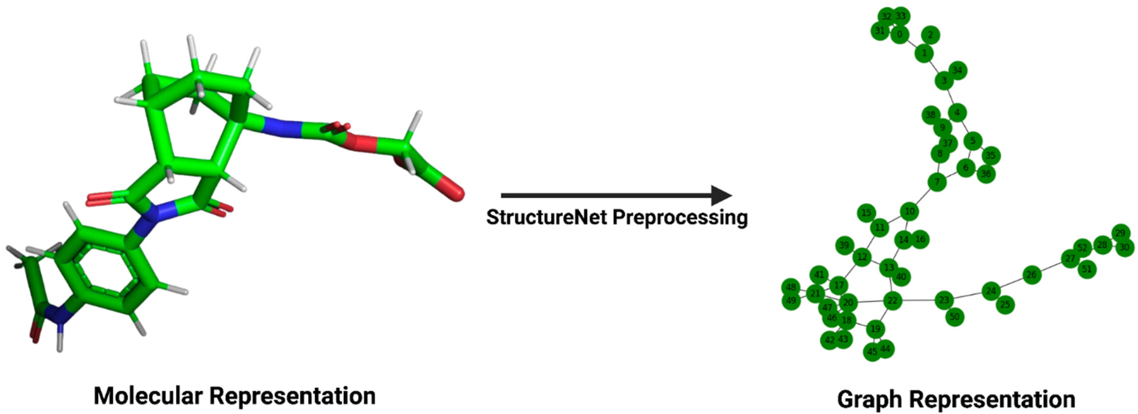
Transformation of a molecular structure into its graph representation. The left panel depicts the structure of a ligand, viewed in PyMOL (version 2.5.5), from its .pdb file in the PDBBind v2020 refined set. The right panel depicts the same ligand’s graph representation for input into StructureNet.
Figure 1.
Transformation of a molecular structure into its graph representation. The left panel depicts the structure of a ligand, viewed in PyMOL (version 2.5.5), from its .pdb file in the PDBBind v2020 refined set. The right panel depicts the same ligand’s graph representation for input into StructureNet.
Figure 2.
Visualization of node, edge, and graph feature calculations. (A) Nodes and edges in StructureNet graphs represent atom and bond-level properties, respectively. (B) Graph-level features in StructureNet graphs represent global molecule-level characteristics.
Figure 2.
Visualization of node, edge, and graph feature calculations. (A) Nodes and edges in StructureNet graphs represent atom and bond-level properties, respectively. (B) Graph-level features in StructureNet graphs represent global molecule-level characteristics.
Figure 3.
The training and testing framework for StructureNet. The protein–ligand graph and molecular features enter the GNN through GeneralConv and Linear layers, respectively. After GNN processing, they are combined and used to train XGBoost and SVM simultaneously. Predictions from SVM and XGBoost are generated, combined, and fed to linear regression to generate final predictions. All GNN layers used MAE as the loss function and Adam as the optimizer to update weights.
Figure 4.
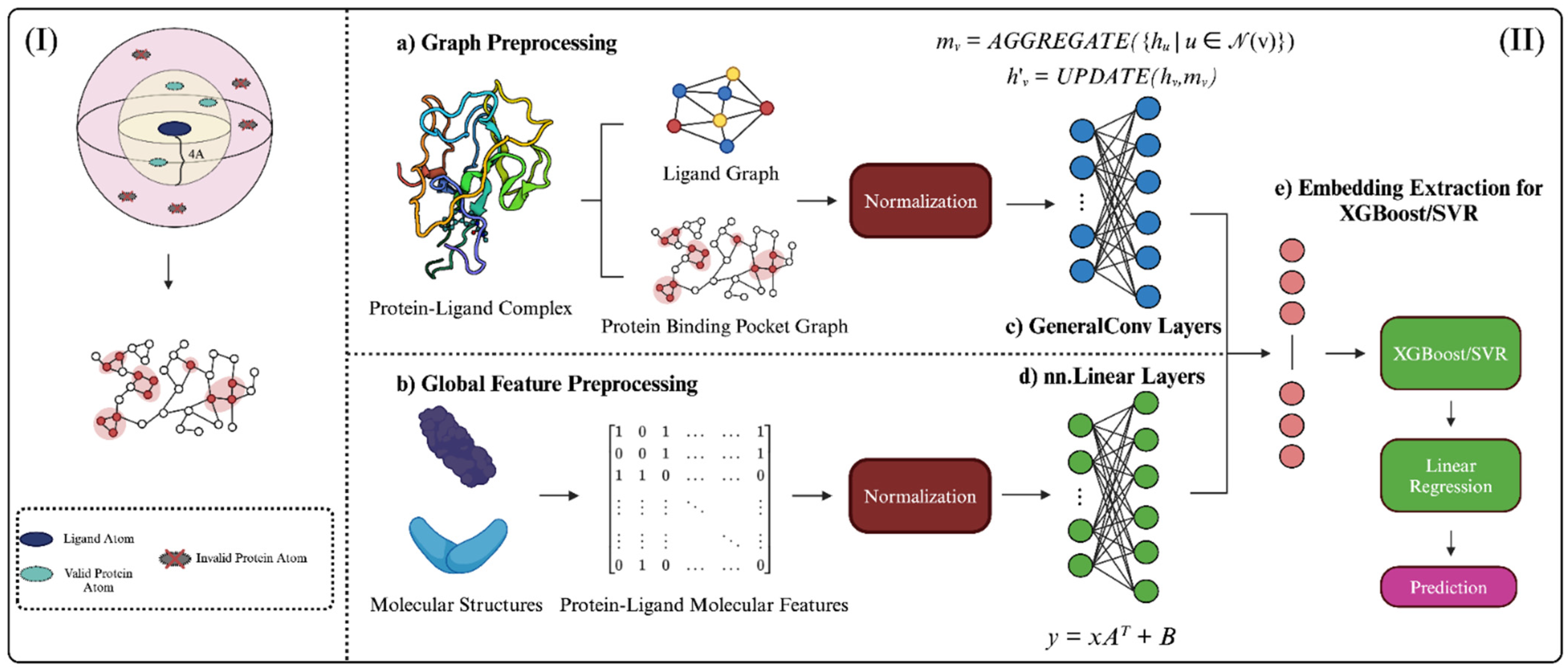
Graphical abstract depicting StructureNet workflow, from data preparation to binding affinity prediction. (I) Visual representation of the distance cutoff employed in protein binding pocket graphs. Pocket atoms >4 Å from the ligand were not considered. (II) The overall workflow of StructureNet in the broader context of other connected processes. (a) Each protein–ligand complex file from the respective PDBBind dataset was processed to generate a protein-binding pocket graph, ligand graph, (b) and protein–ligand molecular feature vector. Features were normalized using min–max normalization. Normalized graphs were inputted into the GNN (c,d) and concatenated to form a single input, after which embeddings were extracted and fed through SVR/XGBoost and linear regression to generate predictions (e).
Figure 4.
Graphical abstract depicting StructureNet workflow, from data preparation to binding affinity prediction. (I) Visual representation of the distance cutoff employed in protein binding pocket graphs. Pocket atoms >4 Å from the ligand were not considered. (II) The overall workflow of StructureNet in the broader context of other connected processes. (a) Each protein–ligand complex file from the respective PDBBind dataset was processed to generate a protein-binding pocket graph, ligand graph, (b) and protein–ligand molecular feature vector. Features were normalized using min–max normalization. Normalized graphs were inputted into the GNN (c,d) and concatenated to form a single input, after which embeddings were extracted and fed through SVR/XGBoost and linear regression to generate predictions (e).
Figure 5.
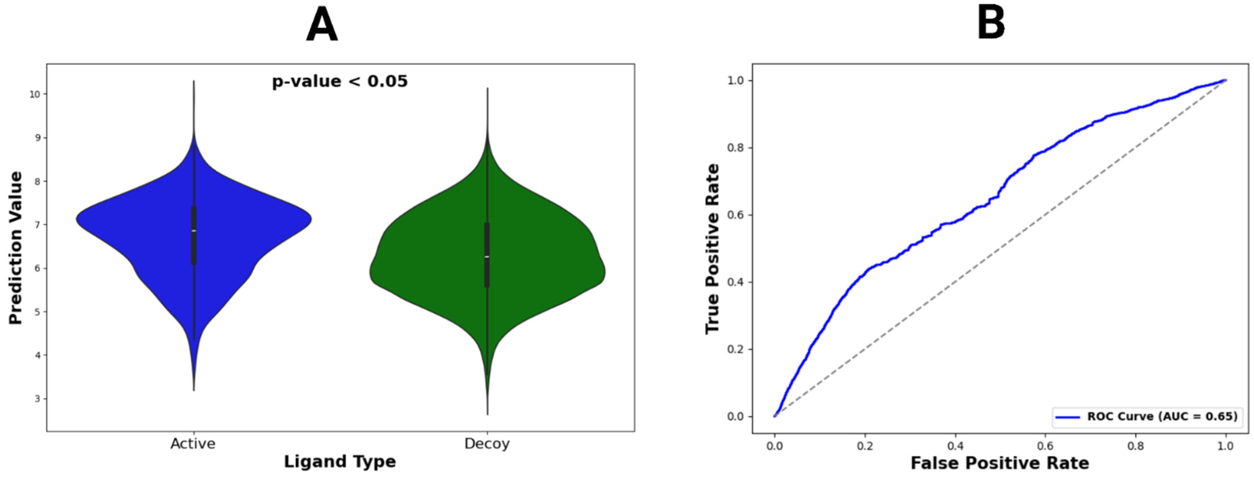
Violin plot and ROC curve for DUDE-Z dataset predictions. (A) The violin plot constructed for active vs. decoy ligands across all DUDE-Z complexes. Locations with wider color densities indicate higher frequencies of predictions. A p-value was calculated from t-tests comparing mean binding affinity predictions between active and decoy ligands. (B) The ROC curve, representing all predictions, with its AUC value given in the legend.
Figure 5.
Violin plot and ROC curve for DUDE-Z dataset predictions. (A) The violin plot constructed for active vs. decoy ligands across all DUDE-Z complexes. Locations with wider color densities indicate higher frequencies of predictions. A p-value was calculated from t-tests comparing mean binding affinity predictions between active and decoy ligands. (B) The ROC curve, representing all predictions, with its AUC value given in the legend.
Figure 6.
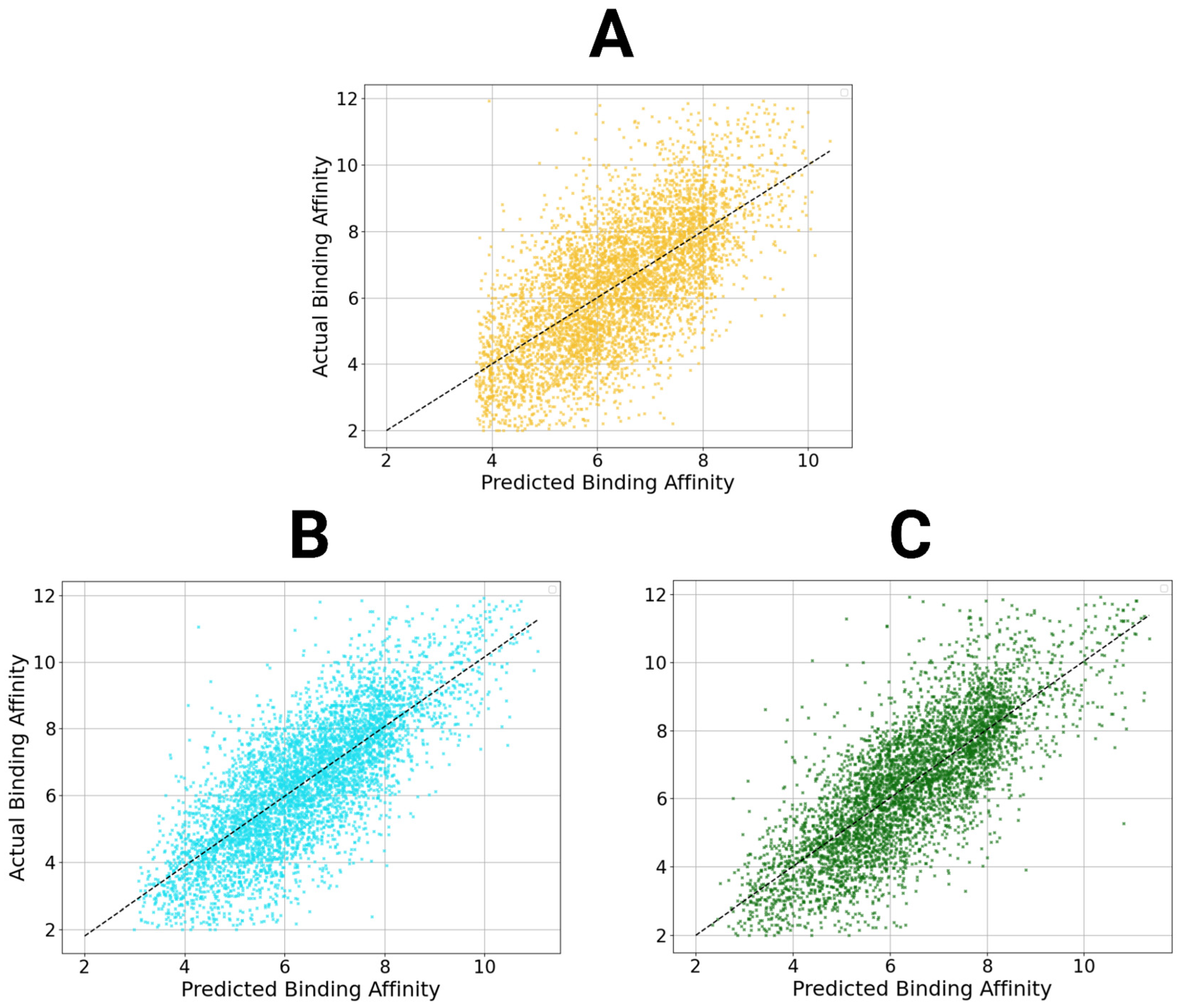
Scatter plots of StructureNet and hybridized model predictions. Scatter plots of the predictions from StructureNet (A), Structure + Sequence V2 (STR + SEQ, (B)), and Structure + Interaction V2 (STR + INT, (C)) against actual binding affinity values.
Figure 6.
Scatter plots of StructureNet and hybridized model predictions. Scatter plots of the predictions from StructureNet (A), Structure + Sequence V2 (STR + SEQ, (B)), and Structure + Interaction V2 (STR + INT, (C)) against actual binding affinity values.
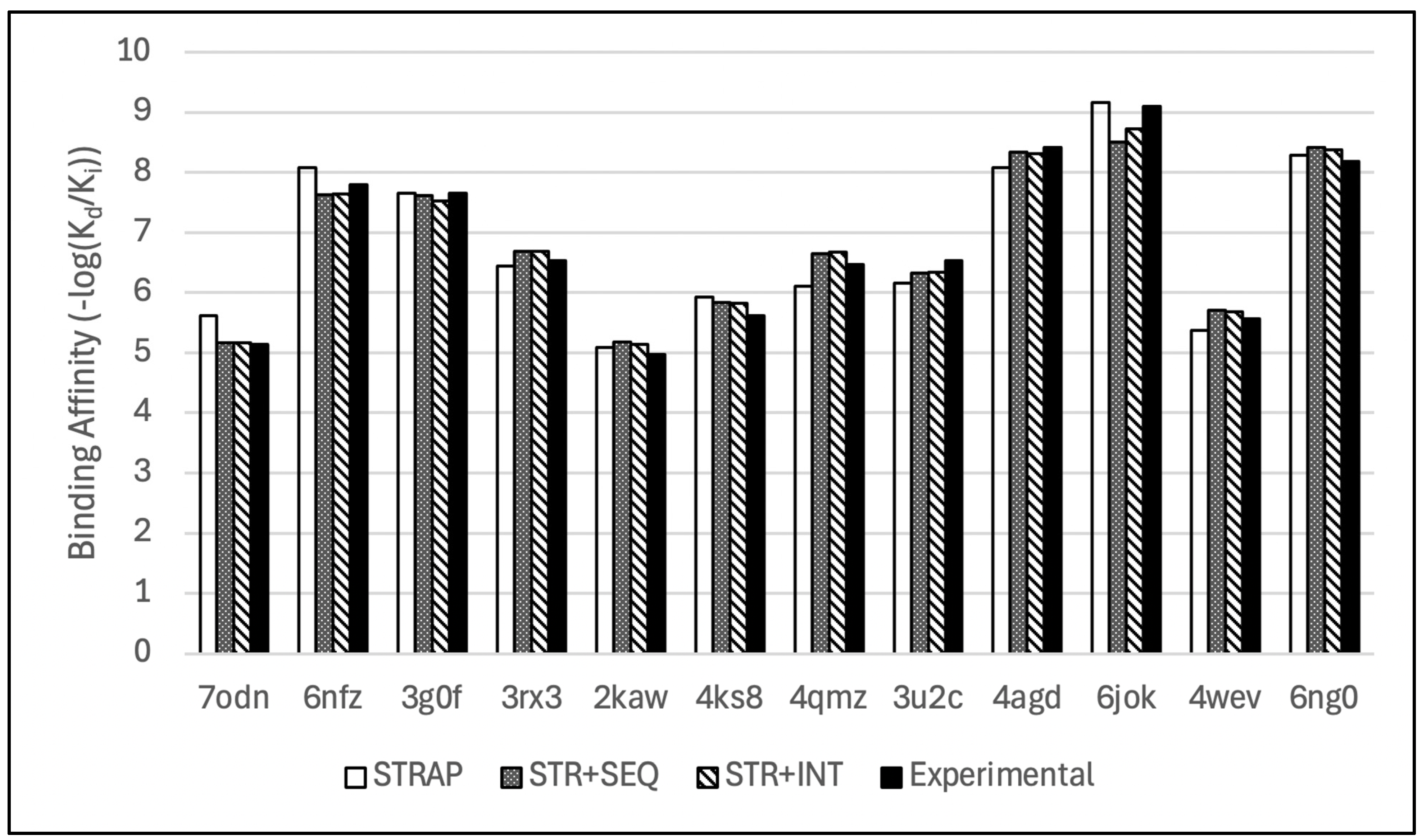
Figure 7.
Bar chart comparison of de novo binding affinity predictions from the hybridized models with their respective experimental values.
Figure 7.
Bar chart comparison of de novo binding affinity predictions from the hybridized models with their respective experimental values.
Figure 8.
Trendlines showing the relationship between model predictions (StructureNet, StructureNet + Int, StructureNet + Seq, StructureNet + Seq + Int, AutoDock Vina) and experimental binding affinity values. Twelve docked complexes were used to generate binding affinity values, which were converted to −log(Kd) for smoothness of fit. The purple dotted line is a reference line representing the experimental binding affinity values and a perfect linear correlation.
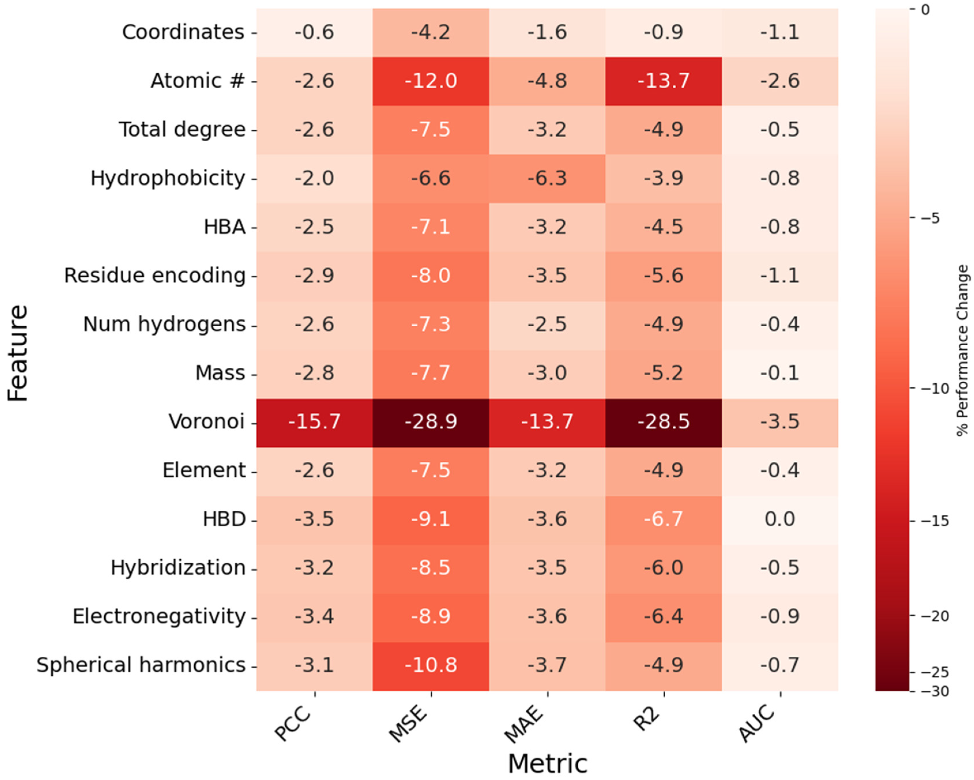
Figure 9.
Heatmap showing the impact of node feature removal on model PCC, MSE, MAE, R2, and AUC. Each cell represents the percent difference from baseline value for a given metric (column) when the corresponding feature (row) is removed. Cells are assigned a value, as a percentage (%), and a color, which is determined by the magnitude of the percent difference.
Figure 10.
(A) Scatter plot with trendline showing the distribution of the exemplary conformer’s binding affinity predictions across the duration of its MD simulation. The data point representing the most accurate prediction is given above in orange. (B) Scatter plots for all other conformer ensembles in the dataset. The data points representing the most accurate predictions are given above in red.
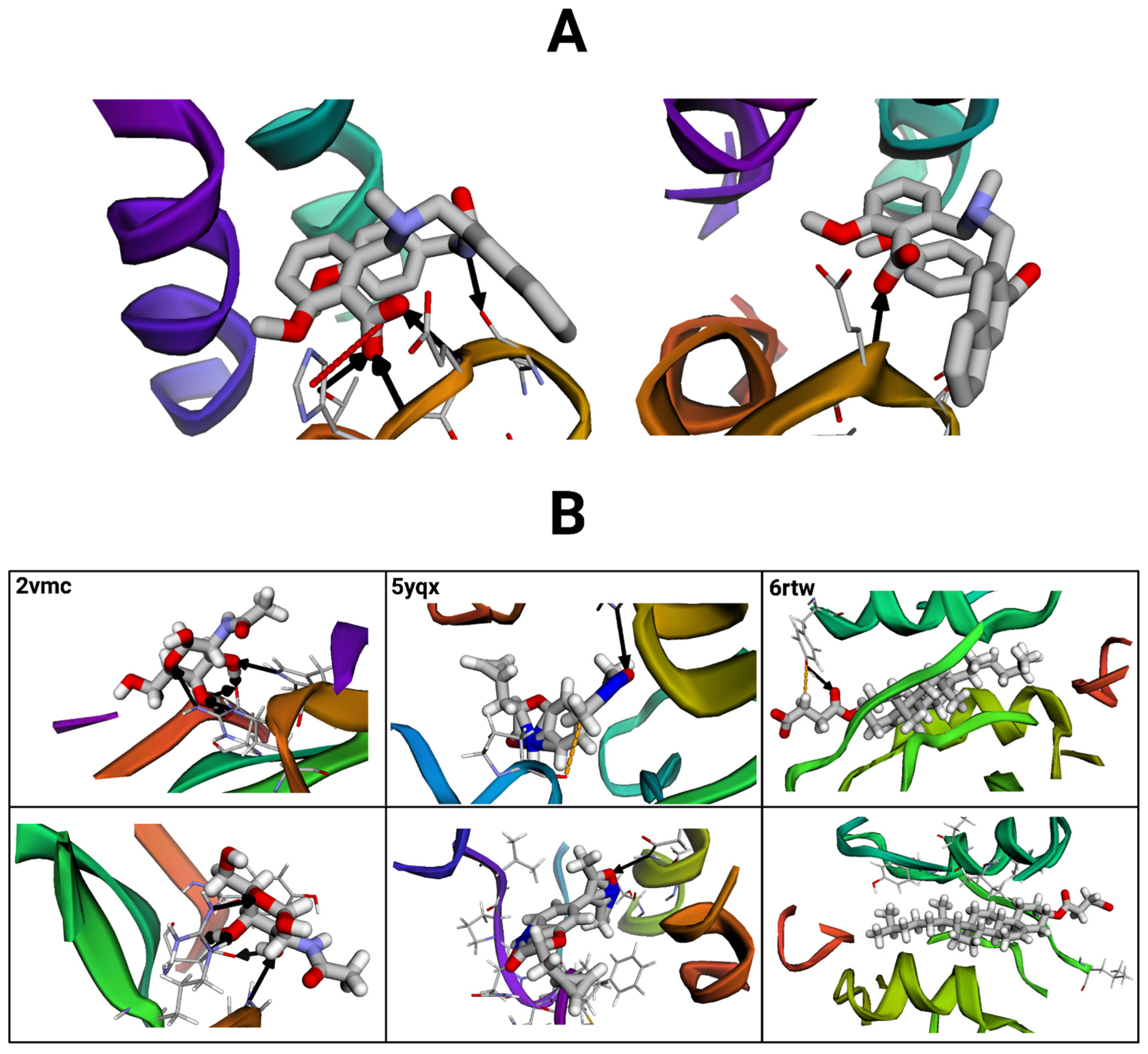
Figure 11.
Protein–ligand complex interactions visualized with the BINANA (version 2.2) online software. Black arrows represent hydrogen bonds, red dashed lines depict salt bridges, and orange dashed lines represent metal contacts. (A) Visualization of the exemplary reference structure (left) compared to a selected conformer. Molecular files were dehydrogenated and maximized for clarity. (B) Visualizations of three additional reference structure–conformer pairs (paired vertically). Images on the top represent reference structures, and those below represent their conformer pairs.
Table 1.
Node and edge features used to represent protein-binding pocket and ligand structures in graphs. Descriptors in nodes and edges detail atom- and bond-related properties, respectively.
Table 1.
Node and edge features used to represent protein-binding pocket and ligand structures in graphs. Descriptors in nodes and edges detail atom- and bond-related properties, respectively.
| Feature Name | Feature Description |
|---|
| Atomic number | The element’s atomic number. |
| Total degree | Total number of bonds formed with other atoms. |
| Hybridization | The atom’s hybridization state. |
| Total number of hydrogens | The total number of hydrogens bonded to the atom. |
| Mass | The atom’s atomic mass. |
| Hydrogen bond donor * | The atom’s hydrogen bond donor status. |
| Hydrogen bond acceptor * | The atom’s hydrogen bond acceptor status. |
| Hydrophobicity index * | The atom’s hydrophobicity. |
| Electronegativity * | The atom’s electronegativity. |
| Element name * | The element’s chemical abbreviation. |
| Residue encoding * | One-hot encoding of the residue type (amino acid for protein atoms, other for ligand atoms). |
| Voronoi regions * | Constructs a Voronoi diagram and calculates spatial relationships between atoms. |
| Spherical harmonics * | Calculates angular properties of the atomic coordinates in ℝ3. |
| Coordinate list * | The Cartesian coordinates of the atom in ℝ3 (x, y, z). |
| Bond type | The type of bond represented by an edge. |
| Conjugation status | Whether a bond is part of a conjugated system. |
| Ring status | Whether a bond is part of a cyclic ring structure. |
| Bond order * | The number of chemical bonds between two atoms. |
| Bond length * | The length of a bond between two atoms. |
| Electrostatic interactions * | The Coulombic attraction/repulsion between two charged atoms. |
Table 2.
Molecular features included in protein-binding pocket and ligand graphs. Unlike node (atom) and edge (bond) features, these molecular features represent global molecule-level characteristics and are stored as graph-level attributes.
Table 2.
Molecular features included in protein-binding pocket and ligand graphs. Unlike node (atom) and edge (bond) features, these molecular features represent global molecule-level characteristics and are stored as graph-level attributes.
| Feature Name | Feature Description |
|---|
| Asphericity | Calculates molecular asphericity. |
| Eccentricity | Calculates molecular eccentricity. |
| exact molecular weight | Describes exact molecular weight. |
| CSP3 | Describes the number of C atoms that are SP3 hybridized. |
| Inertial shape factor | Describes molecular inertial shape factor. |
| Number of aliphatic carbocycles | Calculates the number of aliphatic carbocycles for a molecule. |
| Number of amide bonds | Calculates the number of amide bonds within a molecule. |
| Number of aromatic carbocycles | Calculates the number of aromatic carbocycles for a molecule. |
| Hall–Kier alpha | Measures the degree of connectivity and branching within a molecule. |
| H-bond acceptors | Calculates the number of hydrogen bond acceptors for a molecule. |
| H-bond donors | Calculates the number of hydrogen bond donors for a molecule. |
| Heteroatoms | Calculates the number of non-carbon atoms in a molecule. |
| Rotatable bonds | Calculates the number of rotatable bonds in a molecule. |
| MolLogP * | Calculates the lipophilicity of a ligand (0 for protein). |
| NHOH count * | Calculates the number of amine and hydroxyl groups in a molecule. |
| NO count * | Calculates the number of nitrogen and oxygen atoms in a molecule. |
| QED * | Calculates the quantitative estimate of drug-likeness for a molecule. |
| PEOE_VSA1-14 | Calculates the partial equalization of orbital electronegativities for a molecule. |
| SMR_VSA1-8 | Measures the Van der Waals surface of a molecule categorized by ranges of molar refractivity. |
| SlogP_VSA1-12 | Measures the Van der Waals surface of a molecule as divided into regions based on logP values. |
| VSA_EState1-10 | Measures the Van der Waals surface of a molecule as divided into regions based on electrostatic state indices. |
| MolMR | Calculates the molar refractivity of a molecule. |
| TPSA | Returns a molecule’s TPSA value. |
| Kappa1 | Calculates molecular Hall–Kier kappa1 value. |
| LabuteASA | Calculates Labute’s approximate surface area for the molecule. |
| PBF | Returns the plane of best fit (PBF) for a molecule. |
| Chi0n/v | Calculates the chi index of a molecule that characterizes its structural attributes. |
| Morgan fingerprint | Describes the surrounding environments/substructures of atoms in a molecular fingerprint. |
| Hashed torsion topological fingerprint | Describes the torsion angles in a molecular fingerprint. |
| Hashed atom pair fingerprint | Describes the shortest paths between bonded atoms in a molecular fingerprint. |
Table 3.
Search space of hyperparameters tested for the StructureNet model architecture. Hyperparameters chosen by Hyperopt and used for StructureNet are given in bold.
Table 3.
Search space of hyperparameters tested for the StructureNet model architecture. Hyperparameters chosen by Hyperopt and used for StructureNet are given in bold.
| Hyperparameter | Search Space |
|---|
| Hidden channels | 64, 128, 256 |
| Optimizer | Adam, Adagrad, RMSProp, Huber |
| Hidden layers | 2, 3, 4, 5 |
| Learning rate | 0.005, 0.001, 0.05, 0.01 |
| Loss function | MSE, MAE |
| Dropout rate | 0.3, 0.4, 0.5 |
| Edge dropout rate | 0.05, 0.1, 0.5 |
| Batch size | 32, 64, 128, 256 |
| Epochs | 50, 75, 100 |
Table 4.
Predictive power of StructureNet on the PDBBind v2020 refined set.
Table 4.
Predictive power of StructureNet on the PDBBind v2020 refined set.
| Fold | MSE | MAE | R2 | PCC | AUC |
|---|
| Average | 1.964 | 1.125 | 0.466 | 0.683 | 0.750 |
| Fold 1 | 1.887 | 1.119 | 0.458 | 0.677 | 0.713 |
| Fold 2 | 1.958 | 1.135 | 0.466 | 0.683 | 0.777 |
| Fold 3 | 2.075 | 1.133 | 0.464 | 0.681 | 0.749 |
| Fold 4 | 2.025 | 1.151 | 0.466 | 0.683 | 0.728 |
| Fold 5 | 1.755 | 1.066 | 0.477 | 0.691 | 0.740 |
| Fold 6 | 2.057 | 1.151 | 0.461 | 0.679 | 0.752 |
| Fold 7 | 2.050 | 1.141 | 0.455 | 0.675 | 0.734 |
| Fold 8 | 1.899 | 1.109 | 0.479 | 0.692 | 0.755 |
Table 5.
StructureNet predictive power on the PDBBind v2020 general set.
Table 5.
StructureNet predictive power on the PDBBind v2020 general set.
| Fold | MSE | MAE | R2 | PCC | AUC |
|---|
| Average | 1.959 | 1.104 | 0.385 | 0.620 | 0.733 |
| Fold 1 | 1.960 | 1.116 | 0.388 | 0.623 | 0.726 |
| Fold 2 | 1.862 | 1.073 | 0.398 | 0.631 | 0.747 |
| Fold 3 | 1.983 | 1.113 | 0.386 | 0.621 | 0.727 |
| Fold 4 | 1.975 | 1.103 | 0.404 | 0.635 | 0.745 |
| Fold 5 | 1.957 | 1.102 | 0.382 | 0.618 | 0.726 |
| Fold 6 | 2.066 | 1.142 | 0.361 | 0.601 | 0.711 |
| Fold 7 | 1.873 | 1.074 | 0.383 | 0.619 | 0.737 |
| Fold 8 | 1.995 | 1.114 | 0.375 | 0.612 | 0.749 |
Table 6.
StructureNet predictive performance on the combined set.
Table 6.
StructureNet predictive performance on the combined set.
| Fold | MSE | MAE | R2 | PCC | AUC |
|---|
| Average | 1.956 | 1.107 | 0.416 | 0.645 | 0.738 |
| Fold 1 | 1.981 | 1.107 | 0.422 | 0.650 | 0.739 |
| Fold 2 | 1.959 | 1.117 | 0.402 | 0.634 | 0.724 |
| Fold 3 | 1.986 | 1.113 | 0.437 | 0.661 | 0.746 |
| Fold 4 | 1.928 | 1.109 | 0.422 | 0.635 | 0.745 |
| Fold 5 | 1.912 | 1.098 | 0.419 | 0.647 | 0.741 |
| Fold 6 | 1.995 | 1.120 | 0.415 | 0.644 | 0.731 |
| Fold 7 | 1.906 | 1.087 | 0.431 | 0.656 | 0.763 |
| Fold 8 | 1.995 | 1.115 | 0.380 | 0.617 | 0.729 |
Table 7.
StructureNet average predictive performance on external validation datasets.
Table 7.
StructureNet average predictive performance on external validation datasets.
| Model | MSE | MAE | R2 | PCC | AUC |
|---|
| StructureNet1 | 3.040 | 1.326 | 0.216 | 0.441 | 0.678 |
| StructureNet2 | 1.765 | 1.071 | 0.621 | 0.788 | 0.775 |
| StructureNet3 | 0.823 | 0.610 | 0.525 | 0.724 | 0.828 |
Table 8.
Comparison of existing structure-based graph neural network models for binding affinity prediction [
22].
Table 8.
Comparison of existing structure-based graph neural network models for binding affinity prediction [
22].
| Machine Learning Model | Binding Affinity Dataset | MSE | PCC |
|---|
| StructureNet | PDBBind v2020 Refined Set (n = 5316) | 1.991 | 0.682 |
| MPNN (PL) | PDBBind v2019 Hold-out (n = 3386) | 1.512 | 0.645 |
Table 9.
Comparison of successful deep learning models for binding affinity prediction [
5,
31,
32,
33,
34,
35].
Table 9.
Comparison of successful deep learning models for binding affinity prediction [
5,
31,
32,
33,
34,
35].
| Name | Feature Type(s) | Dataset | MSE | MAE | PCC |
|---|
| StructureNet | Structure | PDBBind v2020 Refined Set | 1.964 | 1.125 | 0.683 |
| StructureNet | Structure | PDBBind v2016 Core Set | 2.013 | 1.094 | 0.749 |
| StructureNet | Structure | PDBBind v2013 Core Set | 2.356 | 1.171 | 0.701 |
| Pafnucy | Structure, Sequence | PDBBind v2013 Core Set | 1.62 | N/A | 0.70 |
| DeepBindRG | Structure, Interaction | PDBBind v2013 Core Set | 3.302 | 1.483 | 0.639 |
| LigityScore | Structure, Interaction | PDBBind v2013 Core Set | 2.809 | 1.335 | 0.713 |
| LigityScore | Structure, Interaction | PDBBind v2016 Core Set | 2.277 | 1.224 | 0.725 |
| SIGN | Structure, Interaction | PDBBind v2016 Core Set | 1.836 | 1.027 | 0.797 |
| GraphBAR | Structure, Interaction | PDBBind v2016 Refined Set | 1.694 | 1.368 | 0.662 |
| HNN-denovo | Structure, Sequence, Interaction | PDBBind v2019 Refined Set | 0.922 | N/A | 0.840 |
Table 10.
Predictive performance of hybridizations between StructureNet and sequence- and interaction-based models. Two unique model versions (V1 and V2) were developed for both combinations of structural data with sequence and interaction data.
Table 10.
Predictive performance of hybridizations between StructureNet and sequence- and interaction-based models. Two unique model versions (V1 and V2) were developed for both combinations of structural data with sequence and interaction data.
| Model | MSE | MAE | R2 | PCC | AUC |
|---|
| Structural + Sequence − V1 | 1.701 | 1.025 | 0.530 | 0.743 | 0.761 |
| Structural + Sequence − V2 | 1.662 | 1.010 | 0.564 | 0.759 | 0.769 |
| Structural + Interaction − V1 | 1.680 | 1.018 | 0.561 | 0.751 | 0.767 |
| Structural + Interaction − V2 | 1.658 | 1.002 | 0.582 | 0.772 | 0.774 |
Table 11.
StructureNet predictions for an exemplary complex (PDB ID: 4g8n) and its ten conformers generated from MD simulations. The conformer with the most accurate prediction is bolded.
Table 11.
StructureNet predictions for an exemplary complex (PDB ID: 4g8n) and its ten conformers generated from MD simulations. The conformer with the most accurate prediction is bolded.
| Time Interval (ps) | Predicted Binding Affinity | Experimental Binding Affinity |
|---|
| 0 | 5.846 | 7.2 |
| 500 | 5.882 | 7.2 |
| 1000 | 5.908 | 7.2 |
| 1500 | 5.461 | 7.2 |
| 2000 | 5.461 | 7.2 |
| 2500 | 5.399 | 7.2 |
| 3000 | 5.305 | 7.2 |
| 3500 | 4.964 | 7.2 |
| 4000 | 5.482 | 7.2 |
| 4500 | 5.695 | 7.2 |
| 5000 | 5.130 | 7.2 |
Table 12.
StructureNet predictions vs. BINANA interaction calculations for an exemplary protein–ligand complex (PDB ID 4cig).
Table 12.
StructureNet predictions vs. BINANA interaction calculations for an exemplary protein–ligand complex (PDB ID 4cig).
| Complex Conformation | Predicted Binding Affinity | Experimental Binding Affinity | Total Protein–Ligand Interactions |
|---|
| Reference structure | 5.496 | 3.67 | 5 |
| Selected conformer | 4.929 | 3.67 | 1 |


 and
and 


