


A Radiomic Model for Gliomas Grade and Patient Survival Prediction

 ,
,  , ,
, ,
Abstract
1. Introduction
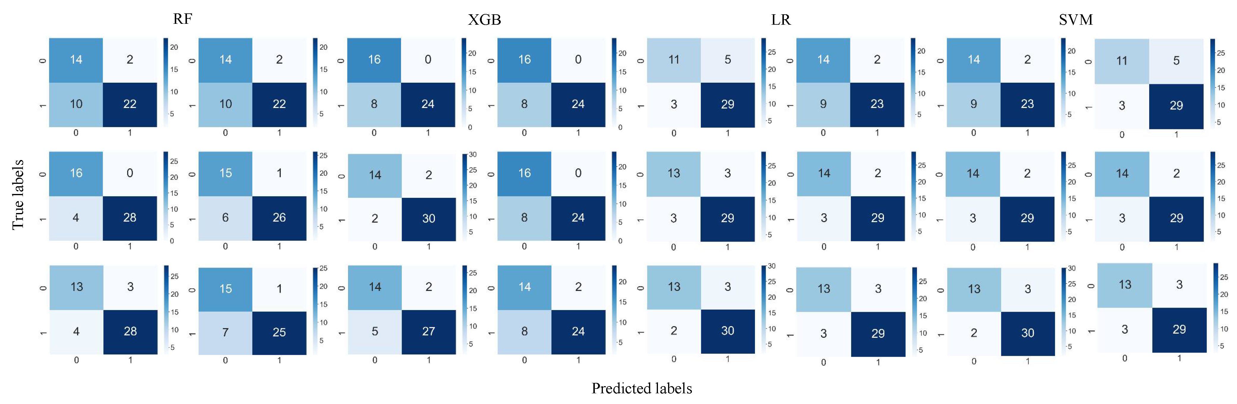
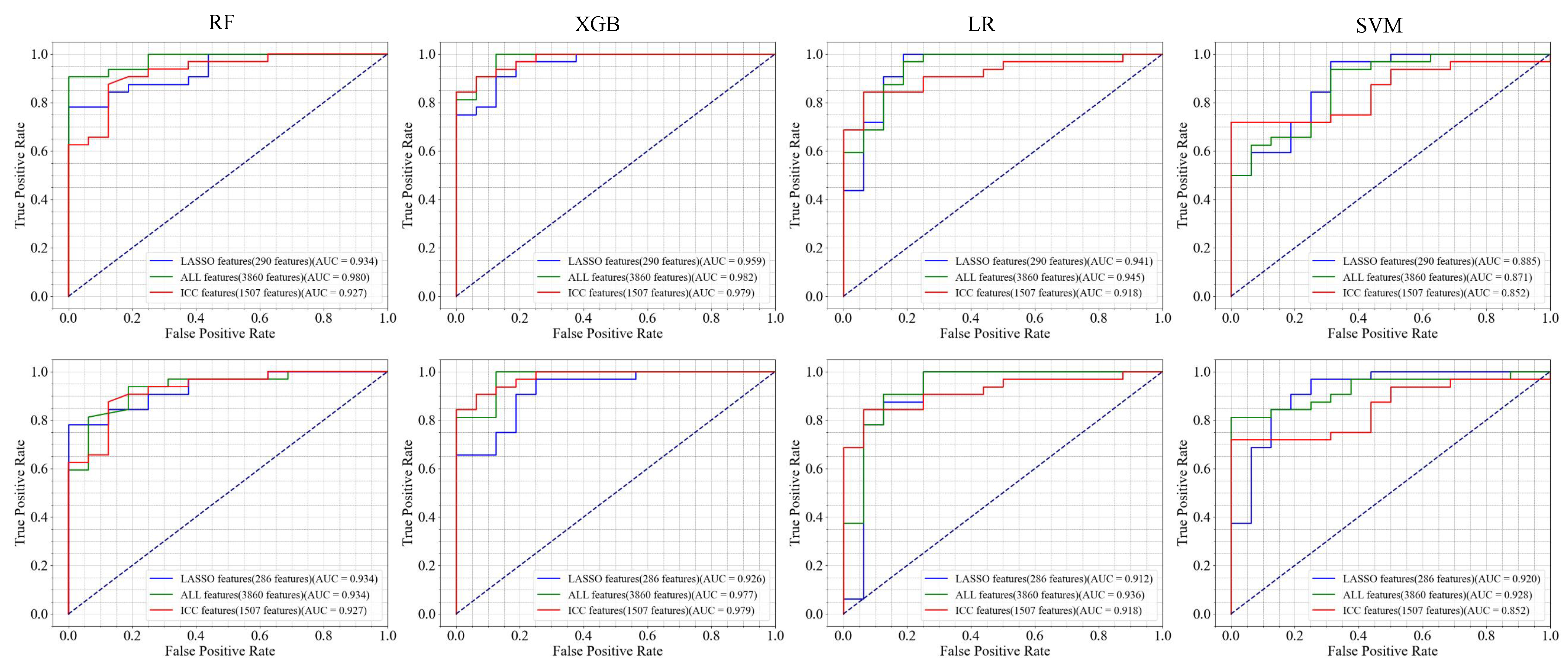
- We simulate four predictive models to classify between LGGs and GBM images using a manual and/or automatic corrected segmentation mask.
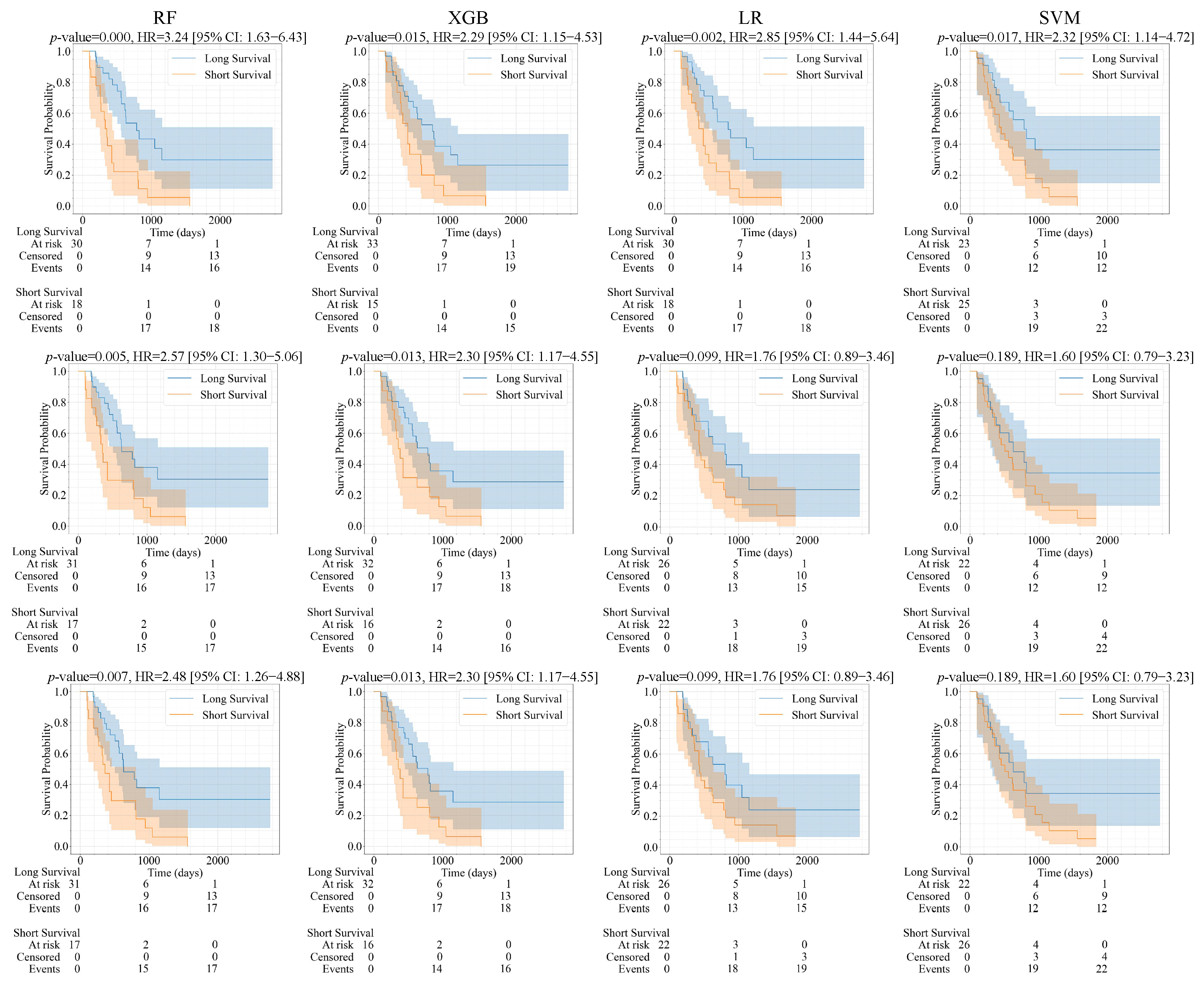
- We evaluate four predictive models in the survival analysis for the patient with brain tumor using LGG and GBM MRI images.
- We assess the impact of LASSO and ICC features in the classification of LGGs and GBM and the survival analysis.
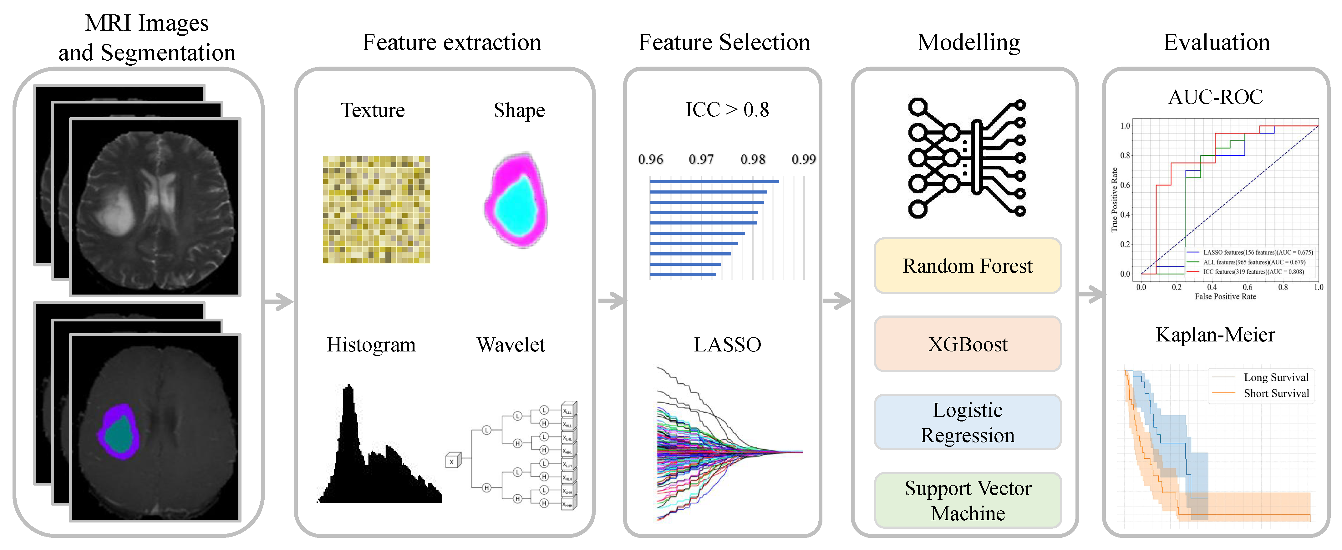
2. Method
| Algorithm 1 Pipeline of radiomics model. | |
| Require: Brain tumor MRI image I, segmentation masks and Ensure: Extracted features , trained models , performance metrics | |
| ▹ Segment image using mask ▹ Segment image using mask ▹ Extract features from the region of ▹ Extract features from the region of ▹ Apply ICC ▹ Apply LASSO regression ▹ Select stable and important features ▹ Train models using selected features ▹ Evaluate models using the test samples |
2.1. Dataset Description
2.2. Patients and Data Cleaning
2.3. Feature Extraction
2.4. Feature Selection
2.4.1. Interclass Correlation Coefficient-ICC
2.4.2. LASSO
2.5. Experimental Environment Details and Modeling
2.6. Performance Evaluation
2.7. Survival Analysis
3. Result
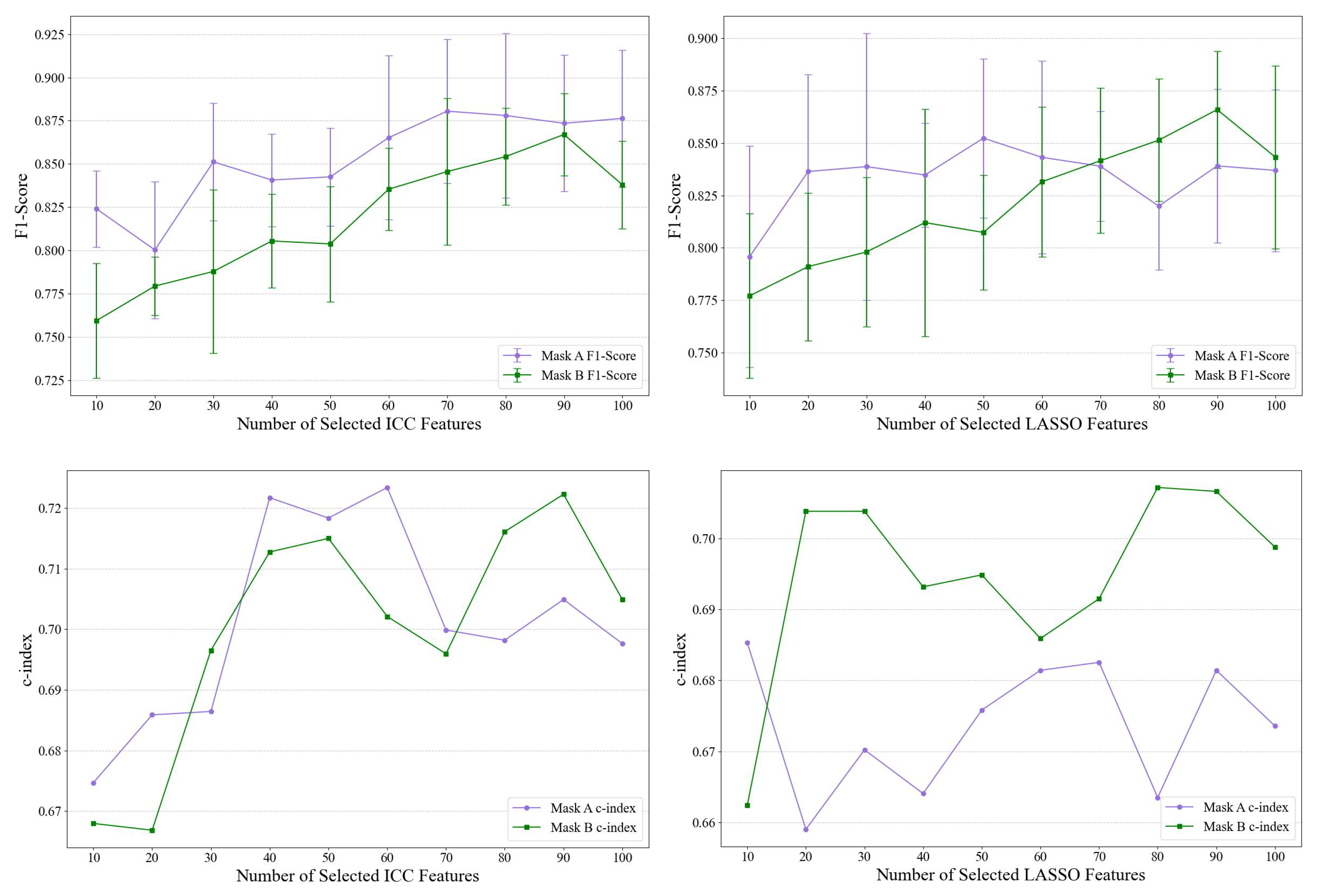
Ablation Study
4. Discussion
5. Conclusions
Author Contributions
Funding
Institutional Review Board Statement
Informed Consent Statement
Data Availability Statement
Acknowledgments
Conflicts of Interest
References
- Louis, D.N.; Perry, A.; Wesseling, P.; Brat, D.J.; Cree, I.A.; Figarella-Branger, D.; Hawkins, C.; Ng, H.K.; Pfister, S.M.; Reifenberger, G.; et al. The 2021 WHO Classification of Tumors of the Central Nervous System: A summary. Neuro-Oncology 2021, 23, 1231–1251. [Google Scholar] [CrossRef] [PubMed]
- Chaddad, A.; Daniel, P.; Zhang, M.; Rathore, S.; Sargos, P.; Desrosiers, C.; Niazi, T. Deep radiomic signature with immune cell markers predicts the survival of glioma patients. Neurocomputing 2022, 469, 366–375. [Google Scholar] [CrossRef]
- Chaddad, A.; Daniel, P.; Sabri, S.; Desrosiers, C.; Abdulkarim, B. Integration of radiomic and multi-omic analyses predicts survival of newly diagnosed IDH1 wild-type glioblastoma. Cancers 2019, 11, 1148. [Google Scholar] [CrossRef]
- Weller, M.; Wen, P.Y.; Chang, S.M.; Dirven, L.; Lim, M.; Monje, M.; Reifenberger, G. Glioma. Nat. Rev. Dis. Prim. 2024, 10, 33. [Google Scholar] [CrossRef] [PubMed]
- Chaddad, A.; Kucharczyk, M.J.; Daniel, P.; Sabri, S.; Jean-Claude, B.J.; Niazi, T.; Abdulkarim, B. Radiomics in glioblastoma: Current status and challenges facing clinical implementation. Front. Oncol. 2019, 9, 374. [Google Scholar] [CrossRef]
- Al-Zoghby, A.M.; Al-Awadly, E.M.K.; Moawad, A.; Yehia, N.; Ebada, A.I. Dual deep cnn for tumor brain classification. Diagnostics 2023, 13, 2050. [Google Scholar] [CrossRef] [PubMed]
- Bijari, S.; Sayfollahi, S.; Mardokh-Rouhani, S.; Bijari, S.; Moradian, S.; Zahiri, Z.; Rezaeijo, S.M. Radiomics and Deep Features: Robust Classification of Brain Hemorrhages and Reproducibility Analysis Using a 3D Autoencoder Neural Network. Bioengineering 2024, 11, 643. [Google Scholar] [CrossRef]
- Assegie, T.A.; Sushma, S.; Mamanazarovna, S.S. Explainable Heart Disease Diagnosis with Supervised Learning Methods. ADCAIJ Adv. Distrib. Comput. Artif. Intell. J. 2023, 12, e31228. [Google Scholar] [CrossRef]
- Tabassum, M.; Suman, A.A.; Suero Molina, E.; Pan, E.; Di Ieva, A.; Liu, S. Radiomics and Machine Learning in Brain Tumors and Their Habitat: A Systematic Review. Cancers 2023, 15, 3845. [Google Scholar] [CrossRef]
- Kumar, A.; Jha, A.K.; Agarwal, J.P.; Yadav, M.; Badhe, S.; Sahay, A.; Epari, S.; Sahu, A.; Bhattacharya, K.; Chatterjee, A.; et al. Machine-learning-based radiomics for classifying glioma grade from magnetic resonance images of the brain. J. Pers. Med. 2023, 13, 920. [Google Scholar] [CrossRef]
- Park, J.H.; Quang, L.T.; Yoon, W.; Baek, B.H.; Park, I.; Kim, S.K. Predicting Histologic Grade of Meningiomas Using a Combined Model of Radiomic and Clinical Imaging Features from Preoperative MRI. Biomedicines 2023, 11, 3268. [Google Scholar] [CrossRef] [PubMed]
- Gu, S.; Qian, J.; Yang, L.; Sun, Z.; Hu, C.; Wang, X.; Hu, S.; Xie, Y. Multiparametric MRI radiomics for the differentiation of brain glial cell hyperplasia from low-grade glioma. BMC Med. Imaging 2023, 23, 116. [Google Scholar] [CrossRef] [PubMed]
- Zhang, H.; Zhang, H.; Zhang, Y.; Zhou, B.; Wu, L.; Yang, W.; Lei, Y.; Huang, B. Multiparametric MRI-based fusion radiomics for predicting telomerase reverse transcriptase (TERT) promoter mutations and progression-free survival in glioblastoma: A multicentre study. Neuroradiology 2024, 66, 81–92. [Google Scholar] [CrossRef]
- Björkblom, B.; Wibom, C.; Eriksson, M.; Bergenheim, A.T.; Sjöberg, R.L.; Jonsson, P.; Brännström, T.; Antti, H.; Sandström, M.; Melin, B. Distinct metabolic hallmarks of WHO classified adult glioma subtypes. Neuro-Oncology 2022, 24, 1454–1468. [Google Scholar] [CrossRef] [PubMed]
- Du, P.; Liu, X.; Wu, X.; Chen, J.; Cao, A.; Geng, D. Predicting Histopathological Grading of Adult Gliomas Based On Preoperative Conventional Multimodal MRI Radiomics: A Machine Learning Model. Brain Sci. 2023, 13, 912. [Google Scholar] [CrossRef]
- Joo, B.; Ahn, S.S.; An, C.; Han, K.; Choi, D.; Kim, H.; Park, J.E.; Kim, H.S.; Lee, S.K. Fully automated radiomics-based machine learning models for multiclass classification of single brain tumors: Glioblastoma, lymphoma, and metastasis. J. Neuroradiol. 2023, 50, 388–395. [Google Scholar] [CrossRef]
- Zhu, F.Y.; Sun, Y.F.; Yin, X.P.; Wang, T.D.; Zhang, Y.; Xing, L.H.; Xue, L.Y.; Wang, J.N. Use of Radiomics Models in Preoperative Grading of Cerebral Gliomas and Comparison with Three-dimensional Arterial Spin Labelling. Clin. Oncol. 2023, 35, 726–735. [Google Scholar] [CrossRef]
- Destito, M.; Marzullo, A.; Leone, R.; Zaffino, P.; Steffanoni, S.; Erbella, F.; Calimeri, F.; Anzalone, N.; De Momi, E.; Ferreri, A.J.M.; et al. Radiomics-Based Machine Learning Model for Predicting Overall and Progression-Free Survival in Rare Cancer: A Case Study for Primary CNS Lymphoma Patients. Bioengineering 2023, 10, 285. [Google Scholar] [CrossRef]
- Hussain, S.; Haider, S.; Maqsood, S.; Damaševičius, R.; Maskeliūnas, R.; Khan, M. ETISTP: An enhanced model for brain tumor identification and survival time prediction. Diagnostics 2023, 13, 1456. [Google Scholar] [CrossRef]
- Cancer Genome Atlas Research Network. Comprehensive, integrative genomic analysis of diffuse lower-grade gliomas. New Engl. J. Med. 2015, 372, 2481–2498. [Google Scholar]
- Chow, D.; Chang, P.; Weinberg, B.D.; Bota, D.A.; Grinband, J.; Filippi, C.G. Imaging genetic heterogeneity in glioblastoma and other glial tumors: Review of current methods and future directions. Am. J. Roentgenol. 2018, 210, 30–38. [Google Scholar] [CrossRef]
- Tang, Z.; Xu, Y.; Jin, L.; Aibaidula, A.; Lu, J.; Jiao, Z.; Wu, J.; Zhang, H.; Shen, D. Deep learning of imaging phenotype and genotype for predicting overall survival time of glioblastoma patients. IEEE Trans. Med. Imaging 2020, 39, 2100–2109. [Google Scholar] [CrossRef] [PubMed]
- Chato, L.; Latifi, S. Machine learning and radiomic features to predict overall survival time for glioblastoma patients. J. Pers. Med. 2021, 11, 1336. [Google Scholar] [CrossRef] [PubMed]
- Choi, Y.S.; Ahn, S.S.; Chang, J.H.; Kang, S.G.; Kim, E.H.; Kim, S.H.; Jain, R.; Lee, S.K. Machine learning and radiomic phenotyping of lower grade gliomas: Improving survival prediction. Eur. Radiol. 2020, 30, 3834–3842. [Google Scholar] [CrossRef]
- Le, V.H.; Minh, T.N.T.; Kha, Q.H.; Le, N.Q.K. A transfer learning approach on MRI-based radiomics signature for overall survival prediction of low-grade and high-grade gliomas. Med. Biol. Eng. Comput. 2023, 61, 2699–2712. [Google Scholar] [CrossRef] [PubMed]
- Bakas, S.; Shukla, G.; Akbari, H.; Erus, G.; Sotiras, A.; Rathore, S.; Sako, C.; Min Ha, S.; Rozycki, M.; Shinohara, R.T.; et al. Overall survival prediction in glioblastoma patients using structural magnetic resonance imaging (MRI): Advanced radiomic features may compensate for lack of advanced MRI modalities. J. Med. Imaging 2020, 7, 031505. [Google Scholar] [CrossRef]
- Hermoza, R.; Maicas, G.; Nascimento, J.C.; Carneiro, G. Post-hoc overall survival time prediction from brain MRI. In Proceedings of the 2021 IEEE 18th International Symposium on Biomedical Imaging (ISBI), Nice, France, 13–16 April 2021; IEEE: Piscataway, NJ, USA, 2021; pp. 1476–1480. [Google Scholar]
- Soltani, M.; Bonakdar, A.; Shakourifar, N.; Babaei, R.; Raahemifar, K. Efficacy of location-based features for survival prediction of patients with glioblastoma depending on resection status. Front. Oncol. 2021, 11, 661123. [Google Scholar] [CrossRef]
- Trinh, D.L.; Kim, S.H.; Yang, H.J.; Lee, G.S. The Efficacy of Shape Radiomics and Deep Features for Glioblastoma Survival Prediction by Deep Learning. Electronics 2022, 11, 1038. [Google Scholar] [CrossRef]
- Zhu, J.; Ye, J.; Dong, L.; Ma, X.; Tang, N.; Xu, P.; Jin, W.; Li, R.; Yang, G.; Lai, X. Non-invasive prediction of overall survival time for glioblastoma multiforme patients based on multimodal MRI radiomics. Int. J. Imaging Syst. Technol. 2023, 33, 1261–1274. [Google Scholar] [CrossRef]
- Bakas, S.; Akbari, H.; Sotiras, A.; Bilello, M.; Rozycki, M.; Kirby, J.S.; Freymann, J.B.; Farahani, K.; Davatzikos, C. Advancing the cancer genome atlas glioma MRI collections with expert segmentation labels and radiomic features. Sci. Data 2017, 4, 170117. [Google Scholar] [CrossRef]
- Li, Y.; Ammari, S.; Lawrance, L.; Quillent, A.; Assi, T.; Lassau, N.; Chouzenoux, E. Radiomics-based method for predicting the glioma subtype as defined by tumor grade, IDH mutation, and 1p/19q codeletion. Cancers 2022, 14, 1778. [Google Scholar] [CrossRef] [PubMed]
- van Griethuysen, J.J.M.; Fedorov, A.; Parmar, C.; Hosny, A.; Aucoin, N.; Narayan, V.; Beets-Tan, R.G.H.; Fillion-Robin, J.C.; Pieper, S.; Aerts, H.J.W.L. Computational Radiomics System to Decode the Radiographic Phenotype. Front. Oncol. 2017, 4, 303. [Google Scholar] [CrossRef]
- Chaddad, A.; Daniel, P.; Desrosiers, C.; Toews, M.; Abdulkarim, B. Novel radiomic features based on joint intensity matrices for predicting glioblastoma patient survival time. IEEE J. Biomed. Health Inform. 2018, 23, 795–804. [Google Scholar] [CrossRef] [PubMed]
- Chaddad, A.; Wang, Y.; Feng, J. Radiomics for a Comprehensive Assessment of Glioblastoma Multiforme. In Proceedings of the 2023 IEEE International Conference on E-Health Networking, Application and Services (Healthcom), Chongqing, China, 15–17 December 2023; pp. 253–258. [Google Scholar] [CrossRef]
- Koo, T.K.; Li, M.Y. A guideline of selecting and reporting intraclass correlation coefficients for reliability research. J. Chiropr. Med. 2016, 15, 155–163. [Google Scholar] [CrossRef]
- Tibshirani, R. Regression shrinkage and selection via the lasso. J. R. Stat. Soc. Ser. B Methodol. 1996, 58, 267–288. [Google Scholar] [CrossRef]
- Vickers, A.J.; Elkin, E.B. Decision curve analysis: A novel method for evaluating prediction models. Med. Decis. Mak. 2006, 26, 565–574. [Google Scholar] [CrossRef]
- Chaddad, A.; Hassan, L.; Katib, Y. A texture-based method for predicting molecular markers and survival outcome in lower grade glioma. Appl. Intell. 2023, 53, 24724–24738. [Google Scholar] [CrossRef]


| GBM | |
|---|---|
| Number of patients | 97 |
| Number of segments (lesions) | 194 |
| Age (years) | |
| Median (Range) | 56.5 (18–84) |
| Gender | |
| Male | 58 |
| Female | 38 |
| Unknown | 1 |
| Os.time(days) | |
| Median (Range) | 424.5 (5–2768) |
| LGG | |
| Number of patients | 62 |
| Number of segments (lesions) | 124 |
| Age (years) | |
| Median (Range) | 43.5 (20–74) |
| Gender | |
| Male | 26 |
| Female | 36 |
| Os.time(days) | |
| Median (Range) | 788 (3–4752) |
| Feature (A/B) | Model | Accuracy | Sensitivity | Specificity | Precision | F-Score |
|---|---|---|---|---|---|---|
| LASSO features (290/286 features) | RF | 85.42/83.33 | 87.50/78.13 | 81.25/93.75 | 90.32/96.15 | 88.89/86.21 |
| SVM | 89.58/87.50 | 93.75/90.63 | 81.25/81.25 | 90.91/90.63 | 88.52/82.76 | |
| LR | 89.58/87.50 | 93.75/90.63 | 81.25/81.25 | 90.91/90.63 | 92.31/90.63 | |
| XGB | 85.42/79.17 | 84.38/75.00 | 87.50/87.50 | 93.10/92.30 | 88.52/82.76 | |
| ALL features (3860/3860 features) | RF | 91.67/85.42 | 87.50/81.25 | 100.00/93.75 | 100.00/96.30 | 93.33/88.14 |
| SVM | 87.50/89.58 | 90.63/90.63 | 81.25/87.50 | 90.63/93.55 | 90.63/92.06 | |
| LR | 87.50/89.58 | 90.63/90.63 | 81.25/87.50 | 86.67/92.86 | 90.63/93.55 | |
| XGB | 91.67/83.33 | 93.75/75.00 | 87.50/100 | 93.75/100 | 93.75/85.71 | |
| ICC features (1507/1507 features) | RF | 75.00/75.00 | 68.75/68.75 | 87.50/87.50 | 91.67/91.67 | 78.57/78.57 |
| SVM | 77.08/83.33 | 71.88/90.63 | 87.50/68.75 | 92.00/85.29 | 80.70/87.88 | |
| LR | 83.33/83.33 | 90.63/90.63 | 68.75/68.75 | 85.29/85.29 | 87.88/87.88 | |
| XGB | 83.33/83.33 | 75.00/75.00 | 100.00/100.00 | 100.00/100.00 | 85.71/85.71 | |
| Combined ICC and LASSO (1715/1709 features) | RF | 89.58/81.25 | 84.38/75.00 | 100.00/93.75 | 100.00/96.00 | 91.53/84.21 |
| SVM | 85.42/85.42 | 84.38/78.13 | 87.50/100.00 | 93.10/100.00 | 88.52/87. 72 | |
| LR | 85.42/85.42 | 84.38/78.13 | 87.50/100.00 | 93.10/100.00 | 88.52/87.72 | |
| XGB | 89.58/83.33 | 90.63/78.13 | 87.50/93.75 | 93.55/96.15 | 92.06/86.21 |
| Feature (A/B) | Model | Accuracy | Sensitivity | Specificity | Precision | F-Score |
|---|---|---|---|---|---|---|
| RF | 83.08 ± 7.23/81.13 ± 3.43 | 86.79 ± 7.98/89.79 ± 4.36 | 77.44 ± 9.42/67.82 ± 8.15 | 85.87 ± 5.46/81.52 ± 3.82 | 86.19 ± 5.95/85.32 ± 2.47 | |
| LASSO features | SVM | 77.98 ± 4.43/77.98 ± 6.56 | 85.68 ± 5.71/86.68 ± 3.76 | 66.03 ± 4.01/64.36 ± 13.85 | 79.79 ± 1.92/79.64 ± 6.44 | 82.58 ± 3.48/82.90 ± 4.45 |
| (290/286 features) | LR | 77.98 ± 1.99/83.63 ± 3.73 | 87.68 ± 3.85/88.68 ± 3.81 | 62.82 ± 8.67/76.03 ± 9.56 | 78.94 ± 3.25/85.47 ± 5.47 | 82.94 ± 1.12/86.88 ± 2.83 |
| XGB | 83.71 ± 9.31/82.98 ± 6.84 | 88.84 ± 8.56/90.84 ± 7.48 | 75.77 ± 11.65/70.77 ± 8.76 | 85.23 ± 6.94/83.07 ± 4.51 | 86.95 ± 7.43/86.69 ± 5.30 | |
| RF | 87.42 ± 1.98/86.79 ± 4.14 | 91.74 ± 2.57/91.74 ± 4.20 | 80.51 ± 6.95/78.85 ± 6.77 | 88.31 ± 2.86/87.35 ± 3.76 | 89.93 ± 1.30/89.45 ± 3.45 | |
| ALL features | SVM | 85.52 ± 4.27/80.54 ± 4.89 | 88.57 ± 4.06/84.47 ± 4.84 | 80.51 ± 10.73/74.23 ± 9.05 | 88.27 ± 6.68/83.91 ± 5.19 | 88.22 ± 3.40/84.09 ± 4.11 |
| (3860/3860 features) | LR | 84.90 ± 3.67/84.29 ± 2.71 | 86.47 ± 6.44/87.63 ± 2.49 | 82.18 ± 3.64/79.10 ± 3.52 | 88.39 ± 1.92/86.74 ± 2.47 | 87.31 ± 3.68/87.17 ± 2.31 |
| XGB | 86.81 ± 2.24/88.69 ± 4.21 | 92.74 ± 2.67/91.74 ± 7.13 | 77.31 ± 6.46/83.85 ± 5.31 | 86.69 ± 2.77/89.92 ± 2.87 | 89.56 ± 1.76/90.66 ± 3.99 | |
| RF | 86.77 ± 4.21/86.79 ± 3.05 | 91.68 ± 4.29/90.68 ± 6.16 | 79.10 ± 6.34/80.51 ± 4.53 | 87.26 ± 3.94/88.06 ± 1.79 | 89.37 ± 3.60/89.22 ± 3.07 | |
| ICC features | SVM | 85.51 ± 3.90/84.88 ± 3.77 | 85.42 ± 7.12/92.68 ± 7.89 | 85.26 ± 6.51/72.56 ± 12.54 | 90.43 ± 3.49/84.80 ± 5.99 | 87.63 ± 3.80/88.12 ± 3.10 |
| (1507/1507 features) | LR | 84.23 ± 4.62/86.11 ± 4.92 | 84.37 ± 7.59/87.53 ± 5.48 | 83.72 ± 5.49/83.59 ± 9.37 | 89.21 ± 3.28/89.73 ± 5.17 | 86.52 ± 4.41/88.47 ± 4.01 |
| XGB | 88.04 ± 1.30/87.44 ± 3.37 | 93.79 ± 2.16/90.74 ± 7.64 | 78.97 ± 4.16/82.31 ± 5.94 | 87.55 ± 2.02/89.05 ± 3.17 | 90.53 ± 1.12/89.63 ± 3.42 | |
| RF | 88.02 ± 3.75/87.42 ± 1.98 | 92.74 ± 2.67/91.74 ± 5.36 | 80.51 ± 8.72/80.26 ± 11.57 | 88.42 ± 4.30/88.76 ± 5.26 | 90.47 ± 2.83/89.93 ± 1.24 | |
| Combined ICC and LASSO | SVM | 86.15 ± 2.58/85.52 ± 1.62 | 87.53 ± 5.48/89.63 ± 7.48 | 83.46 ± 11.88/78.59 ± 13.79 | 90.27 ± 6.22/87.93 ± 6.03 | 88.54 ± 2.02/88.27 ± 1.41 |
| (1715/1709 features) | LR | 87.44 ± 3.37/86.79 ± 3.63 | 87.53 ± 7.96/88.58 ± 7.80 | 86.92 ± 4.40/83.59 ± 10.75 | 91.59 ± 1.77/90.17 ± 5.02 | 89.24 ± 3.73/88.98 ± 3.60 |
| XGB | 86.17 ± 1.47/86.81 ± 3.58 | 91.79 ± 3.98/90.84 ± 6.62 | 77.44 ± 3.07/80.77 ± 7.83 | 86.45 ± 1.57/88.29 ± 3.08 | 88.97 ± 1.47/89.30 ± 3.08 |
| Feature (A/B) | Model | p-Value | HR | CI | C-Index | Brier Score |
|---|---|---|---|---|---|---|
| RF | 0.018/0.007 | 2.21/2.48 | 1.13–4.35/1.26–4.88 | 0.689/0.690 | 0.111/0.121 | |
| LASSO features | SVM | 0.002/0.189 | 3.56/1.60 | 1.54–8.27/0.79–3.23 | 0.609/0.567 | 0.142/0.185 |
| (1417/3857 features) | LR | 0.062/0.099 | 1.88/1.76 | 0.96–3.71/0.89–3.46 | 0.636/0.623 | 0.211/0.144 |
| XGB | 0.002/0.013 | 2.85/2.30 | 1.44–5.64/1.17–4.55 | 0.664/0.689 | 0.111/0.079 | |
| RF | 0.012/0.005 | 2.33/2.57 | 1.18–4.59/1.30–5.06 | 0.681/0.718 | 0.108/0.119 | |
| ALL features | SVM | 0.002/0.189 | 3.56/1.60 | 1.54–8.27/0.79–3.23 | 0.610/0.567 | 0.145/0.184 |
| (3861/3861 features) | LR | 0.062/0.099 | 1.88/1.76 | 0.96–3.71/0.89–3.46 | 0.634/0.612 | 0.214/0.137 |
| XGB | 0.037/0.013 | 2.08/2.30 | 1.03–4.18/1.17–4.55 | 0.652/0.689 | 0.131/0.080 | |
| RF | 0.0003/0.0003 | 3.24/3.24 | 1.63–4.43/1.63–4.43 | 0.719/0.719 | 0.113/0.113 | |
| ICC features | SVM | 0.011/0.017 | 2.53/2.32 | 1.20–5.30/1.14–4.72 | 0.592/0.592 | 0.200/0.189 |
| (1508/1508 features) | LR | 0.002/0.002 | 2.85/2.85 | 1.44–5.64/1.44–5.64 | 0.695/0.695 | 0.173/0.173 |
| XGB | 0.015/0.015 | 2.29/2.29 | 1.15–4.53/1.15–4.53 | 0.669/0.669 | 0.085/0.085 | |
| RF | 0.002/0.003 | 2.83/2.67 | 1.43–5.59/1.35–5.26 | 0.701/0.711 | 0.105/0.119 | |
| Combined ICC and LASSO | SVM | 0.002/0.189 | 3.56/1.60 | 1.54–8.27/0.79–3.23 | 0.610/0.567 | 0.143/0.181 |
| (2537/3858 features) | LR | 0.062/0.140 | 1.88/1.66 | 0.96–3.71/0.84–3.27 | 0.634/0.623 | 0.212/0.164 |
| XGB | 0.005/0.034 | 2.57/2.06 | 1.29–5.11/1.04–4.08 | 0.651/0.669 | 0.132/0.073 |
Disclaimer/Publisher’s Note: The statements, opinions and data contained in all publications are solely those of the individual author(s) and contributor(s) and not of MDPI and/or the editor(s). MDPI and/or the editor(s) disclaim responsibility for any injury to people or property resulting from any ideas, methods, instructions or products referred to in the content. |
© 2025 by the authors. Licensee MDPI, Basel, Switzerland. This article is an open access article distributed under the terms and conditions of the Creative Commons Attribution (CC BY) license (https://creativecommons.org/licenses/by/4.0/).
Share and Cite
Chaddad, A.; Jia, P.; Hu, Y.; Katib, Y.; Kateb, R.; Daqqaq, T.S. A Radiomic Model for Gliomas Grade and Patient Survival Prediction. Bioengineering 2025, 12, 450. https://doi.org/10.3390/bioengineering12050450
Chaddad A, Jia P, Hu Y, Katib Y, Kateb R, Daqqaq TS. A Radiomic Model for Gliomas Grade and Patient Survival Prediction. Bioengineering. 2025; 12(5):450. https://doi.org/10.3390/bioengineering12050450
Chicago/Turabian StyleChaddad, Ahmad, Pingyue Jia, Yan Hu, Yousef Katib, Reem Kateb, and Tareef Sahal Daqqaq. 2025. "A Radiomic Model for Gliomas Grade and Patient Survival Prediction" Bioengineering 12, no. 5: 450. https://doi.org/10.3390/bioengineering12050450
APA StyleChaddad, A., Jia, P., Hu, Y., Katib, Y., Kateb, R., & Daqqaq, T. S. (2025). A Radiomic Model for Gliomas Grade and Patient Survival Prediction. Bioengineering, 12(5), 450. https://doi.org/10.3390/bioengineering12050450