
Improved Confidence-Interval Estimations Using Uncertainty Measure and Weighted Feature Decisions for Cuff-Less Blood-Pressure Measurements


Abstract
1. Introduction
- We develop a method to combine dual-step preprocessing and multiple feature extraction (DPFE) and WFD based on GPR to improve the reliability of cuff-less BP estimates and individual uncertainty estimates.
- The proposed method measures uncertainties such as CIs and expanded uncertainty for cuff-less BP measurement.
- The proposed method provides more accurate prediction performance and uncertainty by providing lower standard deviation (SD), mean absolute error, and CI. Therefore, it can help estimate BP and CI for clinical practice or diagnostic purposes.
2. Data Collection
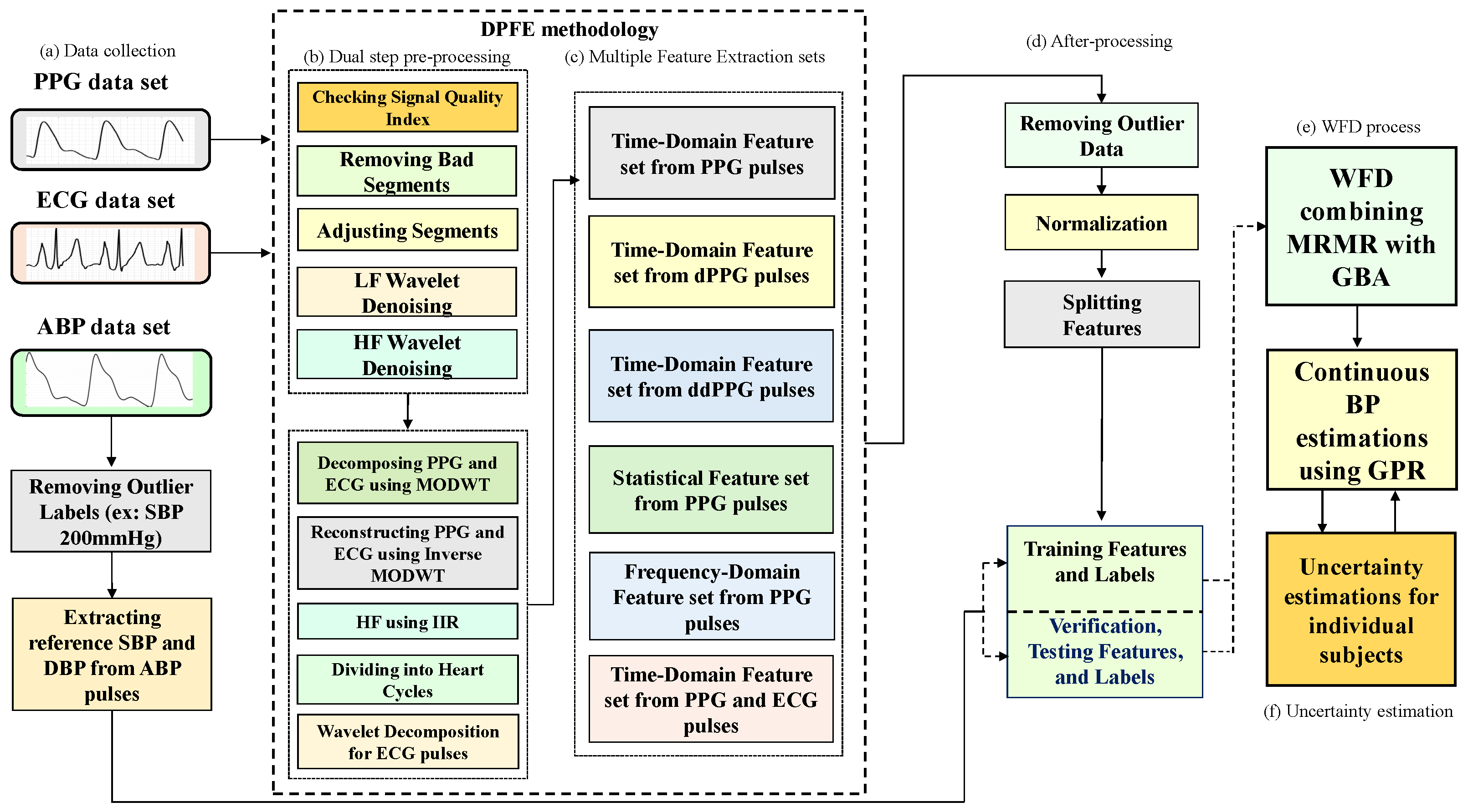
3. Methods
3.1. Dual-Stage Preprocessing for Features Extraction
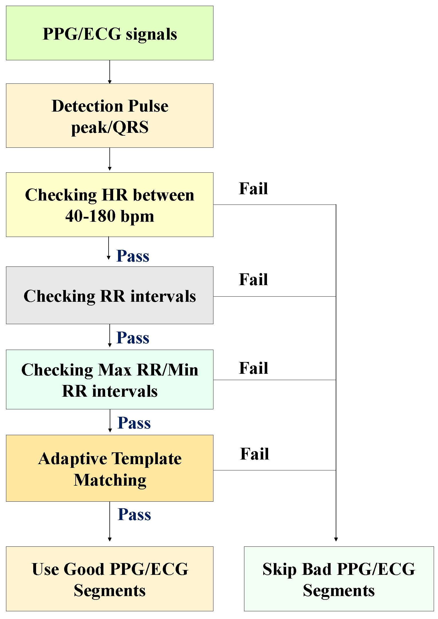
3.2. Signal Quality Index (SQI)
- We compute the median beat interval using all detected R-peaks/PPG pulse peaks in each PPG/ECG sample.
- We leave no stone unturned in our analysis. Individual PPG pulses and QRS complexes are extracted by taking a window centered around each detected PPG pulse peak and R-peak, with the window width being the median beat interval.
- We obtain the average PPG pulse template by calculating the average of all PPG pulses in the sample. Then, we compute the correlation coefficient of each PPG pulse and the average PPG pulse template. We also acquired the average QRS template by taking the mean of all QRS complexes in the sample. Then, we calculate the correlation coefficient of individual QRS complexes with the average QRS template.
- The average correlation coefficient is finally obtained by averaging all correlation coefficients of all PPG and ECG samples. Examples of QRS complex and PPG pulses and generated templates from morphologically regular and irregular signal samples are shown in Figure 2, respectively.
3.3. Review of Feature Extraction
3.4. MRMR
| Algorithm 1 MRMR(, ) |
|
3.5. GBA
| Algorithm 2 Weighted feature decision (WFD) |
|
4. GPR
5. Uncertainty Estimation for Individual Subject
5.1. Measurement Uncertainty
5.2. CI Estimation Using Bootstrap for Individual Subject
5.3. CL Estimation Using Monte Carlo for Individual Subject
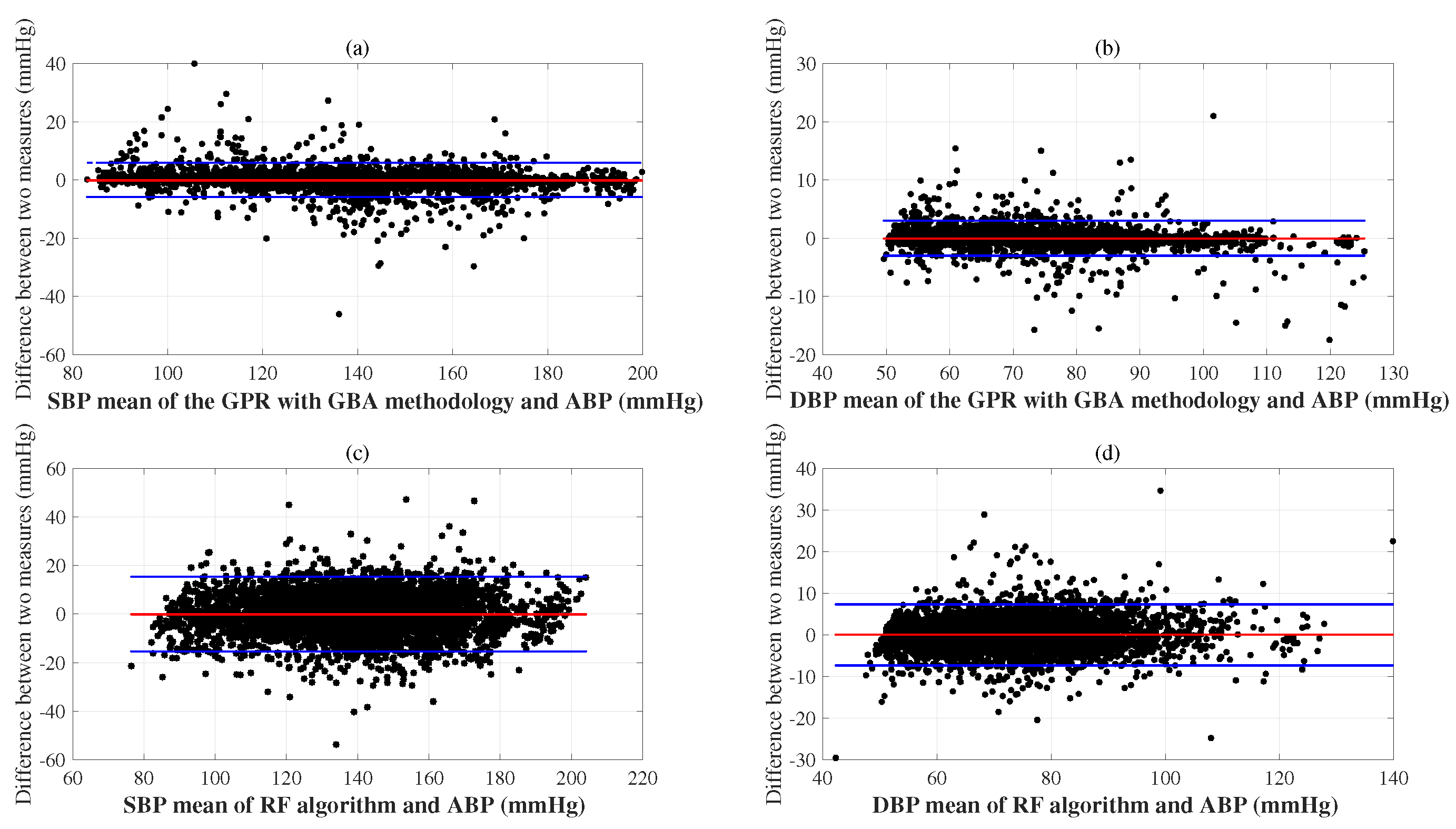
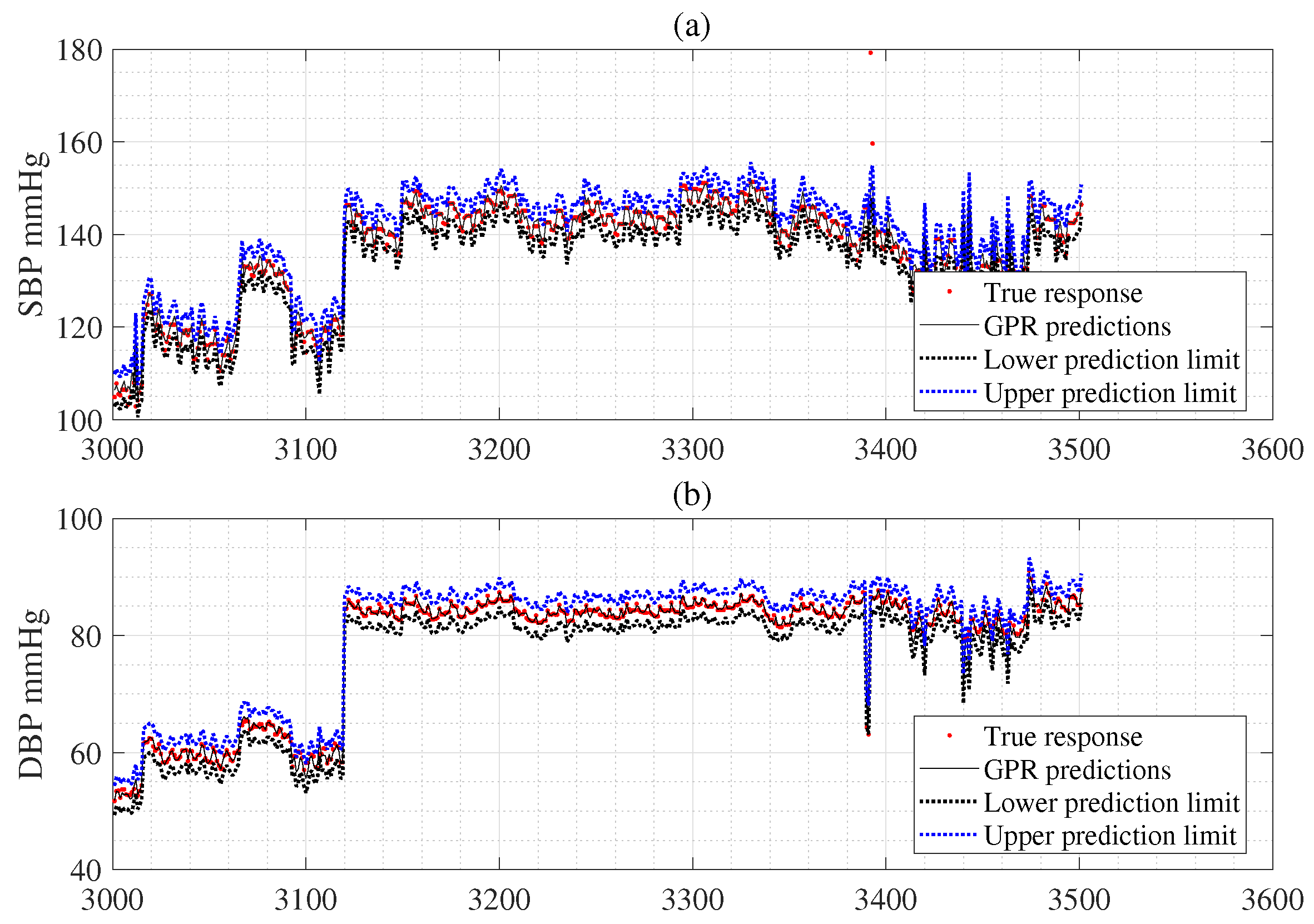
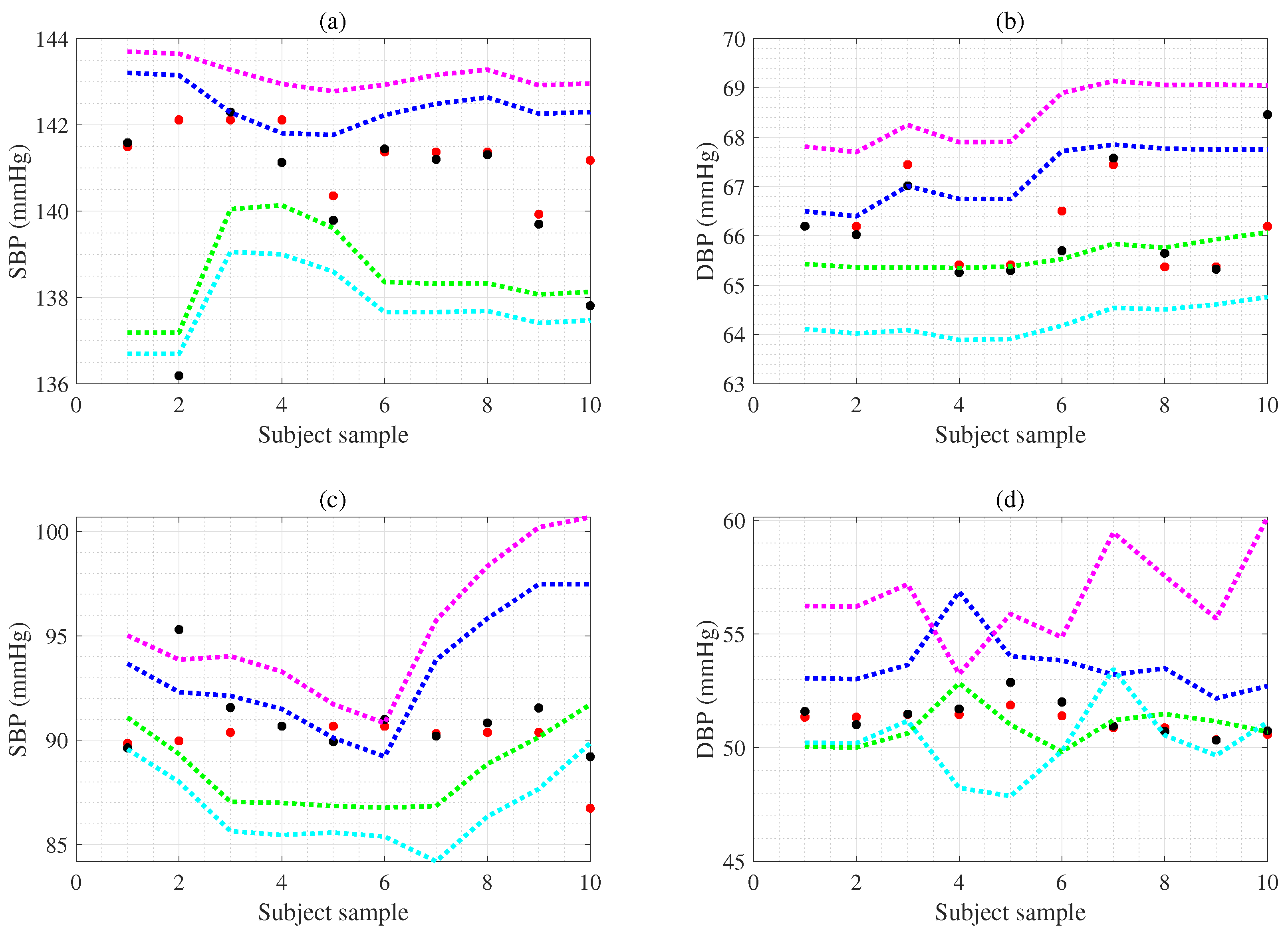
6. Experimental Results

| Method Combined (mmHg) | SVM [38] | NN [10] | DNN [45] | RTree [39] | RF [42] | GPR [15] | GPR [15] | |||||||
|---|---|---|---|---|---|---|---|---|---|---|---|---|---|---|
| SBP | DBP | SBP | DBP | SBP | DBP | SBP | DBP | SBP | DBP | SBP | DBP | SBP | DBP | |
| DPFE | DPFE | DPFE | DPFE | DPFE | DPFE | DPFE&WFD | ||||||||
| MAE | 1.87 | 0.94 | 8.75 | 4.50 | 6.09 | 2.64 | 2.92 | 1.47 | 3.14 | 1.49 | 1.54 | 0.73 | 1.46 | 0.69 |
| SD | 0.08 | 0.02 | 0.23 | 0.06 | 0.21 | 0.08 | 0.00 | 0.00 | 0.02 | 0.01 | 0.01 | 0.01 | 0.03 | 0.01 |
| Method | Dataset | SBP (mmHg) | DBP (mmHg) | Published | ||
|---|---|---|---|---|---|---|
| MAE | SD | MAE | SD | |||
| SVM [17] | MIMIC-II (910 samples) | 8.54 | 10.90 | 4.34 | 5.80 | 2017 |
| NN [16] | MIMIC-II (2000 samples) | 4.24 | 5.05 | 4.81 | 6.37 | 2021 |
| RF [50] | Private DB (90 samples) | 7.36 | 7.15 | 5.43 | 5.30 | 2024 |
| DNN (MLPLSTM) [51] | MIMIC-II (3000 samples) | 4.39 | 6.43 | 2.54 | 3.76 | 2022 |
| DNN (RES-FRN) [52] | MIMIC III (833 subjects) | 5.59 | 5.78 | 3.35 | 3.80 | 2023 |
| DNN (CNN-LSTM) [53] | MIMIC III (431 subjects) | 4.15 | 5.83 | 2.33 | 3.16 | 2024 |
| DNN (CNN-Transformer) [54] | Aurora-BP DB (1125 subjects) | 5.25 | n/a | 6.10 | n/a | 2024 |
| DNN (Transformer+encoders) [8] | MIMIC III (1000 subjects) | 3.91 | 5.65 | 2.29 | 3.01 | 2025 |
| DNN (CNN+Transformer) [55] | MIMIC III (808 subjects) | 4.44 | 5.98 | 2.36 | 3.22 | 2025 |
| GPR DPFE & WFD | MIMIC-II (3000 subjects, 59,097 samples) | 1.46 | 0.03 | 0.69 | 0.01 | |
7. Discussion
Limitations and Further Discussion
8. Conclusions
Author Contributions
Funding
Institutional Review Board Statement
Informed Consent Statement
Data Availability Statement
Acknowledgments
Conflicts of Interest
Abbreviations
| BP | Blood pressure |
| WFS | Weighted feature selection |
| DPFE | Dual-stage preprocessing and feature extraction |
| GBA | Gradient boosting algorithm |
| WHO | World Health Organization |
| NN | Neural network |
| PPG | Photoplethysmography |
| CI | Confidence Interval |
| LSTM | Long short-term memory |
| ECG | Electrocardiogram |
| CNN | Convolutional neural network |
| SVM | Support vector machine |
| PTT | Pulse transfer time |
| PAT | Pulse arrival time |
| NCA | Neighbor component analysis |
| RNCA | Robust neighbor component analysis |
| MRMR | Minimum redundancy maximum relevance |
| GPR | Gaussian process regression |
| DNN | Deep neural network |
| MIMIC | Multiparameter intelligent monitoring in intensive care |
| SBP | Systolic blood pressure |
| DBP | Diastolic blood pressure |
| db8 | Daubechies 8 wavelet |
| MODWT | Maximum overlap discrete wavelet transform |
| PIR | Pulse intensity ratio |
| ST | Systolic time |
| DT | Diastolic time |
| CT | Cycle time |
| DA | Diastolic area |
| SA | Systolic area |
| SW | Width-dependent parameters of the systolic areas |
| DW | Width-dependent parameters of the diastolic areas |
| MSE | Mean squared error |
| MAE | Mean absolute error |
| SD | Standard deviation |
| RF | Random forests |
| RTree | Regression tree |
| BIDMC | Beth Israel Deaconess Medical Center |
| MAE | Mean absolute error |
| CMAE | cumulative MAE |
| ME | Mean error |
| AAMI | Advancement of medical instrumentation |
| BHS | British Hypertension Society |
References
- Tomitani, N.; Kanegae, H.; Kario, K. The effect of psychological stress and physical activity on ambulatory blood pressure variability detected by a multisensor ambulatory blood pressure monitoring device. Hypertens. Res. 2023, 46, 916–921. [Google Scholar] [CrossRef] [PubMed]
- Schwartz, J.E.; Warren, K.; Pickering, T.G. Mood, location and physical position as predictors of ambulatory blood pressure and heart rate: Application of a multi-level random effects model. Ann. Behav. Med. 1994, 16, 210–220. [Google Scholar] [CrossRef]
- Leito, I.; Jalukse, L.; Helm, I. Estimation of Measurement Uncertainty in Chemical Analysis (Analytical Chemistry) Course; University of Tartu: Tartu, Estonia, 2018. [Google Scholar]
- Lee, S.; Dajani, H.R.; Rajan, S.; Lee, G.; Groza, V.Z. Uncertainty in blood pressure measurement estimated using ensemble-based recursive methodology. Sensors 2020, 20, 2108. [Google Scholar] [CrossRef]
- Parvis, M.; Vallan, A. Medical measurements and uncertainties. IEEE Instrum. Meas. Mag. 2002, 5, 12–17. [Google Scholar] [CrossRef]
- Lee, S.; Bolic, M.; Groza, V.Z.; Dajani, H.R.; Rajan, S. Confidence interval estimation for oscillometric blood pressure measurements using bootstrap approaches. IEEE Trans. Instrum. Meas. 2011, 60, 3405–3415. [Google Scholar] [CrossRef]
- Lee, S.; Joshi, G.P.; Son, C.H.; Lee, G. Combining Gaussian Process with Hybrid Optimal Feature Decision in Cuffless Blood Pressure Estimation. Diagnostics 2023, 13, 736. [Google Scholar] [CrossRef]
- Huang, Z.; Shao, J.; Zhou, P.; Liu, B.; Zhu, J.; Fang, D. Continuous blood pressure monitoring based on transformer encoders and stacked attention gated recurrent units. Biomed. Signal Process. Control 2025, 99, 106860. [Google Scholar] [CrossRef]
- Sideris, C.; Kalantarian, H.; Nemati, E.; Sarrafzadeh, M. Building continuous arterial blood pressure prediction models using recurrent networks. In Proceedings of the 2016 IEEE International Conference on Smart Computing (SMARTCOMP), St Louis, MO, USA, 18–20 May 2016; pp. 1–5. [Google Scholar]
- Qiu, Z.; Chen, D.; Ling, B.W.K.; Liu, Q.; Li, W. Joint regression network and window function-based piecewise neural network for cuffless continuous blood pressure estimation only using single photoplethesmogram. IEEE Trans. Consum. Electron. 2022, 68, 236–260. [Google Scholar] [CrossRef]
- Guo, C.Y.; Chang, C.C.; Wang, K.J.; Hsieh, T.L. Assessment of a calibration-free method of cuffless blood pressure measurement: A pilot study. IEEE J. Transl. Eng. Health Med. 2022, 11, 318–329. [Google Scholar] [CrossRef]
- Yang, W.; Wang, K.; Zuo, W. Neighborhood component feature selection for high-dimensional data. J. Comput. 2012, 7, 161–168. [Google Scholar] [CrossRef]
- Akinpelu, S.; Viriri, S. Robust feature selection-based speech emotion classification using deep transfer learning. Appl. Sci. 2022, 12, 8265. [Google Scholar] [CrossRef]
- Ding, C.; Peng, H. Minimum redundancy feature selection from microarray gene expression data. J. Bioinform. Comput. Biol. 2005, 3, 185–205. [Google Scholar] [CrossRef]
- Williams, C.K.; Rasmussen, C.E. Gaussian Processes for Machine Learning; MIT Press: Cambridge, MA, USA, 2006; Volume 2. [Google Scholar]
- Maher, N.; Elsheikh, G.; Anis, W.; Emara, T. Enhancement of blood pressure estimation method via machine learning. Alex. Eng. J. 2021, 60, 5779–5796. [Google Scholar] [CrossRef]
- Liu, M.; Po, L.M.; Fu, H. Cuffless blood pressure estimation based on photoplethysmography signal and its second derivative. Int. J. Comput. Theory Eng. 2017, 9, 202. [Google Scholar] [CrossRef]
- Nandi, P.; Rao, M. A novel cnn-lstm model based non-invasive cuff-less blood pressure estimation system. In Proceedings of the 2022 44th Annual International Conference of the IEEE Engineering in Medicine & Biology Society (EMBC), Glasgow, UK, 11–15 July 2022; pp. 832–836. [Google Scholar]
- Efron, B.; Tibshirani, R. Bootstrap methods for standard errors, confidence intervals, and other measures of statistical accuracy. Stat. Sci. 1986, 1, 54–75. [Google Scholar] [CrossRef]
- BIPM; ISO; IUPAC; IUPAP; OIML. Guide to the Expression of Uncertainty in Measurement—Part 6: Developing and Using Measurement Models; JCGM/WG 1: Sevres, France, 2020. [Google Scholar]
- Goldberger, A.L.; Amaral, L.A.; Glass, L.; Hausdorff, J.M.; Ivanov, P.C.; Mark, R.G.; Mietus, J.E.; Moody, G.B.; Peng, C.K.; Stanley, H.E. PhysioBank, PhysioToolkit, and PhysioNet: Components of a new research resource for complex physiologic signals. Circulation 2000, 101, e215–e220. [Google Scholar] [CrossRef]
- Fuadah, Y.N.; Lim, K.M. Classification of blood pressure levels based on photoplethysmogram and electrocardiogram signals with a concatenated convolutional neural network. Diagnostics 2022, 12, 2886. [Google Scholar] [CrossRef] [PubMed]
- Whelton, P.K.; Carey, R.M.; Mancia, G.; Kreutz, R.; Bundy, J.D.; Williams, B. Harmonization of the American College of Cardiology/American Heart Association and European Society of Cardiology/European Society of Hypertension blood pressure/hypertension guidelines: Comparisons, reflections, and recommendations. Eur. Heart J. 2022, 43, 3302–3311. [Google Scholar] [CrossRef]
- Reboussin, D.M.; Allen, N.B.; Griswold, M.E.; Guallar, E.; Hong, Y.; Lackland, D.T.; Miller, E.P.R., III; Polonsky, T.; Thompson-Paul, A.M.; Vupputuri, S. Systematic review for the 2017 ACC/AHA/AAPA/ABC/ACPM/AGS/APhA/ASH/ASPC/NMA/PCNA guideline for the prevention, detection, evaluation, and management of high blood pressure in adults: A report of the American College of Cardiology/American Heart Association Task Force on Clinical Practice Guidelines. Hypertension 2018, 71, e116–e135. [Google Scholar]
- Aronow, W.S. Treatment of hypertensive emergencies. Ann. Transl. Med. 2017, 5, S5. [Google Scholar] [CrossRef] [PubMed]
- Nagai, S.; Anzai, D.; Wang, J. Motion artefact removals for wearable ECG using stationary wavelet transform. Healthc. Technol. Lett. 2017, 4, 138–141. [Google Scholar] [CrossRef]
- Gunasekaran, K.; Kumar, V.A. Artifact removal from ECG signals using online recursive independent component analysis. J. Comput. Math. Data Sci. 2024, 13, 100102. [Google Scholar] [CrossRef]
- Ahmed, R.; Mehmood, A.; Rahman, M.M.U.; Dobre, O.A. A Deep Learning and Fast Wavelet Transform-Based Hybrid Approach for Denoising of PPG Signals. IEEE Sens. Lett. 2023, 7, 6003504. [Google Scholar] [CrossRef]
- Kachuee, M.; Kiani, M.M.; Mohammadzade, H.; Shabany, M. Cuffless blood pressure estimation algorithms for continuous health-care monitoring. IEEE Trans. Biomed. Eng. 2016, 64, 859–869. [Google Scholar] [CrossRef]
- Orphanidou, C. Signal Quality Assessment in Physiological Monitoring: State of the Art and Practical Considerations; Springer: Berlin/Heidelberg, Germany, 2017. [Google Scholar]
- Diogo, A.; Diogo, B.; Pedro, O. Cuff-Less Blood Pressure Estimatiom. 2020. Available online: https://github.com/pedr0sorio/cuffless-BP-estimation (accessed on 15 January 2024).
- Thambiraj, G.; Gandhi, U.; Mangalanathan, U.; Jose, V.J.M.; Anand, M. Investigation on the effect of Womersley number, ECG and PPG features for cuff less blood pressure estimation using machine learning. Biomed. Signal Process. Control 2020, 60, 101942. [Google Scholar] [CrossRef]
- Friedman, J.H. Greedy function approximation: A gradient boosting machine. Ann. Stat. 2001, 29, 1189–1232. [Google Scholar] [CrossRef]
- Hensman, J.; Fusi, N.; Lawrence, N.D. Gaussian processes for big data. arXiv 2013, arXiv:1309.6835. [Google Scholar]
- Lee, S.; Lee, G. Automatic features extraction integrated with exact Gaussian process for respiratory rate and uncertainty estimations. IEEE Access 2023, 11, 2754–2766. [Google Scholar] [CrossRef]
- Stergiou, G.S.; Alpert, B.; Mieke, S.; Asmar, R.; Atkins, N.; Eckert, S.; Frick, G.; Friedman, B.; Graßl, T.; Ichikawa, T.; et al. A universal standard for the validation of blood pressure measuring devices: Association for the Advancement of Medical Instrumentation/European Society of Hypertension/International Organization for Standardization (AAMI/ESH/ISO) Collaboration Statement. Hypertension 2018, 71, 368–374. [Google Scholar] [CrossRef] [PubMed]
- Buckland, S.T. Monte Carlo confidence intervals. Biometrics 1984, 40, 811–817. [Google Scholar] [CrossRef]
- Fong, M.W.K.; Ng, E.; Jian, K.E.Z.; Hong, T.J. SVR ensemble-based continuous blood pressure prediction using multi-channel photoplethysmogram. Comput. Biol. Med. 2019, 113, 103392. [Google Scholar]
- Fati, S.M.; Muneer, A.; Akbar, N.A.; Taib, S.M. A continuous cuffless blood pressure estimation using tree-based pipeline optimization tool. Symmetry 2021, 13, 686. [Google Scholar] [CrossRef]
- Zhang, B.; Wei, Z.; Ren, J.; Cheng, Y.; Zheng, Z. An empirical study on predicting blood pressure using classification and regression trees. IEEE Access 2018, 6, 21758–21768. [Google Scholar] [CrossRef]
- Wang, W.; Mohseni, P.; Kilgore, K.L.; Najafizadeh, L. Cuff-less blood pressure estimation from photoplethysmography via visibility graph and transfer learning. IEEE J. Biomed. Health Inform. 2021, 26, 2075–2085. [Google Scholar] [CrossRef]
- Gonzalez-Landaeta, R.; Ramirez, B.; Mejia, J. Estimation of systolic blood pressure by Random Forest using heart sounds and a ballistocardiogram. Sci. Rep. 2022, 12, 17196. [Google Scholar] [CrossRef]
- Turnip, A.; Taufik, M.; Manday, D.R.; Sitompul, E.; Hidayat, D. PPG Signal-Based Blood Pressure Classification With Ensemble Bagged Trees Method. In Proceedings of the 2023 International Conference of Computer Science and Information Technology (ICOSNIKOM), Binjia, Indonesia, 10–11 November 2023; pp. 1–5. [Google Scholar]
- Mienye, I.D.; Jere, N. Optimized ensemble learning approach with explainable AI for improved heart disease prediction. Information 2024, 15, 394. [Google Scholar] [CrossRef]
- Kim, D.K.; Kim, Y.T.; Kim, H.; Kim, D.J. Deepcnap: A deep learning approach for continuous noninvasive arterial blood pressure monitoring using photoplethysmography. IEEE J. Biomed. Health Inform. 2022, 26, 3697–3707. [Google Scholar] [CrossRef]
- Knapp-Cordes, M.; McKeeman, B. Improvements to Tic and Toc Functions for Measuring Absolute Elapsed Time Performance in MATLAB. 2011. Available online: https://www.mathworks.com/company/technical-articles/improvements-to-tic-and-toc-functions-for-measuring-absolute-elapsed-time-performance-in-matlab.html (accessed on 1 March 2024).
- Wang, L.; Zhou, W.; Xing, Y.; Zhou, X. A novel neural network model for blood pressure estimation using photoplethesmography without electrocardiogram. J. Healthc. Eng. 2018, 2018, 7804243. [Google Scholar] [CrossRef]
- Stergiou, G.S.; Avolio, A.P.; Palatini, P.; Kyriakoulis, K.G.; Schutte, A.E.; Mieke, S.; Kollias, A.; Parati, G.; Asmar, R.; Pantazis, N.; et al. European Society of Hypertension recommendations for the validation of cuffless blood pressure measuring devices: European Society of Hypertension Working Group on Blood Pressure Monitoring and Cardiovascular Variability. J. Hypertens. 2023, 41, 2074–2087. [Google Scholar] [CrossRef]
- Williams, B.; Poulter, N.; Brown, M.; Davis, M.; McInnes, G.; Potter, J.; Sever, P.; McG Thom, S. Guidelines for management of hypertension: Report of the fourth working party of the British Hypertension Society, 2004—BHS IV. J. Hum. Hypertens. 2004, 18, 139–185. [Google Scholar]
- Chen, Q.; Yang, X.; Chen, Y.; Han, X.; Gong, Z.; Wang, D.; Zhang, J. A blood pressure estimation approach based on single-channel photoplethysmography differential features. Biomed. Signal Process. Control 2024, 97, 106662. [Google Scholar] [CrossRef]
- Huang, B.; Chen, W.; Lin, C.L.; Juang, C.F.; Wang, J. MLP-BP: A novel framework for cuffless blood pressure measurement with PPG and ECG signals based on MLP-Mixer neural networks. Biomed. Signal Process. Control 2022, 73, 103404. [Google Scholar] [CrossRef]
- Long, W.; Wang, X. BPNet: A multi-modal fusion neural network for blood pressure estimation using ECG and PPG. Biomed. Signal Process. Control 2023, 86, 105287. [Google Scholar] [CrossRef]
- Kamanditya, B.; Fuadah, Y.N.; Mahardika T, N.Q.; Lim, K.M. Continuous blood pressure prediction system using Conv-LSTM network on hybrid latent features of photoplethysmogram (PPG) and electrocardiogram (ECG) signals. Sci. Rep. 2024, 14, 16450. [Google Scholar] [CrossRef] [PubMed]
- Liu, Z.D.; Li, Y.; Zhang, Y.T.; Zeng, J.; Chen, Z.X.; Liu, J.K.; Miao, F. HGCTNet: Handcrafted Feature-Guided CNN and Transformer Network for Wearable Cuffless Blood Pressure Measurement. IEEE J. Biomed. Health Inform. 2024, 28, 3882–3894. [Google Scholar] [CrossRef]
- Tian, Z.; Liu, A.; Zhu, G.; Chen, X. A paralleled CNN and Transformer network for PPG-based cuff-less blood pressure estimation. Biomed. Signal Process. Control 2025, 99, 106741. [Google Scholar] [CrossRef]
- Lee, S.; Rajan, S.; Jeon, G.; Chang, J.H.; Dajani, H.R.; Groza, V.Z. Oscillometric blood pressure estimation by combining nonparametric bootstrap with Gaussian mixture model. Comput. Biol. Med. 2017, 85, 112–124. [Google Scholar] [CrossRef] [PubMed]
- Leibfried, F.; Dutordoir, V.; John, S.; Durrande, N. A tutorial on sparse Gaussian processes and variational inference. arXiv 2020, arXiv:2012.13962. [Google Scholar]
- Bo, L.; Sminchisescu, C. Greedy block coordinate descent for large scale gaussian process regression. arXiv 2012, arXiv:1206.3238. [Google Scholar]
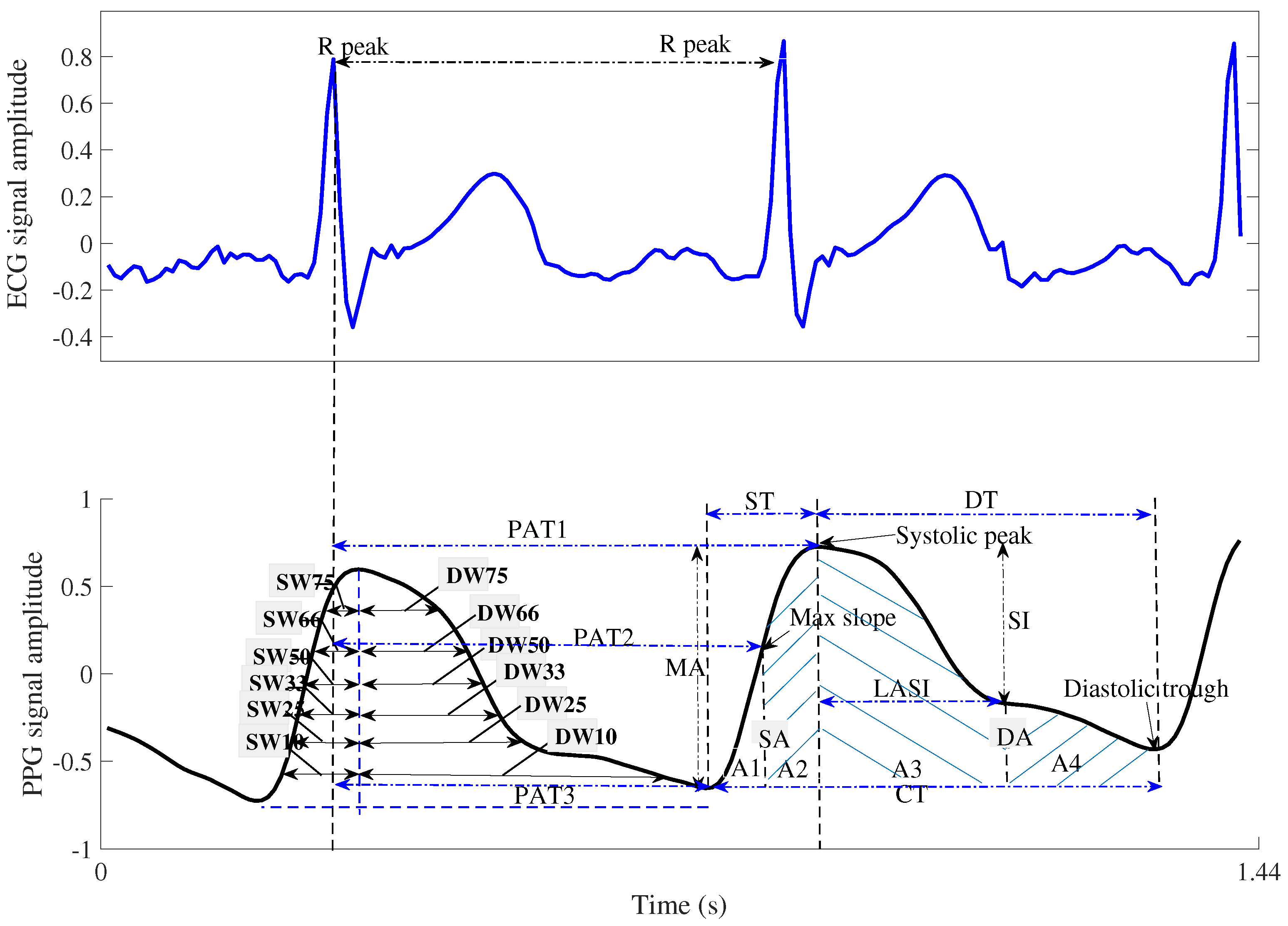
| Features | Explanation |
|---|---|
| ST: Systolic time | Rise time from the PPG trough to the PPG peak, where the PPG peak is considered the systolic point of the ABP signal [10,31]. |
| DT: Diastolic time | The time taken to fall from the current PPG waveform peak point to the next PPG waveform trough [10,31] |
| PIR: Pulse intensity ratio | Ratio of PPG peaks and troughs in the PPG [10,31] |
| HR: Heart rate | The reciprocal value of the time between consecutive ECG R-peaks [10,31] |
| PAT1: Pulse arrival time1 | The time interval between the R-peak of the ECG waveform and the peak of the PPG waveform [31] |
| PAT2: Pulse arrival time2 | The time interval between the R-peak of the ECG waveform and the maximum slope point (the first derivative peak value) of the PPG waveform [31] |
| PAT3: Pulse arrival time3 | Width between R-peak of ECG and PPG trough [31] |
| LASI: Large artery stiffness index | The reciprocal value of the period from the peak of the PPG waveform to the inflection point closest to the diastolic trough [31] |
| AUI: Augmentation index | The ratio of the peak intensity of the PPG waveform to the intensity of the inflection point near the diastolic peak of the PPG, |
| where this characteristic is considered a measure of the pressure wave reflection in the artery [31] | |
| A1 | Area under the PPG waveform curve from the diastolic trough to the maximum slope of the PPG waveform [31] |
| A2 | Area under the curve from the point of maximum slope of the PPG waveform to the peak of the PPG waveform [31] |
| A3 | Area under the curve from the PPG peak to the point of inflection closest to the diastolic peak |
| A4 | Area under the curve from the inflection point of the PPG waveform to the diastolic trough of the next PPG waveform [31] |
| IPAR: Inflection point area ratio | ratio of S4/(S1 + S2 + S3) [31] |
| dPPG height (H) | PPG’s 1st derivative characteristics [10,31] |
| dPPG width (W) | PPG’s 1st derivative characteristics [10,31] |
| PH: ddPPG peak height | PPG’s 2nd derivative characteristics [10,31] |
| TH: ddPPG trough height (TH) | PPG’s 2nd derivative characteristics [10,31] |
| W: ddPPG width | PPG’s 2nd derivative characteristics [10,31] |
| H: ddPPG height | PPG’s 2nd derivative characteristics [10,31] |
| SA | Systolic area as Figure 3 [10] |
| DA | Diastolic area as Figure 3 [10] |
| areaPPG | Area under the envelope from the PPG |
| IBI | The first PPG’s systolic peak to the second PPG’s systolic peak |
| MXAP | Maximum amplitude of PPG waveform [32] |
| MIAP | Minimum amplitude of PPG waveform [32] |
| MEU | The blood’s viscosity [32] |
| FHR | The HR’s frequency [32] |
| CT: | Cycle time of one PPG waveform |
| MPSD: | Estimated max power spectral density (PSD) |
| MCORR: | Maximum correlation between PPG waveform and ABP waveform |
| Skew | PPG waveform skewness |
| Kurt | PPG waveform kurtosis |
| Entr | PPG waveform entropy |
| and : | the widths 10% of systolic and diastolic areas as Figure 3 [10] |
| and : | the widths 25% of systolic and diastolic areas as Figure 3 |
| and : | the widths 33% of systolic and diastolic areas as Figure 3 |
| and : | the widths 50% of systolic and diastolic areas as Figure 3 |
| and : | the widths 66% of systolic and diastolic areas as Figure 3 |
| and : | the widths 75% of systolic and diastolic areas as Figure 3 |
| Parameters Combined | SVM [38] DPFE | NN [10] DPFE | DNN [45] DPFE | RTree [39] DPFE | RF [42] DPFE | GPR [15] DPFE | GPR [15] DPFE&WFD |
|---|---|---|---|---|---|---|---|
| Number of sample | 47,270 | 47,270 | 47,270 | 47,270 | 47,270 | 47,270 | 47,270 |
| Number of validation sample | 5908 | 5908 | 5908 | 5908 | 5908 | 5908 | 5908 |
| Number of testing sample | 5909 | 5909 | 5909 | 5909 | 5909 | 5909 | 5909 |
| Number of feature | 47 | 47 | 47 | 47 | 47 | 47 | 44 |
| Output dimension | 1 | 1 | 1 | 1 | 1 | 1 | 1 |
| Learner | Tree | Tree | |||||
| Learning Cycle | 30 | ||||||
| MaxNumSplits | 47,269 | ||||||
| MinLeafSize | 2 | 8 | |||||
| KFold | 10 | 10 | 10 | ||||
| LayerSize | 3 | ||||||
| Activations | ReLU | ||||||
| Lambda | 0.00001 | ||||||
| Standardize | 1 | 1 | 1 | 1 | |||
| Optimizer | Adam | ||||||
| BoxConstraint | 613 | ||||||
| Epsilon | 0.2 | 1.0 × | |||||
| KernelScale | 2.72 | ||||||
| KernelFunction | Gauss. | Exponential | Exponential | ||||
| BasicFunction | None | None | |||||
| NumHiddenUnits | 500 | ||||||
| Layer | FeatureInputLayer | ||||||
| LstmLayer | |||||||
| FullyConnectedLayer | |||||||
| MaxEpochs | 500 | ||||||
| InitialLearnRate | 0.005 | ||||||
| DropFactor | 0.1 | ||||||
| Loss | mse | ||||||
| SequenceLength | shortest |
| Methods Combined | SVM [38] DPFE | NN [10] DPFE | DNN [45] DPFE | RTree [39] DPFE | RF [42] DPFE | GPR [15] DPFE | GPR [15] DPFE&WFD |
|---|---|---|---|---|---|---|---|
| Training time (s) | 5217.4 | 41.8 | 10,875.4 | 48.1 | 128.1 | 14,533.6 | 15,576.2 |
| Validation time (s) | 8.5 | 2.5 | 3.3 | 1.8 | 2.6 | 4.30 | 4.41 |
| (mmHg) | Mean (mmHg) | SD (mmHg) | Mini (mmHg) | Max (mmHg) | ≥160 | ≥140 | ≤100 | ≥100 | ≥85 | ≤60 |
|---|---|---|---|---|---|---|---|---|---|---|
| SBP | 133.1 | 24.8 | 71.2 | 199.7 | 15.6% | 40.4% | 9.2% | |||
| DBP | 69.3 | 14.6 | 49.9 | 149.5 | 3.8% | 14.3% | 32.9% | |||
| AAMI/ESH/ISO | 5% | 20% | 5% | 5% | 20% | 5% |
| Method Combined (mmHg) | SVM [38] DPFE | NN [10] DPFE | DNN [45] DPFE | RTree [39] DPFE | RF [42] DPFE | GPR [15] DPFE | GPR [15] DPFE&WFD | |||||||
|---|---|---|---|---|---|---|---|---|---|---|---|---|---|---|
| SBP | DBP | SBP | DBP | SBP | DBP | SBP | DBP | SBP | DBP | SBP | DBP | SBP | DBP | |
| ME | −0.16 | −0.08 | −1.05 | −1.22 | 0.83 | −0.07 | −0.11 | −0.02 | −0.31 | −0.10 | −0.10 | −0.03 | −0.13 | −0.04 |
| SD | 4.30 | 2.18 | 12.17 | 6.89 | 7.92 | 3.68 | 5.76 | 2.96 | 5.08 | 2.55 | 3.18 | 1.59 | 2.94 | 1.50 |
| Method | Combined | SBP | DBP | SBP/DBP | ||||
|---|---|---|---|---|---|---|---|---|
| Mean Absolute Difference (%) | Mean Absolute Difference (%) | BHS | ||||||
| ≤5 mmHg | ≤10 mmHg | ≤15 mmHg | ≤5 mmHg | ≤10 mmHg | ≤15 mmHg | Grade | ||
| SVM | DPFE | 92.33 | 97.16 | 98.27 | 97.02 | 98.80 | 99.53 | A/A |
| NN | DPFE | 40.32 | 69.64 | 82.94 | 71.01 | 90.82 | 96.63 | C/A |
| DNN | DPFE | 51.90 | 81.71 | 93.64 | 86.74 | 97.98 | 99.46 | B/A |
| RTree | DPFE | 85.41 | 94.06 | 96.68 | 94.40 | 98.19 | 99.41 | A/A |
| RF | DPFE | 82.02 | 94.34 | 97.85 | 95.29 | 98.83 | 99.54 | A/A |
| GPR | DPFE | 93.62 | 97.95 | 99.10 | 98.15 | 99.59 | 99.86 | A/A |
| GPR | DPFE&WFD | 94.18 | 98.26 | 99.37 | 98.27 | 99.66 | 99.88 | A/A |
| Grade A | 60 | 85 | 95 | 60 | 85 | 95 | [49] | |
| Grade B | 50 | 75 | 90 | 50 | 75 | 90 | ||
| Grade C | 40 | 65 | 85 | 40 | 65 | 85 | ||
| BP (mmHg) n (=) | SBP (SD) 95%CI | DBP (SD) 95%CI | SBP L (SD) | SBP U (SD) | DBP L (SD) | DBP U (SD) |
|---|---|---|---|---|---|---|
| 5.3 (7.1) | 3.3 (3.9) | 140.4 (18.5) | 145.7 (18.0) | 74.1 (10.4) | 77.4 (10.5) | |
| 10.4 (7.2) | 4.9 (4.1) | 137.9 (18.5) | 148.3 (17.7) | 73.4 (10.7) | 78.3 (10.9) | |
| 10.8 (7.3) | 5.9 (4.0) | 135.5 (20.1) | 146.3 (20.3) | 72.2 (12.6) | 78.1 (12.5) | |
| 4.7 (6.9) | 3.0 (3.9) | 140.7 (18.7) | 145.4 (18.0) | 74.3 (10.5) | 77.3 (10.5) | |
| 8.9 (7.2) | 6.4 (4.5) | 138.6 (19.5) | 147.5 (18.4) | 72.6 (10.8) | 79.0 (10.9) | |
| 0.6 (0.9) | 0.3 (0.8) | 142.7 (18.2) | 143.3 (18.1) | 75.7 (10.4) | 76.0 (10.5) | |
| (ex1.subject) | 3.9 (1.5) | 1.6 (0.4) | 138.5 (1.1) | 142.4 (0.5) | 65.6 (0.3) | 67.2 (0.6) |
| (ex1.subject) | 5.4 (1.1) | 4.2 (0.4) | 137.8 (0.8) | 143.2 (0.3) | 64.3 (0.3) | 68.5 (0.6) |
| (ex2.subject) | 4.8 (1.9) | 2.7 (1.0) | 88.6 (1.9) | 93.4 (2.9) | 50.9 (0.9) | 53.6 (1.3) |
| (ex2.subject) | 8.6 (2.9) | 6.4 (1.3) | 86.8 (1.9) | 95.4 (3.4) | 50.2 (1.6) | 56.6 (2.1) |
Disclaimer/Publisher’s Note: The statements, opinions and data contained in all publications are solely those of the individual author(s) and contributor(s) and not of MDPI and/or the editor(s). MDPI and/or the editor(s) disclaim responsibility for any injury to people or property resulting from any ideas, methods, instructions or products referred to in the content. |
© 2025 by the authors. Licensee MDPI, Basel, Switzerland. This article is an open access article distributed under the terms and conditions of the Creative Commons Attribution (CC BY) license (https://creativecommons.org/licenses/by/4.0/).
Share and Cite
Lee, S.; Al-antari, M.A.; Joshi, G.P. Improved Confidence-Interval Estimations Using Uncertainty Measure and Weighted Feature Decisions for Cuff-Less Blood-Pressure Measurements. Bioengineering 2025, 12, 131. https://doi.org/10.3390/bioengineering12020131
Lee S, Al-antari MA, Joshi GP. Improved Confidence-Interval Estimations Using Uncertainty Measure and Weighted Feature Decisions for Cuff-Less Blood-Pressure Measurements. Bioengineering. 2025; 12(2):131. https://doi.org/10.3390/bioengineering12020131
Chicago/Turabian StyleLee, Soojeong, Mugahed A. Al-antari, and Gyanendra Prasad Joshi. 2025. "Improved Confidence-Interval Estimations Using Uncertainty Measure and Weighted Feature Decisions for Cuff-Less Blood-Pressure Measurements" Bioengineering 12, no. 2: 131. https://doi.org/10.3390/bioengineering12020131
APA StyleLee, S., Al-antari, M. A., & Joshi, G. P. (2025). Improved Confidence-Interval Estimations Using Uncertainty Measure and Weighted Feature Decisions for Cuff-Less Blood-Pressure Measurements. Bioengineering, 12(2), 131. https://doi.org/10.3390/bioengineering12020131