

Multivariate Analyses with Two-Step Dimension Reduction for an Association Study Between 11C-Pittsburgh Compound B and Magnetic Resonance Imaging in Alzheimer’s Disease

Abstract

1. Introduction
2. Materials and Methods
2.1. Data
2.2. Preprocessing
2.3. Notation
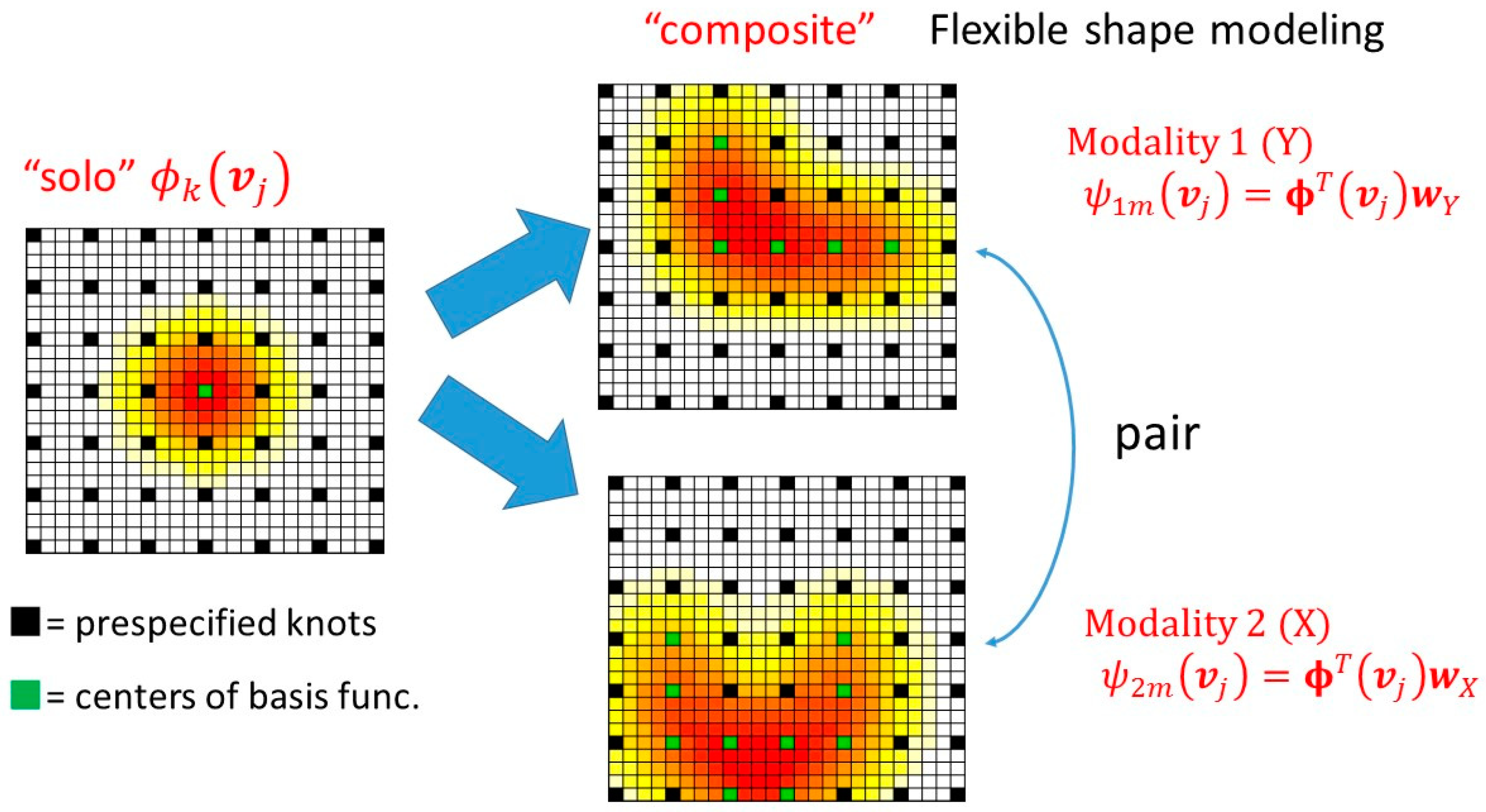
2.4. Dimension Reduction
2.5. Supervised Sparse Multivariate Analysis
- Initialize and and normalize the super scores as follows:where means “replaced with”.
- Repeat until convergence.
- 2.1
- For fixed , and normalize = .
- 2.2
- Putting , then normalize = .
- 2.3
- Set ,
- Set and , and
2.6. Statistical Analysis
2.7. Simulation Study Setting
3. Results
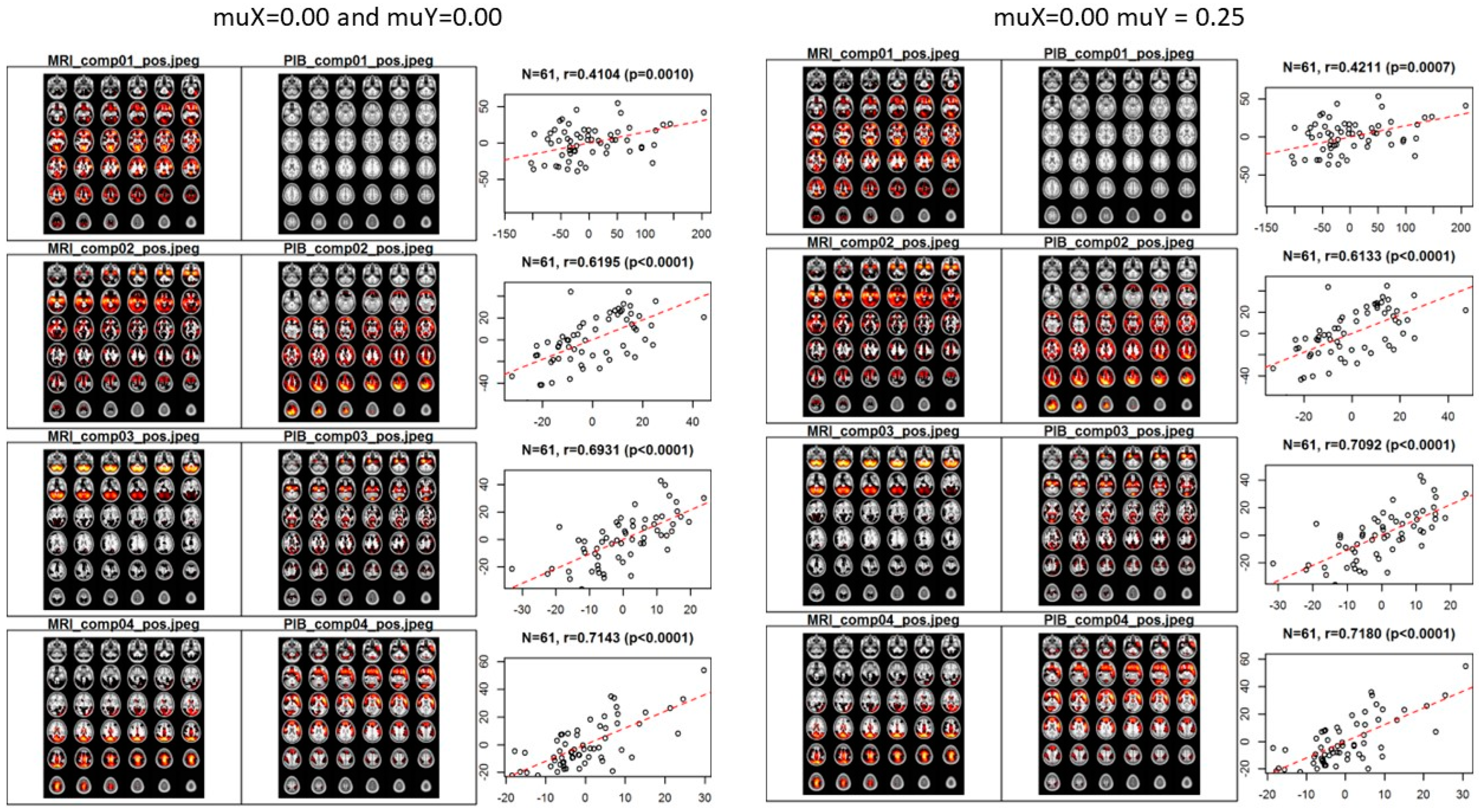
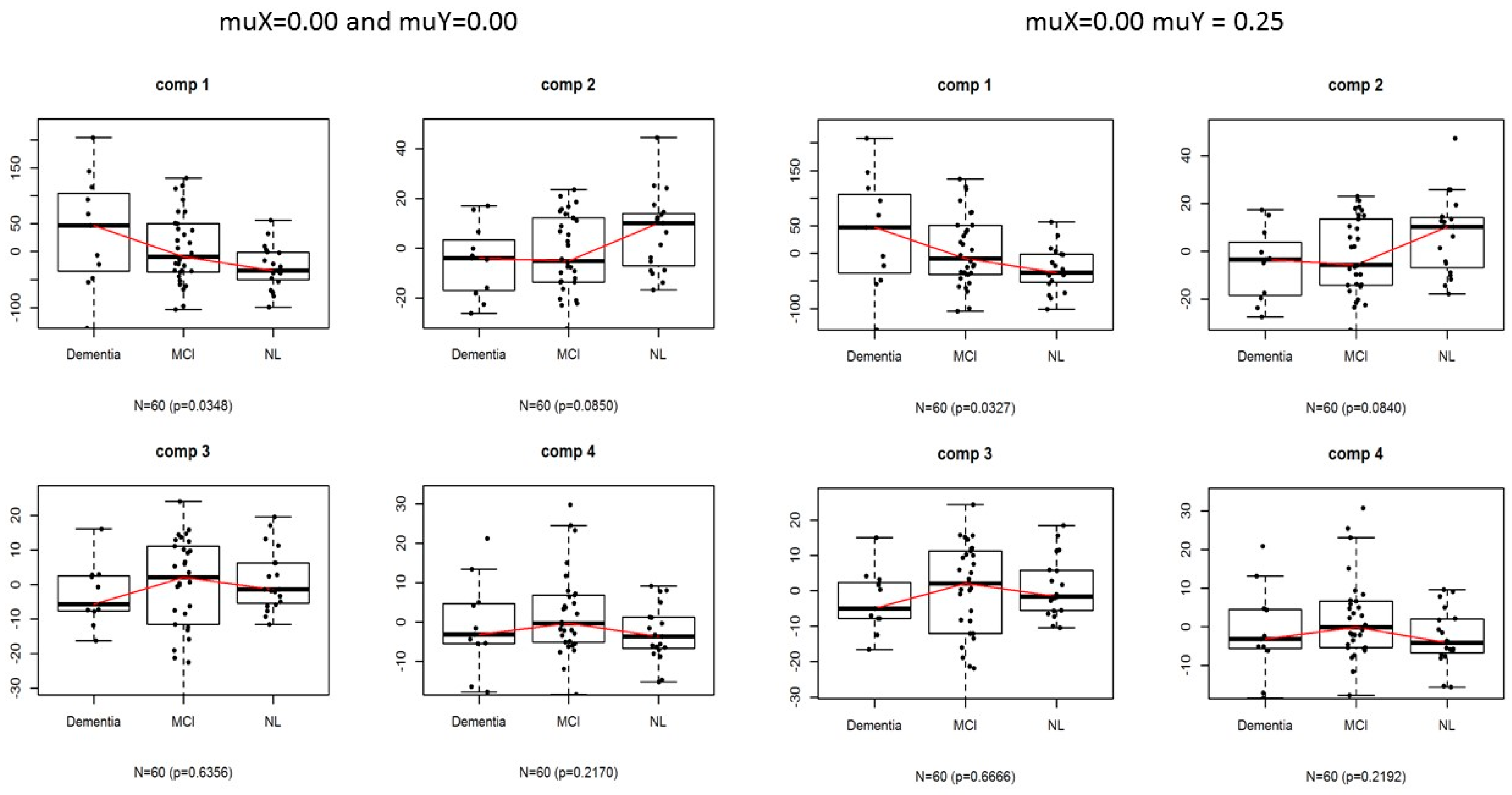
3.1. Application
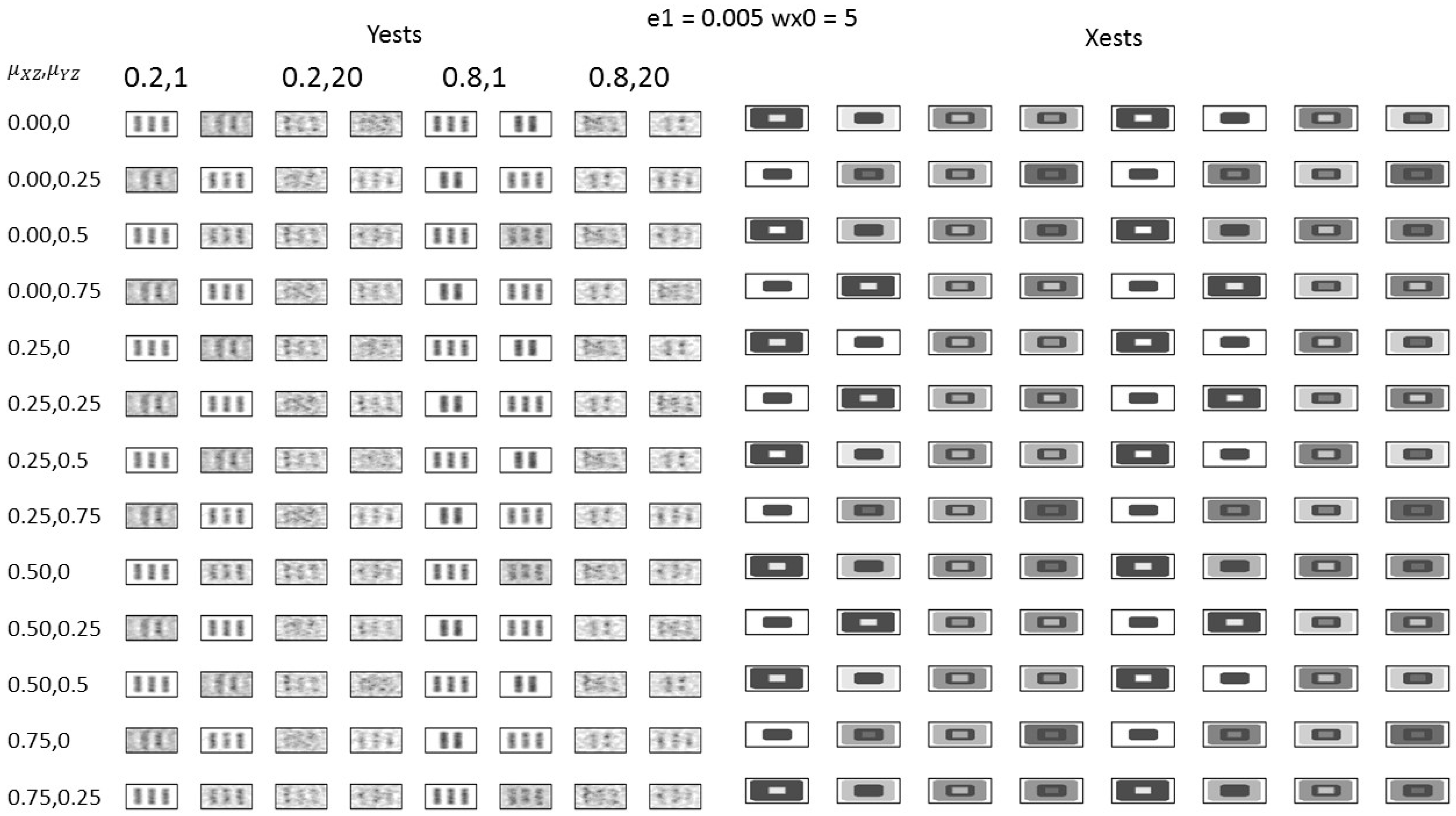
3.2. Simulation Study
4. Discussion
5. Conclusions
Author Contributions
Funding
Institutional Review Board Statement
Informed Consent Statement
Data Availability Statement
Acknowledgments
Conflicts of Interest
Appendix A

| comp1 | comp2 | Xmean | comp1 | comp2 | Ymean | XYmean | |
|---|---|---|---|---|---|---|---|
| 0.00, 0 | 0.502 | 0.844 | 0.673 | 0.432 | 0.140 | 0.286 | 0.480 |
| 0.00, 0.25 | 0.504 | 0.829 | 0.666 | 0.439 | 0.139 | 0.289 | 0.478 |
| 0.00, 0.5 | 0.501 | 0.841 | 0.671 | 0.440 | 0.136 | 0.288 | 0.479 |
| 0.00, 0.75 | 0.504 | 0.800 | 0.652 | 0.437 | 0.132 | 0.284 | 0.468 |
| 0.25, 0 | 0.506 | 0.848 | 0.677 | 0.437 | 0.139 | 0.288 | 0.482 |
| 0.25, 0.25 | 0.503 | 0.841 | 0.672 | 0.439 | 0.136 | 0.288 | 0.480 |
| 0.25, 0.5 | 0.502 | 0.818 | 0.660 | 0.435 | 0.130 | 0.282 | 0.471 |
| 0.25, 0.75 | 0.336 | 0.634 | 0.485 | 0.297 | −0.024 | 0.137 | 0.311 |
| 0.50, 0 | 0.505 | 0.842 | 0.674 | 0.433 | 0.139 | 0.286 | 0.480 |
| 0.50, 0.25 | 0.503 | 0.829 | 0.666 | 0.436 | 0.139 | 0.287 | 0.477 |
| 0.50, 0.5 | 0.336 | 0.634 | 0.485 | 0.297 | −0.024 | 0.137 | 0.311 |
| 0.75, 0 | 0.506 | 0.840 | 0.673 | 0.439 | 0.140 | 0.289 | 0.481 |
| 0.75, 0.25 | 0.336 | 0.634 | 0.485 | 0.297 | −0.024 | 0.137 | 0.311 |
| comp1 | comp2 | Xmean | comp1 | comp2 | Ymean | XYmean | |
|---|---|---|---|---|---|---|---|
| 0.00, 0 | 0.344 | 0.383 | 0.364 | 0.021 | 0.026 | 0.024 | 0.194 |
| 0.00, 0.25 | 0.367 | 0.366 | 0.367 | 0.018 | 0.028 | 0.023 | 0.195 |
| 0.00, 0.5 | 0.343 | 0.360 | 0.352 | 0.019 | 0.030 | 0.024 | 0.188 |
| 0.00, 0.75 | 0.335 | 0.344 | 0.339 | 0.022 | 0.029 | 0.025 | 0.182 |
| 0.25, 0 | 0.354 | 0.304 | 0.329 | 0.019 | 0.030 | 0.024 | 0.177 |
| 0.25, 0.25 | 0.354 | 0.313 | 0.333 | 0.019 | 0.026 | 0.022 | 0.178 |
| 0.25, 0.5 | 0.346 | 0.330 | 0.338 | 0.018 | 0.029 | 0.024 | 0.181 |
| 0.25, 0.75 | 0.383 | 0.394 | 0.388 | 0.020 | 0.015 | 0.018 | 0.203 |
| 0.50, 0 | 0.343 | 0.295 | 0.319 | 0.017 | 0.031 | 0.024 | 0.171 |
| 0.50, 0.25 | 0.356 | 0.300 | 0.328 | 0.016 | 0.028 | 0.022 | 0.175 |
| 0.50, 0.5 | 0.383 | 0.394 | 0.388 | 0.020 | 0.015 | 0.018 | 0.203 |
| 0.75, 0 | 0.346 | 0.307 | 0.327 | 0.017 | 0.032 | 0.024 | 0.176 |
| 0.75, 0.25 | 0.383 | 0.394 | 0.388 | 0.020 | 0.015 | 0.018 | 0.203 |
References
- Nichols, E.; Steinmetz, J.D.; Vollset, S.E.; Fukutaki, K.; Chalek, J.; Abd-Allah, F.; Abdoli, A.; Abualhasan, A.; Abu-Gharbieh, E.; Akram, T.T.; et al. Estimation of the global prevalence of dementia in 2019 and forecasted prevalence in 2050: An analysis for the Global Burden of Disease Study 2019. Lancet Public Health 2022, 7, e105–e125. [Google Scholar] [CrossRef] [PubMed]
- Adlard, P.A.; Tran, B.A.; Finkelstein, D.I.; Desmond, P.M.; Johnston, L.A.; Bush, A.I.; Egan, G.F. A review of β-amyloid neuroimaging in Alzheimer’s disease. Front. Neurosci. 2014, 8, 327. [Google Scholar] [CrossRef] [PubMed]
- Chapleau, M.; Iaccarino, L.; Soleimani-Meigooni, D.; Rabinovici, G.D. The role of amyloid PET in imaging neurodegenerative disorders: A review. J. Nucl. Med. 2022, 63 (Suppl. 1), 13S–19S. [Google Scholar] [CrossRef] [PubMed]
- Edison, P.; Rowe, C.C.; Rinne, J.O.; Ng, S.; Ahmed, I.; Kemppainen, N.; Villemagne, V.L.; O’Keefe, G.; Någren, K.; Chaudhury, K.R.; et al. Amyloid load in Parkinson’s disease dementia and Lewy body dementia measured with [11C] PIB positron emission tomography. J. Neurol. Neurosurg. Psychiatry 2008, 79, 1331–1338. [Google Scholar] [CrossRef] [PubMed]
- Donaghy, P.; Thomas, A.J.; O’Brien, J.T. Amyloid PET imaging in Lewy body disorders. Am. J. Geriatr. Psychiatry 2015, 23, 23–37. [Google Scholar] [CrossRef] [PubMed]
- Walker, L.; Simpson, H.; Thomas, A.J.; Attems, J. Prevalence, distribution, and severity of cerebral amyloid angiopathy differ between Lewy body diseases and Alzheimer’s disease. Acta Neuropathol. Commun. 2024, 12, 28. [Google Scholar] [CrossRef] [PubMed]
- Xin, Y.; Sheng, J.; Miao, M.; Wang, L.; Yang, Z.; Huang, H. A review of imaging genetics in Alzheimer’s disease. J. Clin. Neurosci. 2022, 100, 155–163. [Google Scholar] [CrossRef] [PubMed]
- Liu, J.; Calhoun, V.D. A review of multivariate analyses in imaging genetics. Front. Neuroinform. 2014, 8, 29. [Google Scholar] [CrossRef] [PubMed]
- Lin, D.; Cao, H.; Calhoun, V.D.; Wang, Y.P. Sparse models for correlative and integrative analysis of imaging and genetic data. J. Neurosci. Methods 2014, 237, 69–78. [Google Scholar] [CrossRef] [PubMed]
- Kawaguchi, A.; Yamashita, F. Supervised multiblock sparse multivariable analysis with application to multimodal brain imaging genetics. Biostatistics 2017, 18, 651–665. [Google Scholar] [CrossRef]
- Yoshida, H.; Kawaguchi, A.; Tsuruya, K. Radial basis function-sparse partial least squares for application to brain imaging data. Comput. Math. Methods Med. 2013, 2013, 591032. [Google Scholar] [CrossRef] [PubMed]
- Ashburner, J.; Friston, K.J. Voxel-based morphometry--The methods. Neuroimage 2000, 11, 805–821. [Google Scholar] [CrossRef] [PubMed]
- Araki, Y.; Kawaguchi, A.; Yamashita, F. Regularized logistic discrimination with basis expansions for the early detection of Alzheimer’s disease based on three-dimensional MRI data. Adv. Data Anal. Classif. 2013, 7, 109–119. [Google Scholar] [CrossRef]
- Araki, Y.; Kawaguchi, A. Functional logistic discrimination with sparse PCA and its application to the structural MRI. Behaviormetrika 2019, 46, 147–162. [Google Scholar] [CrossRef]
- Yoshida, H.; Kawaguchi, A.; Yamashita, F.; Tsuruya, K. The utility of a network–based clustering method for dimension reduction of imaging and non-imaging biomarkers predictive of Alzheimer’s disease. Sci. Rep. 2018, 8, 2807. [Google Scholar] [CrossRef]
- Kawaguchi, A. Multivariate Analysis for Neuroimaging Data; CRC Press: Boca Raton, FL, USA, 2021. [Google Scholar]
- Yokoi, T.; Watanabe, H.; Yamaguchi, H.; Bagarinao, E.; Masuda, M.; Imai, K.; Ogura, A.; Ohdake, R.; Kawabata, K.; Hara, K.; et al. Involvement of the precuneus/posterior cingulate cortex is significant for the development of Alzheimer’s disease: A PET (THK5351, PiB) and resting fMRI study. Front. Aging Neurosci. 2018, 10, 304. [Google Scholar] [CrossRef]
- Boccia, M.; Acierno, M.; Piccardi, L. Neuroanatomy of Alzheimer’s Disease and Late-Life Depression: A Coordinate-Based Meta-Analysis of MRI Studies. J. Alzheimers Dis. 2015, 46, 963–970. [Google Scholar] [CrossRef] [PubMed]
- Talwar, P.; Kushwaha, S.; Chaturvedi, M.; Mahajan, V. Systematic Review of Different Neuroimaging Correlates in Mild Cognitive Impairment and Alzheimer’s Disease. Clin. Neuroradiol. 2021, 31, 953–967. [Google Scholar] [CrossRef] [PubMed]
- Storandt, M.; Mintun, M.A.; Head, D.; Morris, J.C. Cognitive Decline and Brain Volume Loss as Signatures of Cerebral Amyloid-β Peptide Deposition Identified With Pittsburgh Compound B. Arch. Neurol. 2009, 66, 1476–1481. [Google Scholar] [CrossRef] [PubMed]

| comp1 | comp2 | Xmean | comp1 | comp2 | Ymean | XYmean | |
|---|---|---|---|---|---|---|---|
| 0.00, 0 | 0.348 | 0.351 | 0.350 | 0.021 | 0.028 | 0.024 | 0.187 |
| 0.00, 0.25 | 0.356 | 0.358 | 0.357 | 0.020 | 0.027 | 0.023 | 0.190 |
| 0.00, 0.5 | 0.355 | 0.311 | 0.333 | 0.019 | 0.028 | 0.023 | 0.178 |
| 0.00, 0.75 | 0.364 | 0.283 | 0.324 | 0.021 | 0.023 | 0.022 | 0.173 |
| 0.25, 0 | 0.349 | 0.287 | 0.318 | 0.018 | 0.026 | 0.022 | 0.170 |
| 0.25, 0.25 | 0.349 | 0.280 | 0.314 | 0.018 | 0.023 | 0.021 | 0.168 |
| 0.25, 0.5 | 0.337 | 0.283 | 0.310 | 0.019 | 0.026 | 0.022 | 0.166 |
| 0.25, 0.75 | 0.381 | 0.389 | 0.385 | 0.020 | 0.013 | 0.017 | 0.201 |
| 0.50, 0 | 0.348 | 0.294 | 0.321 | 0.017 | 0.028 | 0.022 | 0.172 |
| 0.50, 0.25 | 0.350 | 0.292 | 0.321 | 0.017 | 0.021 | 0.019 | 0.170 |
| 0.50, 0.5 | 0.381 | 0.389 | 0.385 | 0.020 | 0.013 | 0.017 | 0.201 |
| 0.75, 0 | 0.348 | 0.280 | 0.314 | 0.018 | 0.028 | 0.023 | 0.168 |
| 0.75, 0.25 | 0.381 | 0.389 | 0.385 | 0.020 | 0.013 | 0.017 | 0.201 |
| comp1 | comp2 | Xmean | comp1 | comp2 | Ymean | XYmean | |
|---|---|---|---|---|---|---|---|
| 0.00, 0 | 0.510 | 0.870 | 0.690 | 0.466 | 0.690 | 0.578 | 0.634 |
| 0.00, 0.25 | 0.504 | 0.862 | 0.683 | 0.463 | 0.690 | 0.577 | 0.630 |
| 0.00, 0.5 | 0.504 | 0.853 | 0.678 | 0.470 | 0.693 | 0.581 | 0.630 |
| 0.00, 0.75 | 0.499 | 0.853 | 0.676 | 0.473 | 0.686 | 0.580 | 0.628 |
| 0.25, 0 | 0.506 | 0.863 | 0.684 | 0.464 | 0.705 | 0.584 | 0.634 |
| 0.25, 0.25 | 0.499 | 0.864 | 0.681 | 0.460 | 0.704 | 0.582 | 0.632 |
| 0.25, 0.5 | 0.493 | 0.874 | 0.684 | 0.472 | 0.708 | 0.590 | 0.637 |
| 0.25, 0.75 | 0.375 | 0.602 | 0.489 | 0.362 | 0.008 | 0.185 | 0.337 |
| 0.50, 0 | 0.506 | 0.863 | 0.685 | 0.465 | 0.704 | 0.584 | 0.634 |
| 0.50, 0.25 | 0.489 | 0.868 | 0.679 | 0.457 | 0.701 | 0.579 | 0.629 |
| 0.50, 0.5 | 0.375 | 0.602 | 0.489 | 0.362 | 0.008 | 0.185 | 0.337 |
| 0.75, 0 | 0.505 | 0.874 | 0.690 | 0.465 | 0.704 | 0.584 | 0.637 |
| 0.75, 0.25 | 0.375 | 0.602 | 0.489 | 0.362 | 0.008 | 0.185 | 0.337 |
Disclaimer/Publisher’s Note: The statements, opinions and data contained in all publications are solely those of the individual author(s) and contributor(s) and not of MDPI and/or the editor(s). MDPI and/or the editor(s) disclaim responsibility for any injury to people or property resulting from any ideas, methods, instructions or products referred to in the content. |
© 2025 by the authors. Licensee MDPI, Basel, Switzerland. This article is an open access article distributed under the terms and conditions of the Creative Commons Attribution (CC BY) license (https://creativecommons.org/licenses/by/4.0/).
Share and Cite
Kawaguchi, A.; Yamashita, F. Multivariate Analyses with Two-Step Dimension Reduction for an Association Study Between 11C-Pittsburgh Compound B and Magnetic Resonance Imaging in Alzheimer’s Disease. Bioengineering 2025, 12, 48. https://doi.org/10.3390/bioengineering12010048
Kawaguchi A, Yamashita F. Multivariate Analyses with Two-Step Dimension Reduction for an Association Study Between 11C-Pittsburgh Compound B and Magnetic Resonance Imaging in Alzheimer’s Disease. Bioengineering. 2025; 12(1):48. https://doi.org/10.3390/bioengineering12010048
Chicago/Turabian StyleKawaguchi, Atsushi, and Fumio Yamashita. 2025. "Multivariate Analyses with Two-Step Dimension Reduction for an Association Study Between 11C-Pittsburgh Compound B and Magnetic Resonance Imaging in Alzheimer’s Disease" Bioengineering 12, no. 1: 48. https://doi.org/10.3390/bioengineering12010048
APA StyleKawaguchi, A., & Yamashita, F. (2025). Multivariate Analyses with Two-Step Dimension Reduction for an Association Study Between 11C-Pittsburgh Compound B and Magnetic Resonance Imaging in Alzheimer’s Disease. Bioengineering, 12(1), 48. https://doi.org/10.3390/bioengineering12010048