


Simple and Powerful PCG Classification Method Based on Selection and Transfer Learning for Precision Medicine Application


Abstract
1. Introduction
Contributions
- Development of a common benchmark for Physionet PCG dataset based on CNN transfer learning and fine-tuning techniques. This includes the presentation of classification results such as accuracy, sensitivity, specificity, and precision based on raw Physionet data.
- Proposal of a simple and effective classification architecture without any prepocessing steps. Our approach is based on a simple PCG data selection technique to improve the normal and abnormal Physionet signal classification results using CNN technology.
2. Related Works
3. Dataset
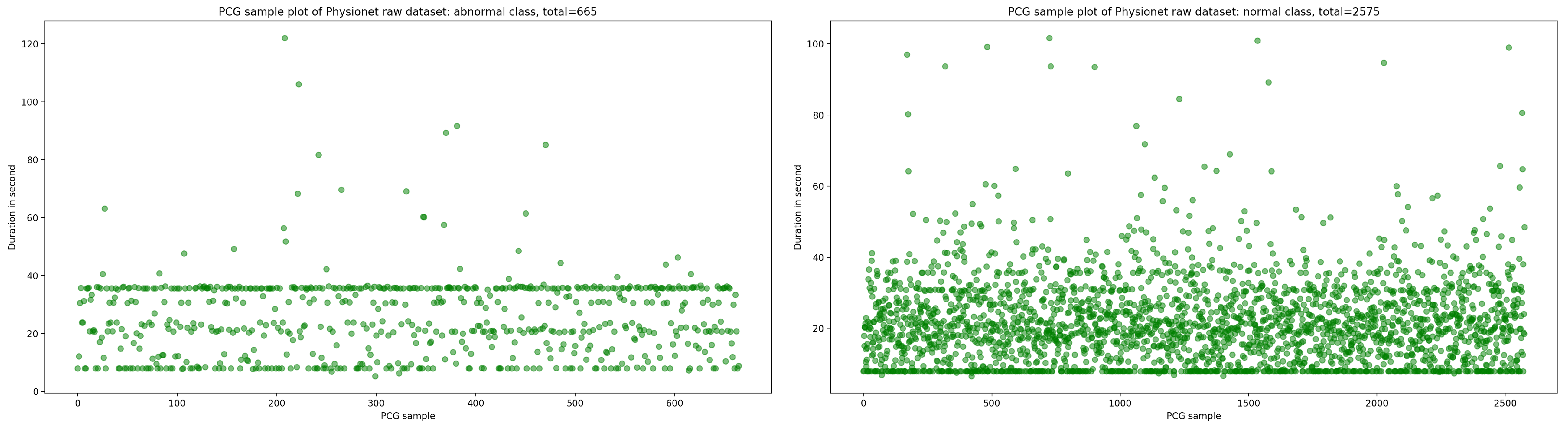
3.1. Raw Dataset
3.2. PCG Data Selection
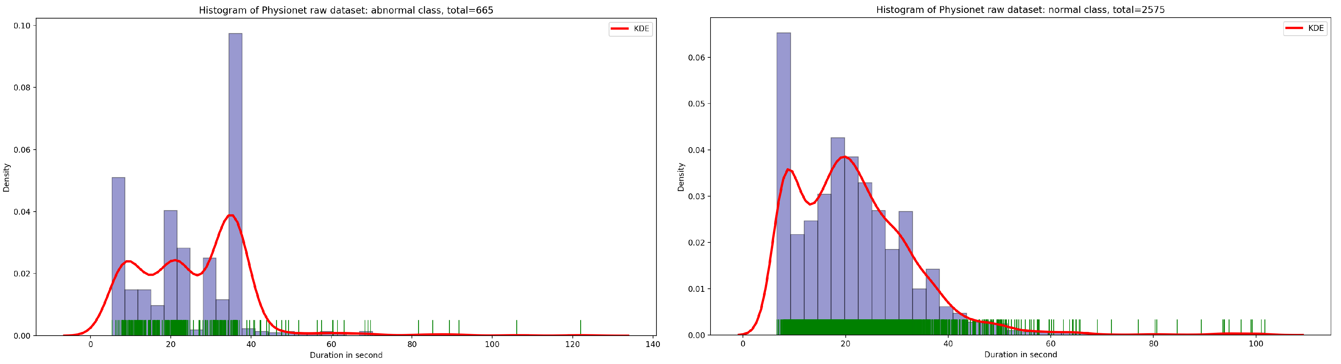
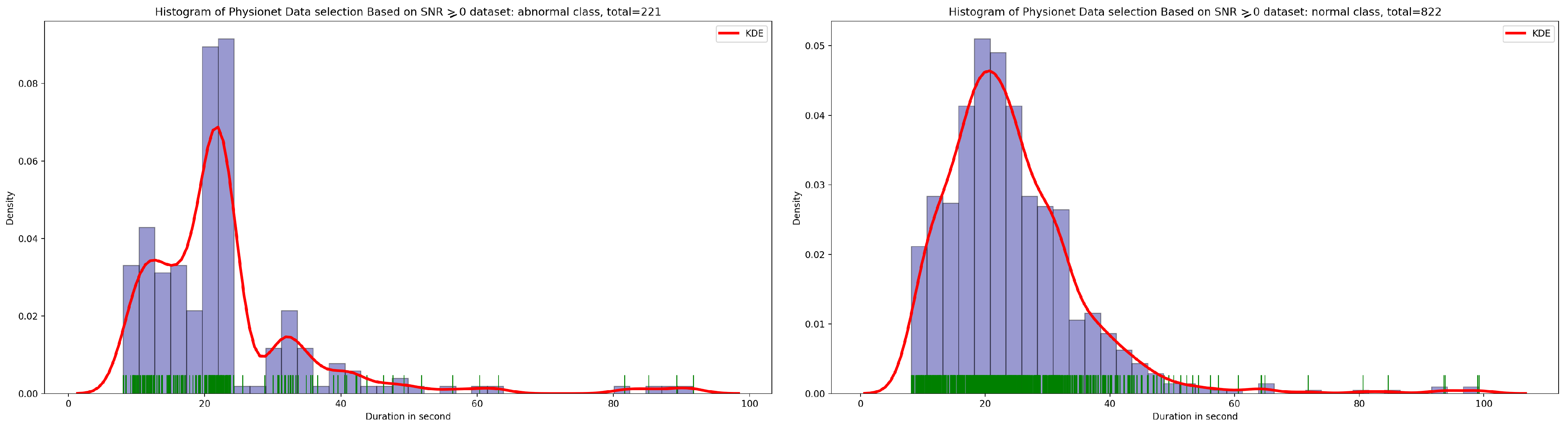
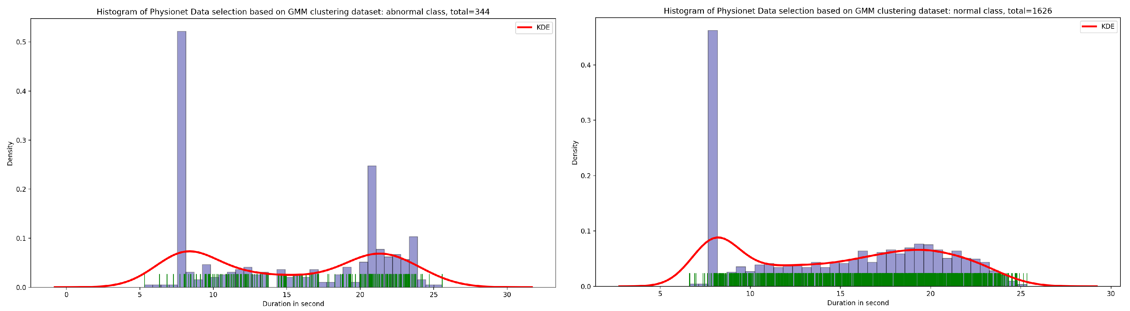
3.2.1. Data Selection Based on Kernel Density Estimation for Optimal Signal Duration Determination
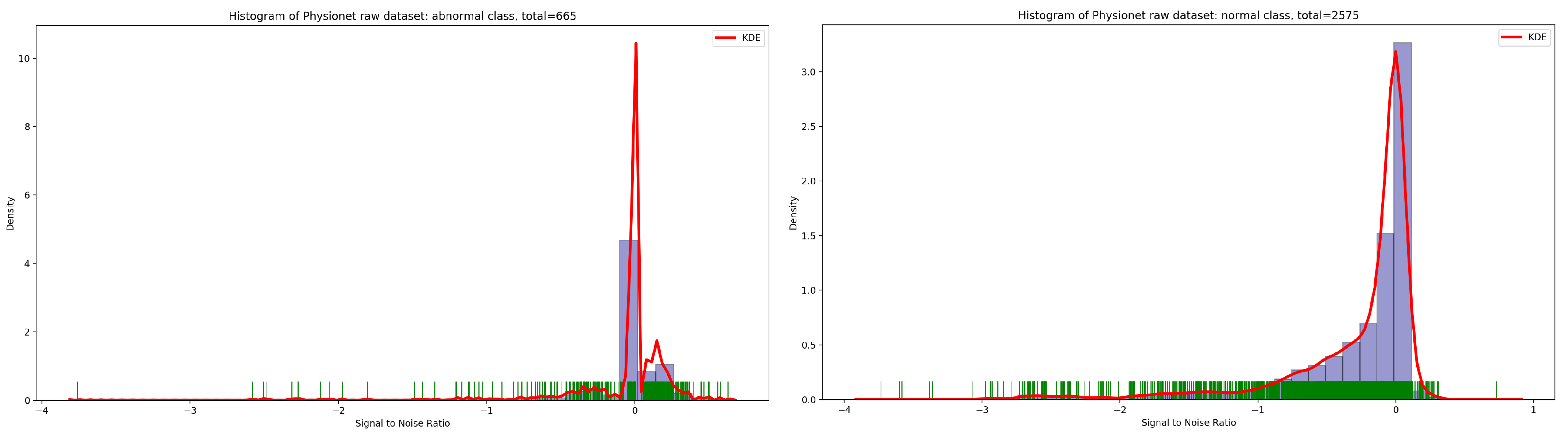
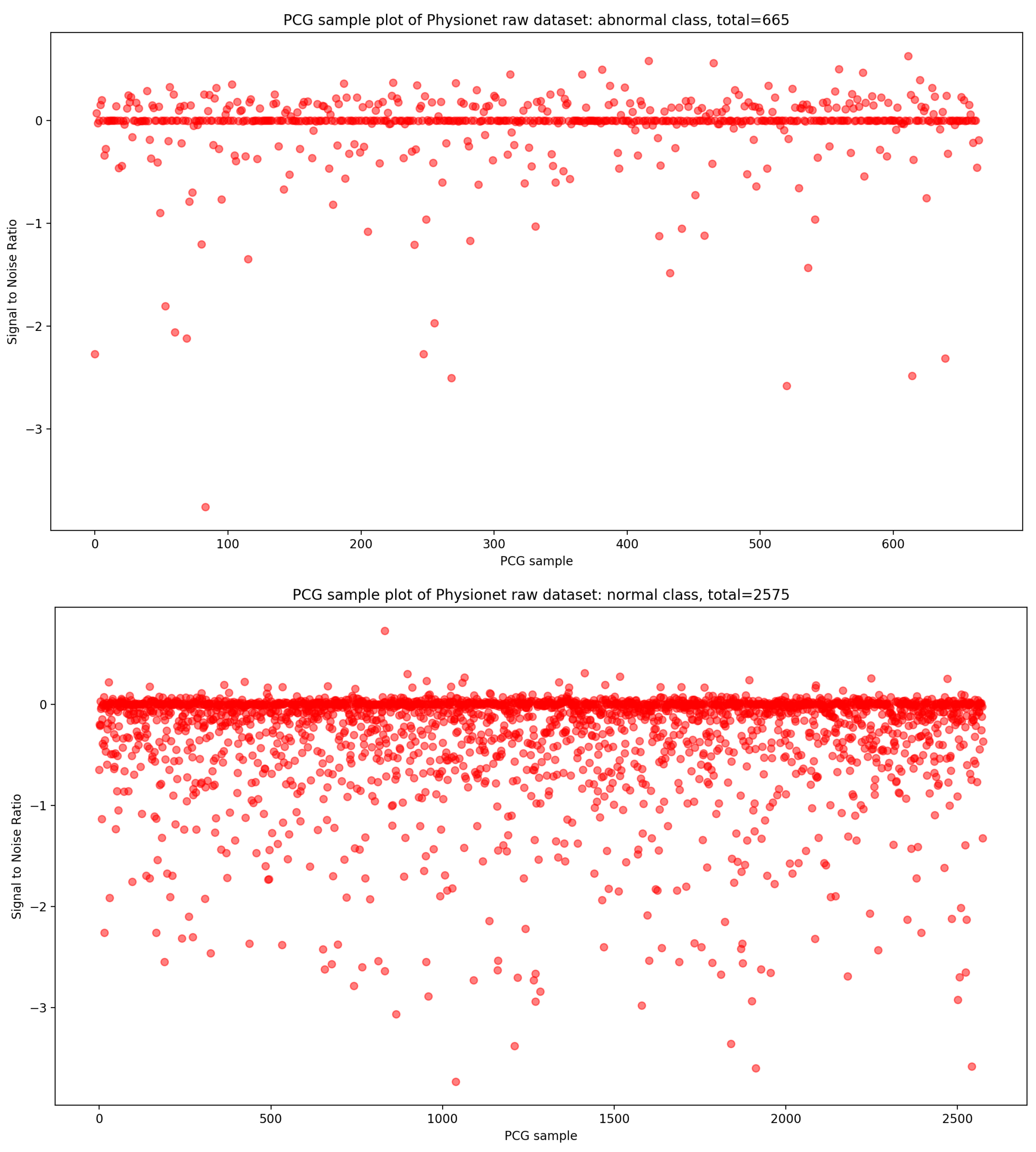
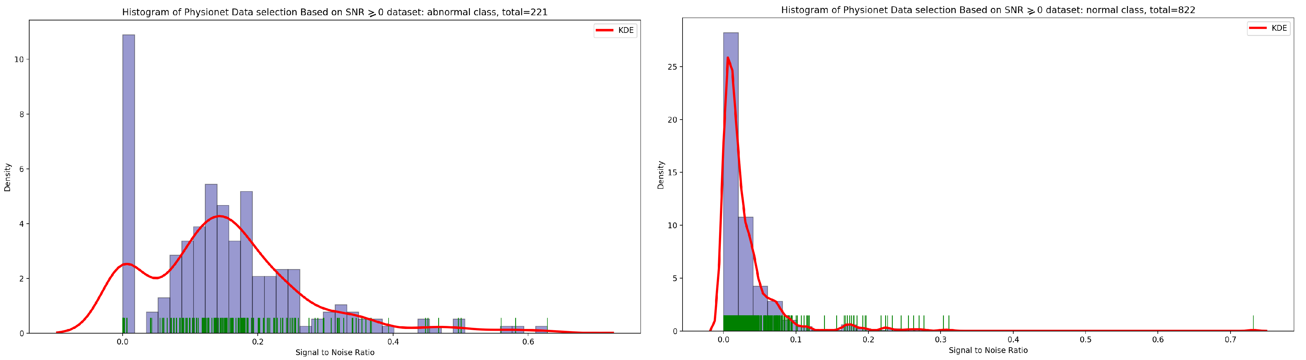
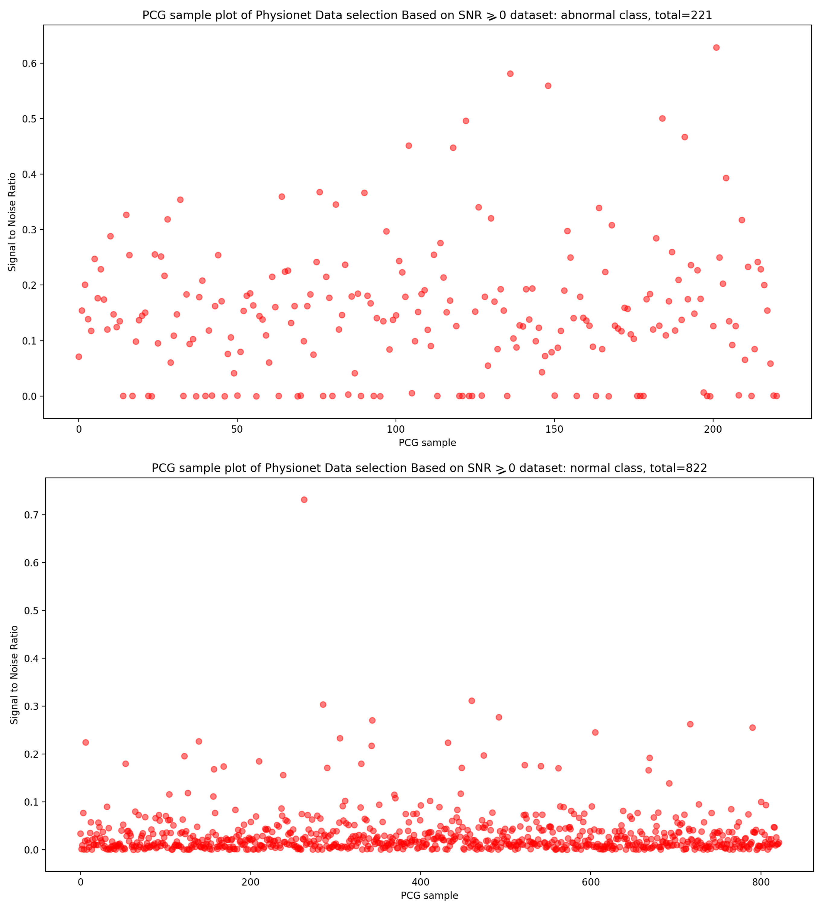
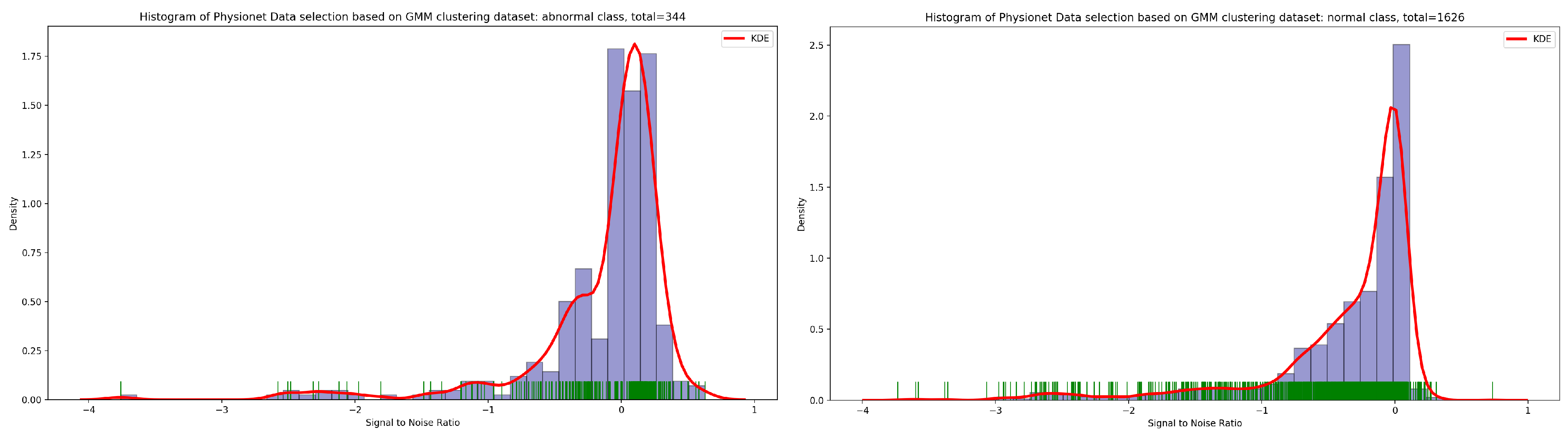
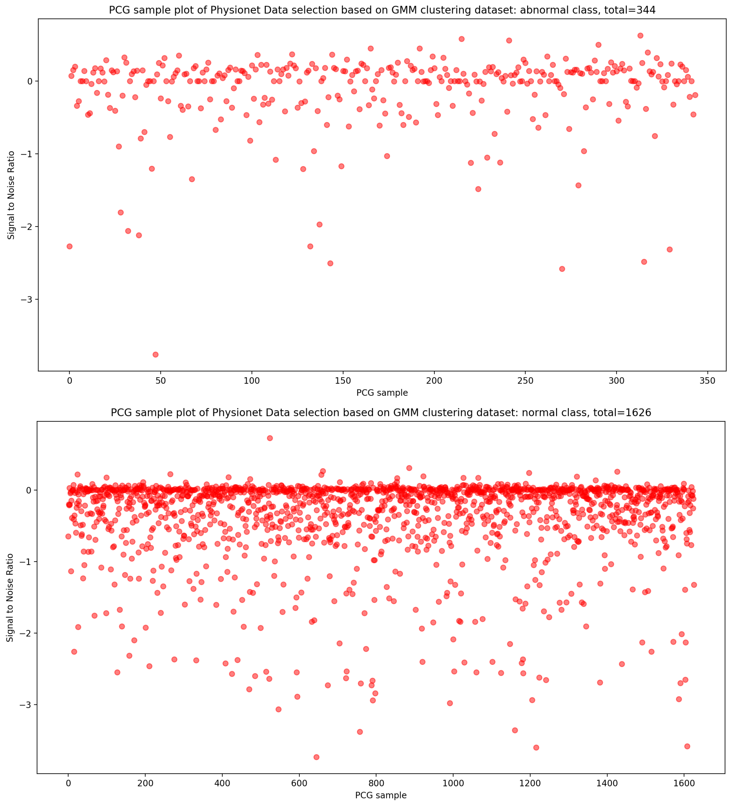
3.2.2. Data Selection Based on Optimal SNR
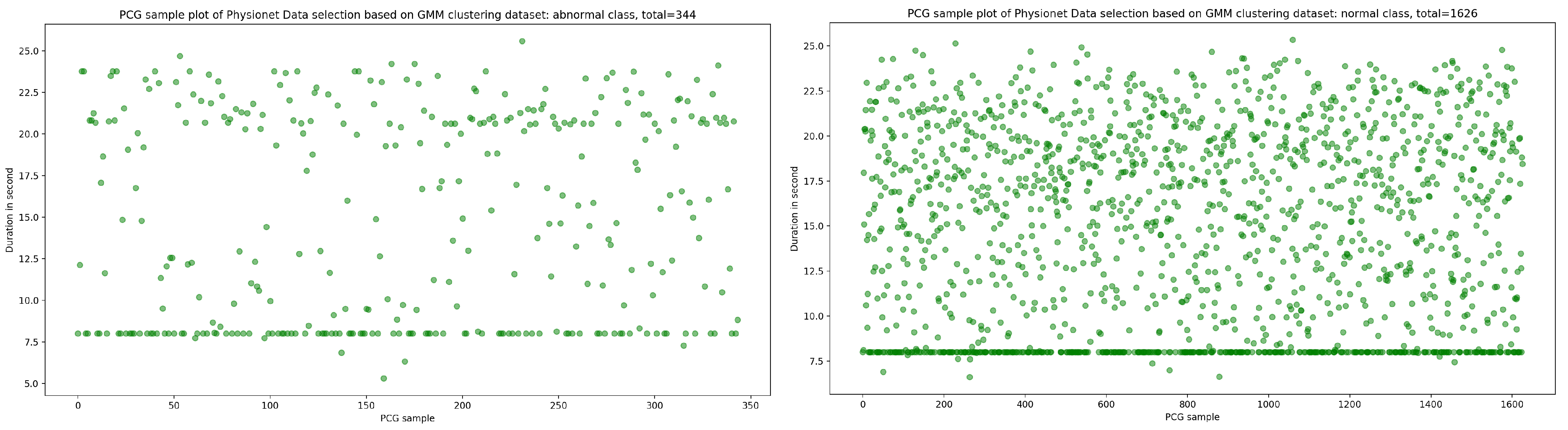
3.2.3. Data Selection Based on Clustering
- -
- Step 1: Parameter initialization
- -
- Step 2: Repeat until convergence
- Estimation step: Calculation of conditional probabilities that the sample i comes from the Gaussian k. with : the set of Gaussians.
- Maximization step: Update settings and , ,
4. The Process of Our CNN Benchmark
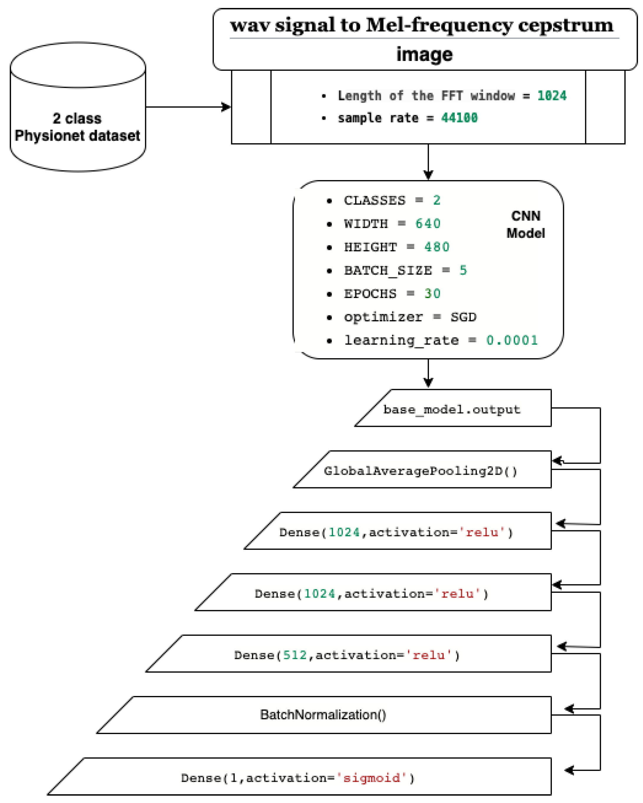
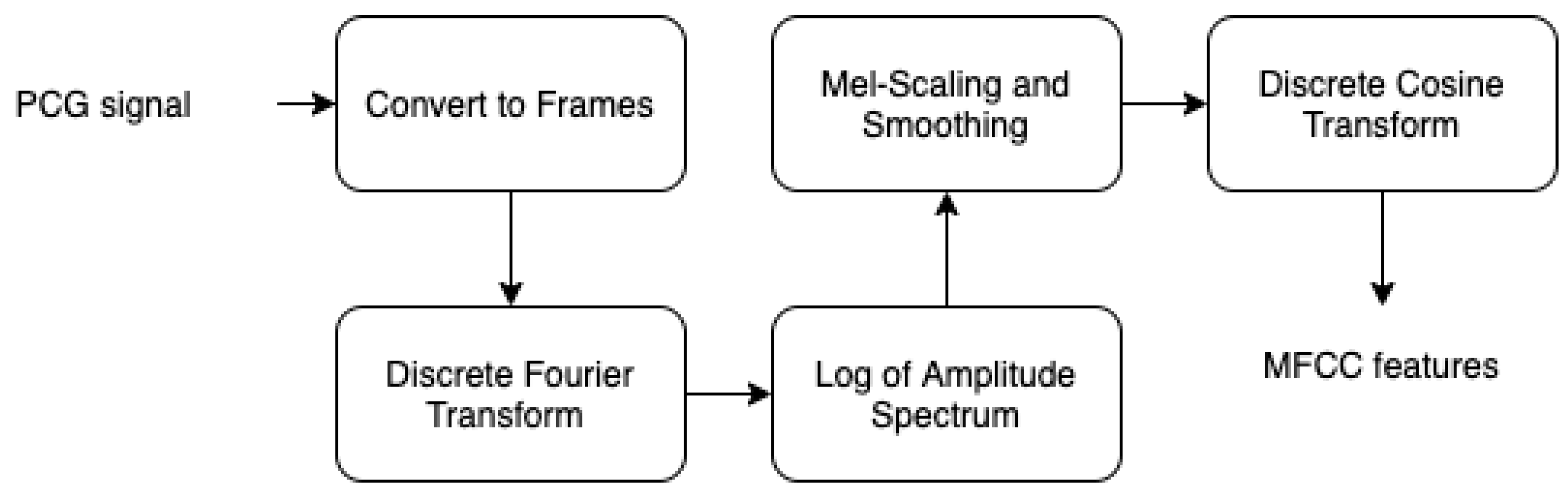
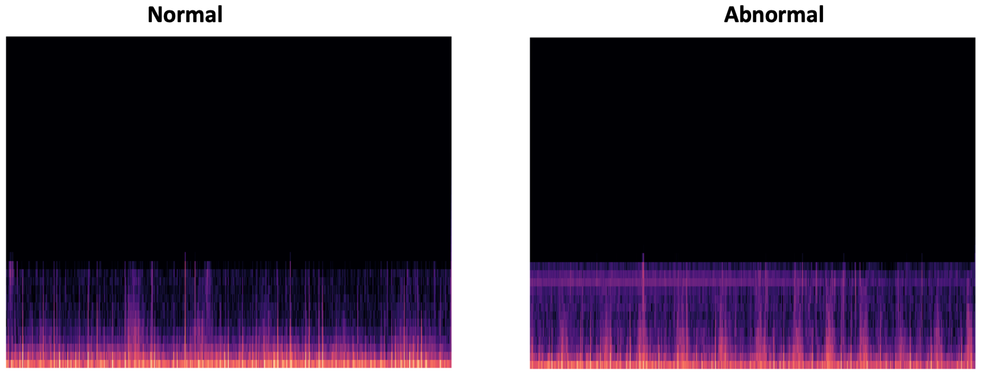
4.1. Mel Spectrogram Representation
- Specify the signal into short frames.
- Windowing in order to reduce spectral leakage.
- Work out the discrete Fourier transformation.
- Applying filter banks.
- Applying the log of the spectrogram values to obtain the log filter-bank energies.
- Applying discrete cosine transform to decorrelate the filter bank coefficients.
4.2. CNN Models
- GlobalAveragePooling2D layer for averaging and better representation of our training vector.
- Three dense layers to define our full connected network.
- BatchNormalization layer to limit covariate shift by normalizing the activations of each layer.
- Dense layer with sigmoid activation function in order to obtain classification values between 0 and 1 (probability).
- Raw PhysioNet dataset.
- PhysioNet dataset with data selection using KDE for duration extraction.
- PhysioNet dataset with data selection using optimal SNR.
- PhysioNet dataset with data selection using GMM biclustering.
5. Experiments and Results
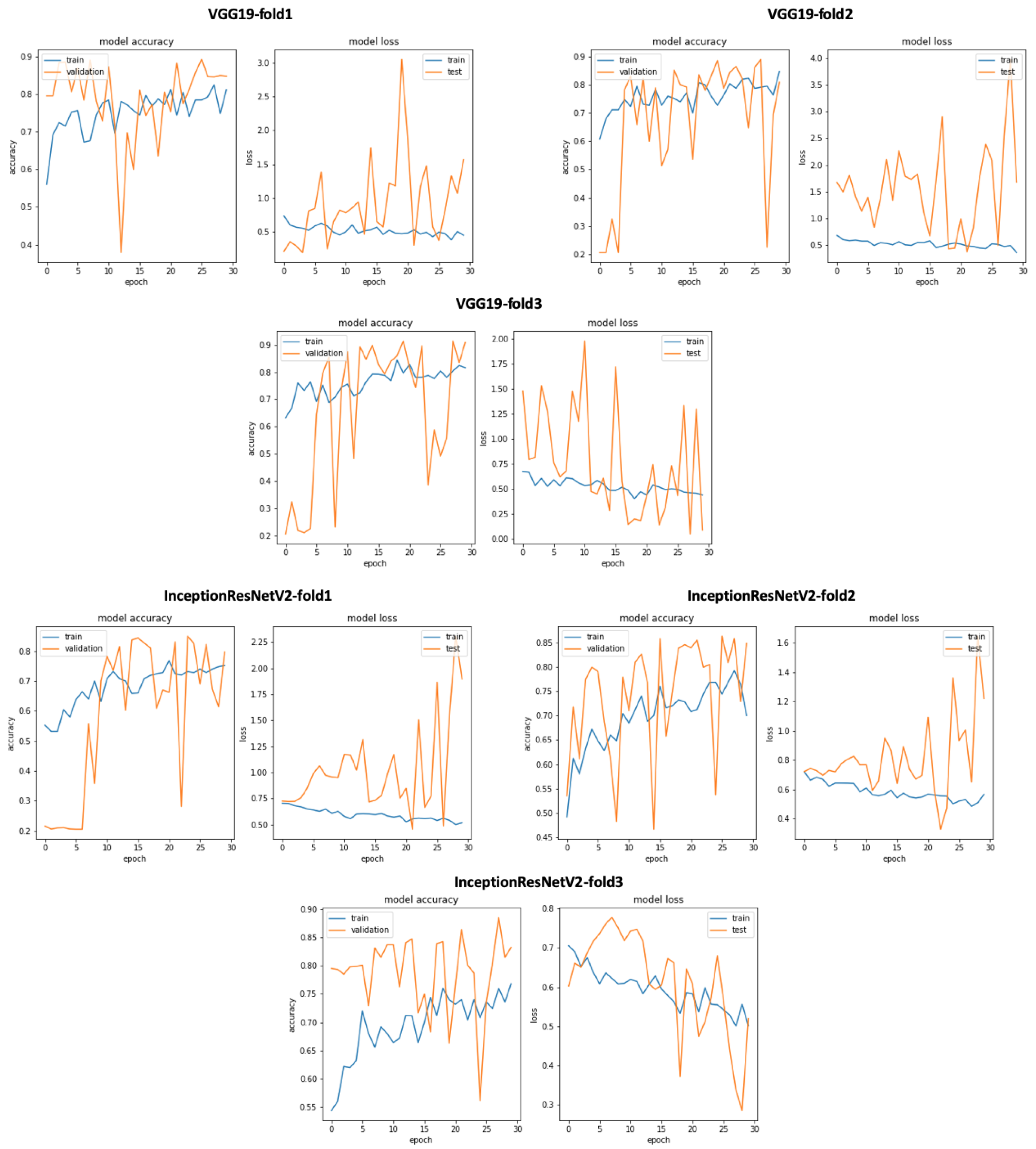
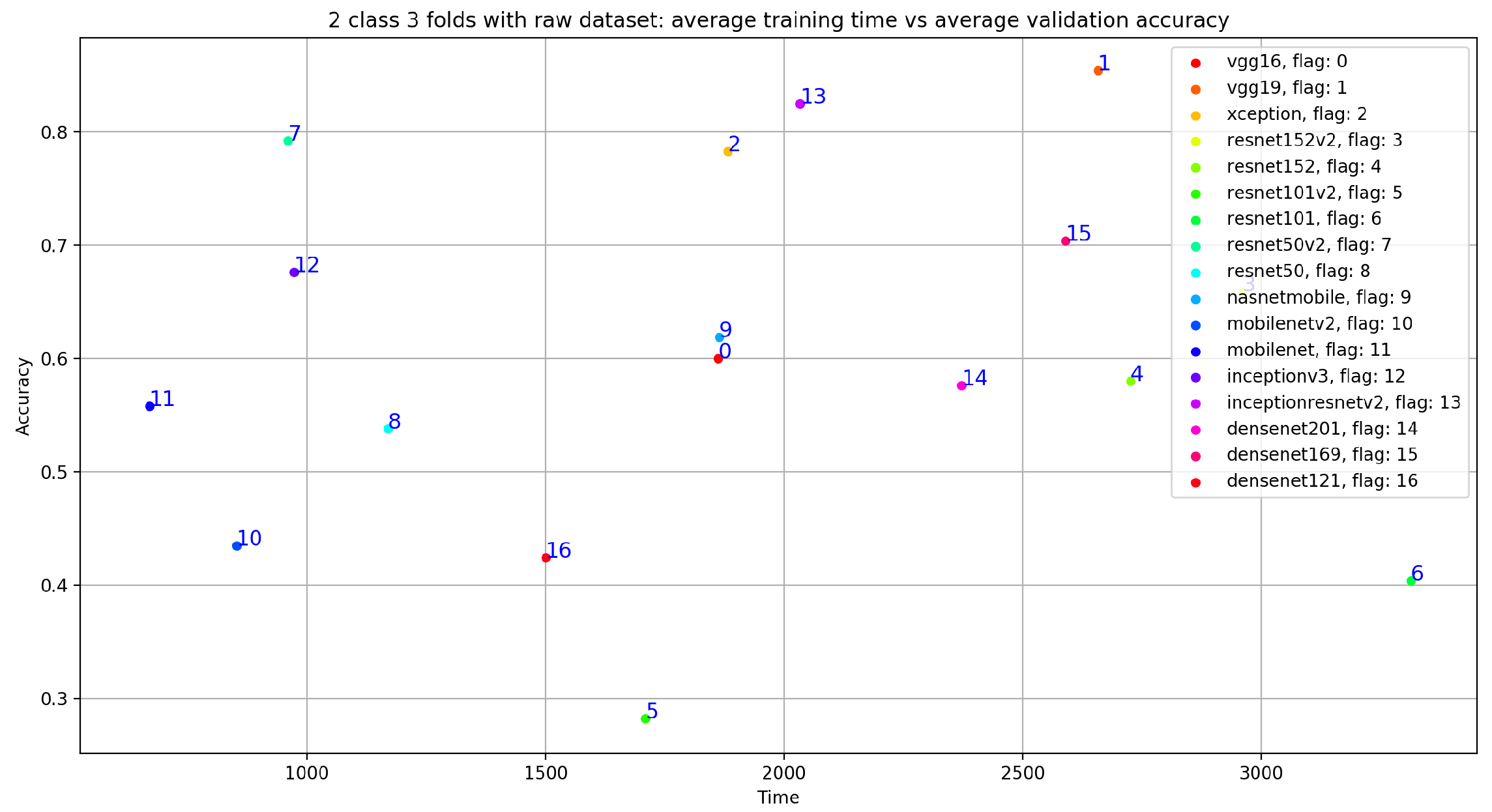
5.1. Classification Using Raw Dataset
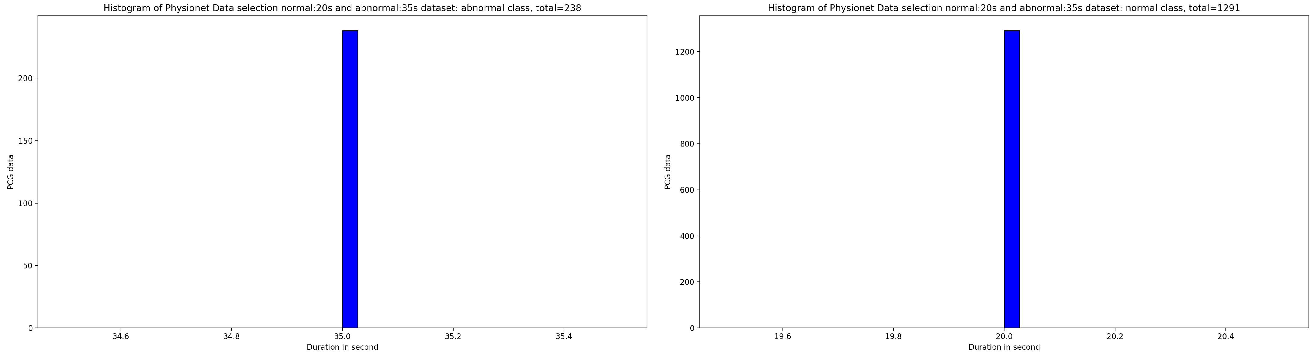
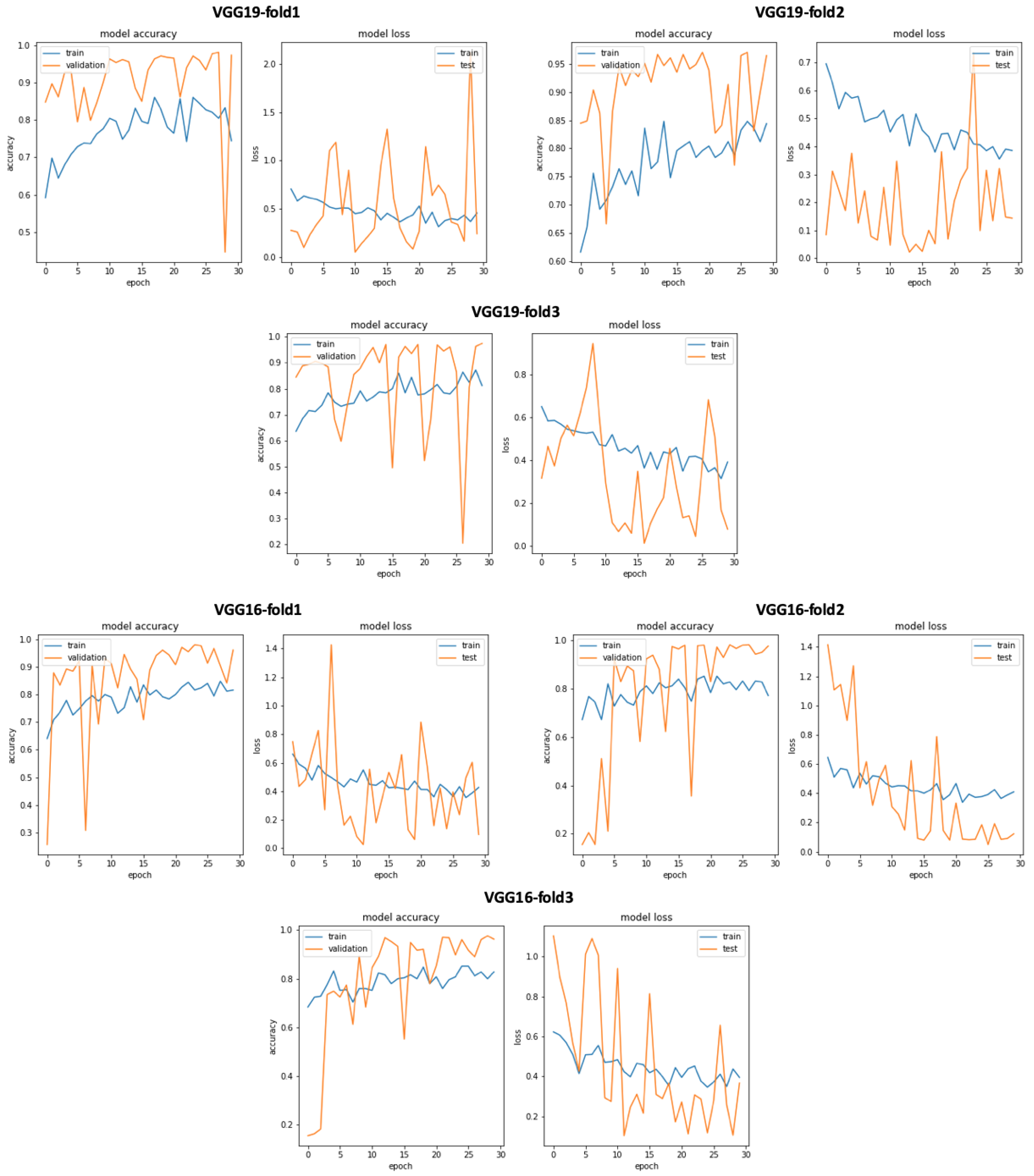
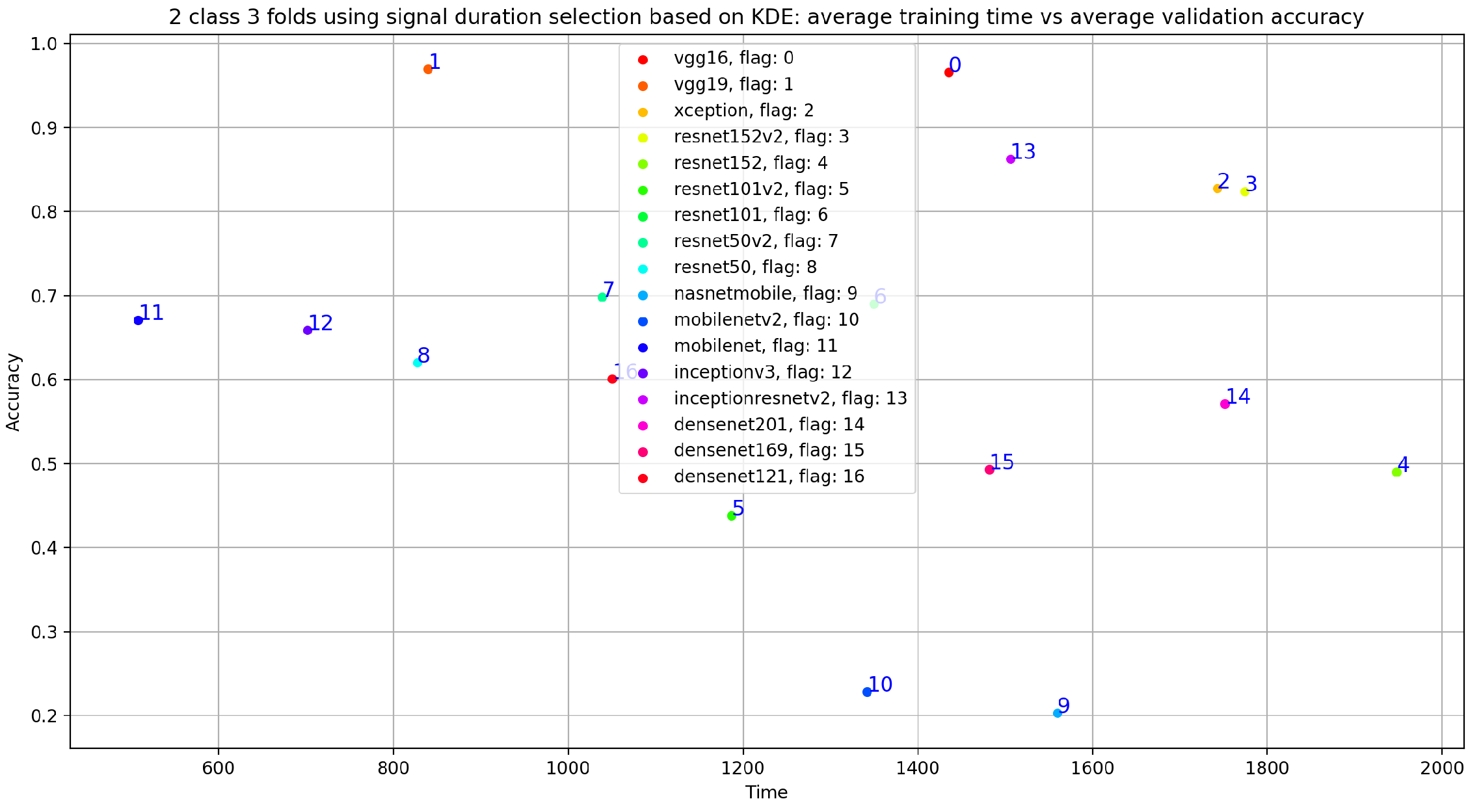
Classification Using Kernel Density Estimation as Data Selection Method for Signal Duration 20 s Normal and 35 s Abnormal
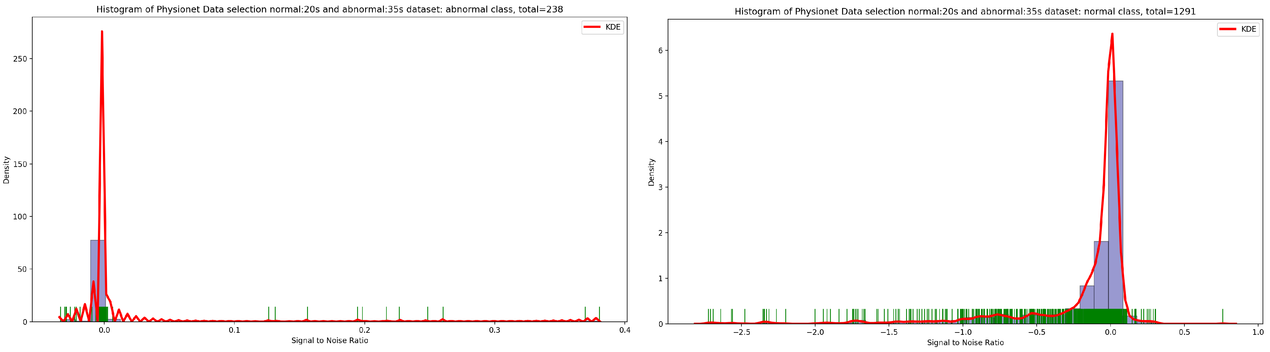
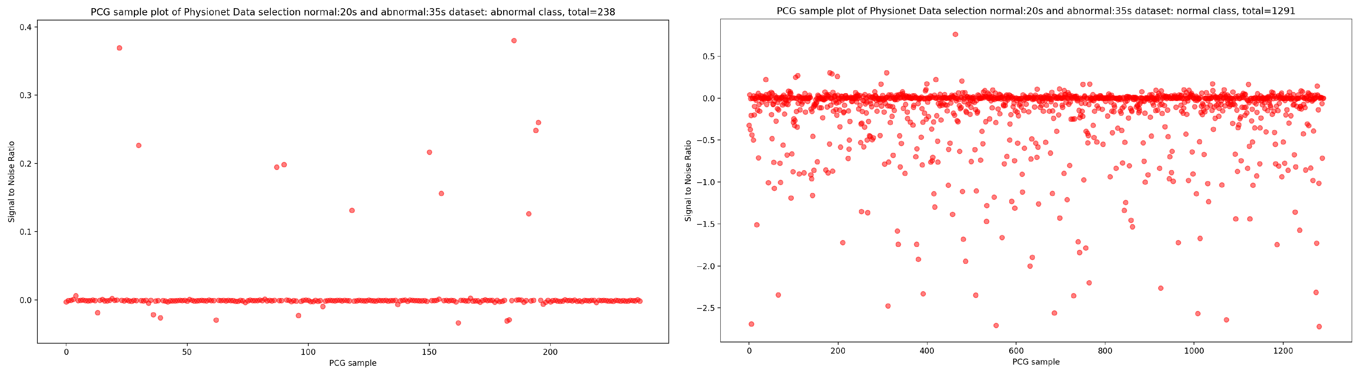
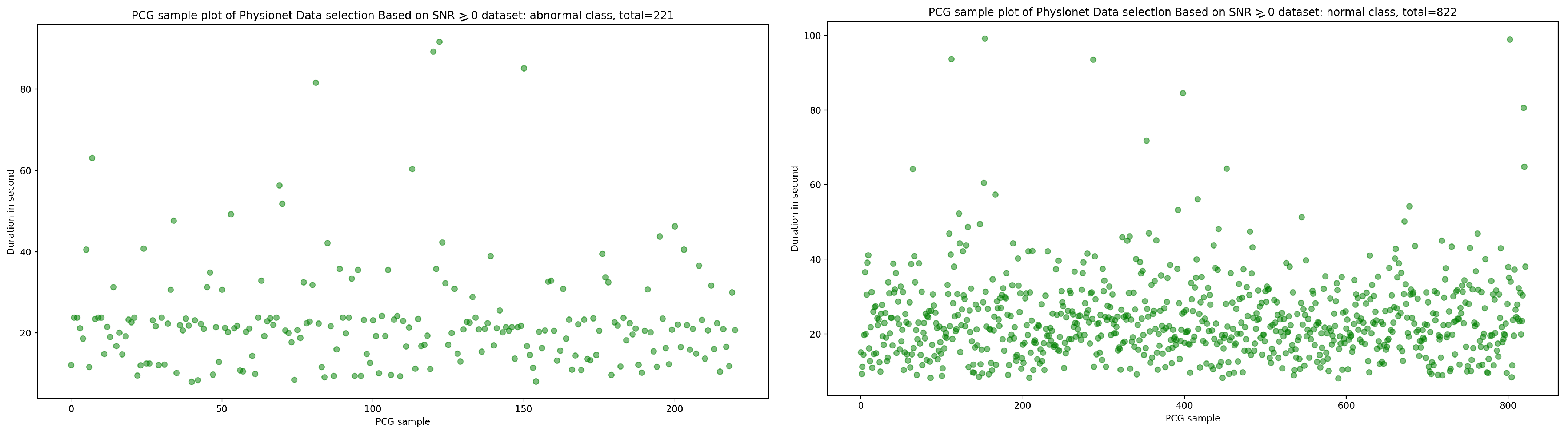
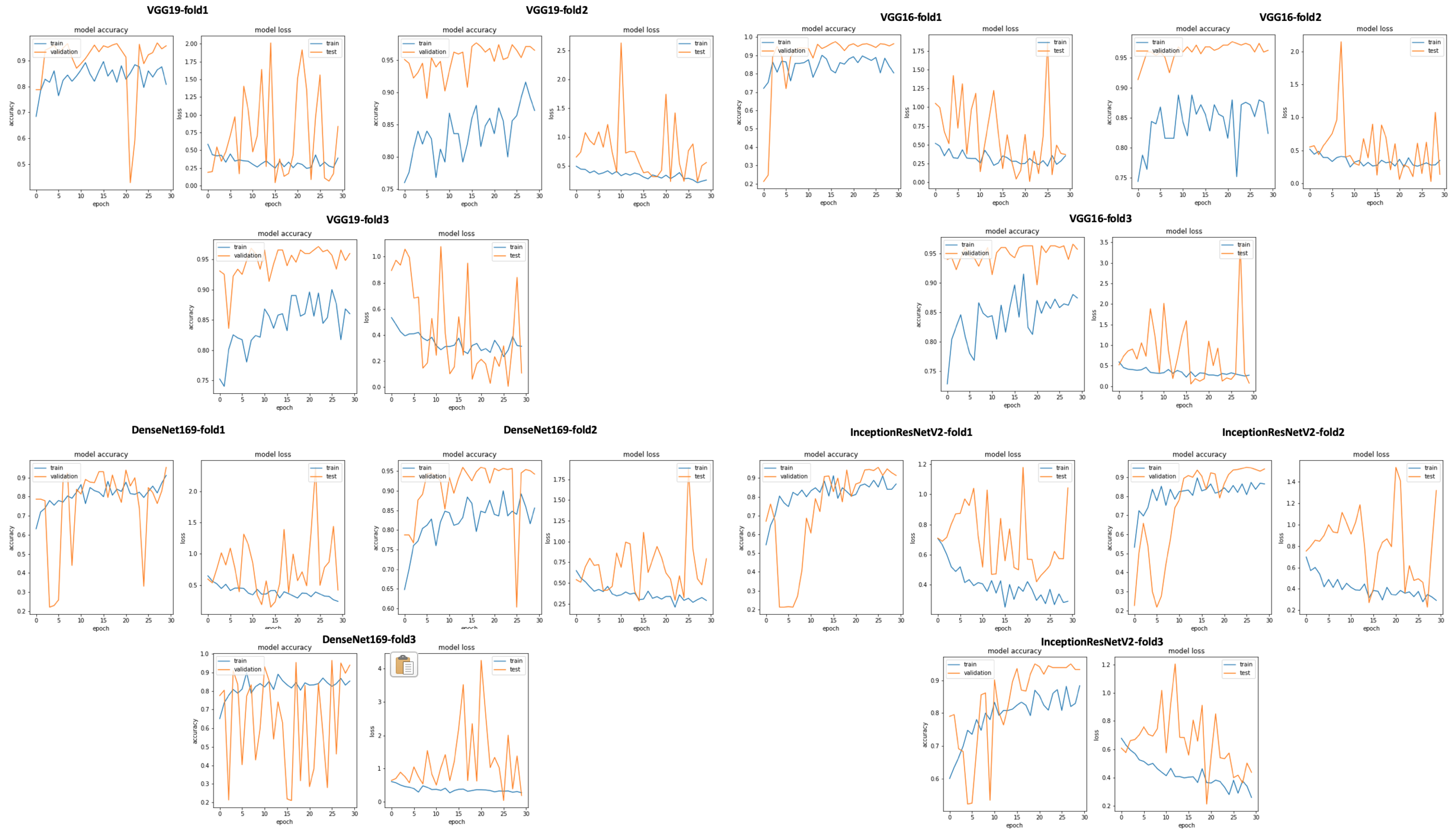
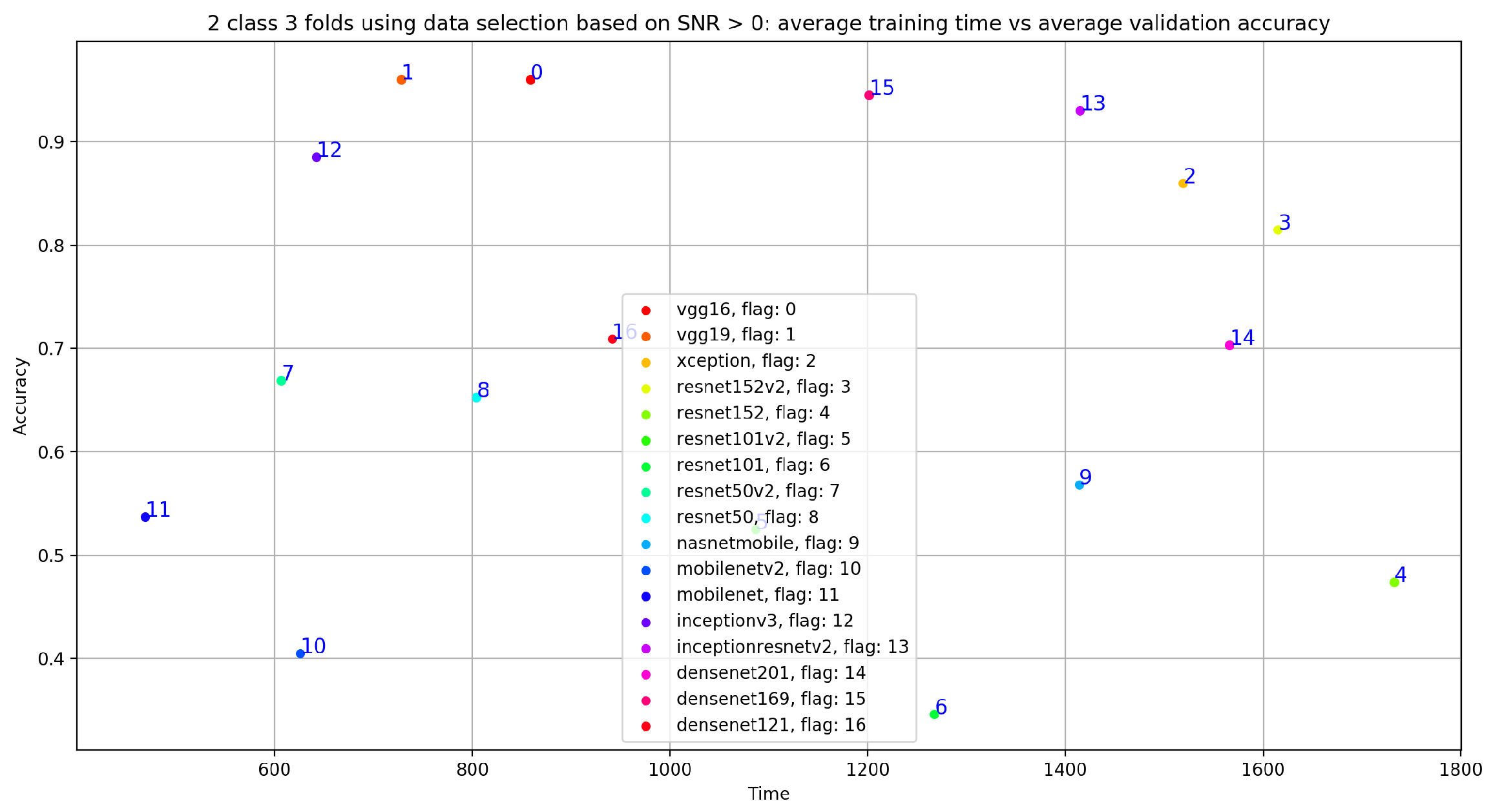
5.2. Classification Using Data Selection Based on Optimal SNR
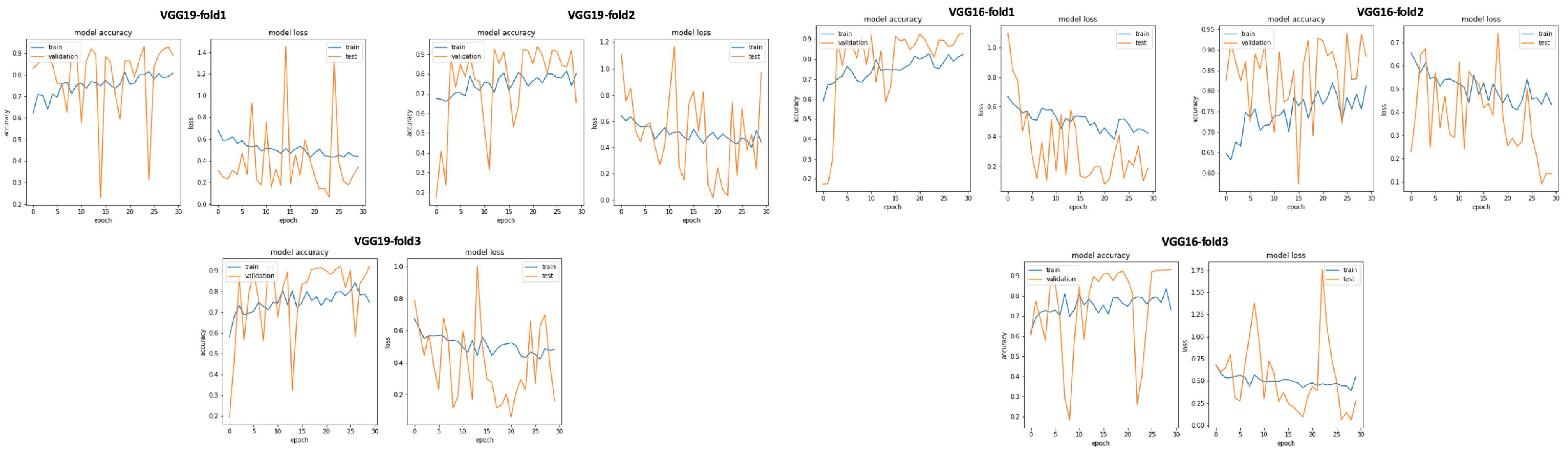
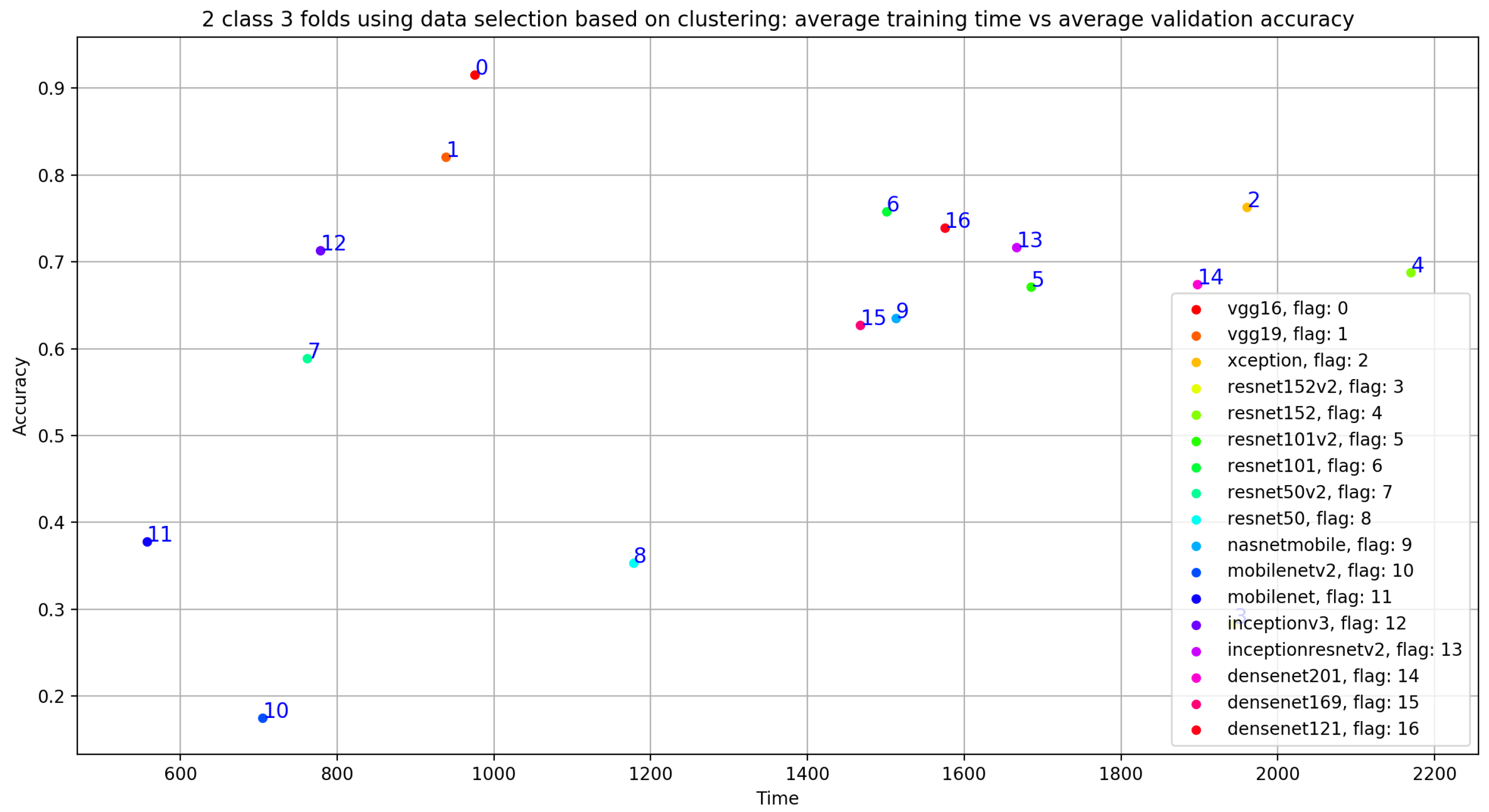
5.2.1. Classification Using Clustering as Data Selection Method
5.2.2. Synthesis
6. Conclusions and Perspectives
Author Contributions
Funding
Institutional Review Board Statement
Informed Consent Statement
Data Availability Statement
Acknowledgments
Conflicts of Interest
References
- World Health Organization. World Health Ranking. 2020. Available online: https://www.who.int/health-topics/cardiovascular-diseases#tab=tab_1 (accessed on 15 February 2021).
- Yang, Z.J.; Liu, J.; Ge, J.P.; Chen, L.; Zhao, Z.G.; Yang, W.Y. Prevalence of Cardiovascular Disease Risk Factor in the Chinese Population: The 2007–2008 China National Diabetes and Metabolic Disorders Study. Eur. Heart J. 2011, 33, 213–220. [Google Scholar] [CrossRef] [PubMed]
- Mangione, S.; Nieman, L.Z. Cardiac Auscultatory Skills of Internal Medicine and Family Practice Trainees: A Comparison of Diagnostic Proficiency. JAMA 1997, 278, 717–722. [Google Scholar] [CrossRef] [PubMed]
- Lam, M.; Lee, T.; Boey, P.; Ng, W.; Hey, H.; Ho, K.; Cheong, P. Factors influencing cardiac auscultation proficiency in physician trainees. Singap. Med. J. 2005, 46, 11–14. [Google Scholar]
- Roelandt, J. The decline of our physical examination skills: Is echocardiography to blame? Eur. Heart J. Cardiovasc. Imaging 2013, 15, 249–252. [Google Scholar] [CrossRef]
- Grzegorczyk, I.; Soliński, M.; Łepek, M.; Perka, A.; Rosiński, J.; Rymko, J.; Stępień, K.; Gierałtowski, J. PCG classification using a neural network approach. In Proceedings of the 2016 Computing in Cardiology Conference (CinC), Vancouver, BC, Canada, 11–14 September 2016; pp. 1129–1132. [Google Scholar]
- Liu, C.; Springer, D.; Li, Q.; Moody, B.; Juan, R.A.; Chorro, F.J.; Castells, F.; Roig, J.M.; Silva, I.; Johnson, A.E.; et al. An open access database for the evaluation of heart sound algorithms. Physiol. Meas. 2016, 37, 2181. [Google Scholar] [CrossRef]
- Nouraei, H.; Nouraei, H.; Rabkin, S.W. Comparison of Unsupervised Machine Learning Approaches for Cluster Analysis to Define Subgroups of Heart Failure with Preserved Ejection Fraction with Different Outcomes. Bioengineering 2022, 9, 175. [Google Scholar] [CrossRef]
- Aruleba, R.T.; Adekiya, T.A.; Ayawei, N.; Obaido, G.; Aruleba, K.; Mienye, I.D.; Aruleba, I.; Ogbuokiri, B. COVID-19 Diagnosis: A Review of Rapid Antigen, RT-PCR and Artificial Intelligence Methods. Bioengineering 2022, 9, 153. [Google Scholar] [CrossRef]
- Elaziz, M.A.; Hosny, K.M.; Salah, A.; Darwish, M.M.; Lu, S.; Sahlol, A.T. New machine learning method for image-based diagnosis of COVID-19. PLoS ONE 2020, 15, e0235187. [Google Scholar] [CrossRef]
- Magar, R.; Yadav, P.; Barati Farimani, A. Potential neutralizing antibodies discovered for novel corona virus using machine learning. Sci. Rep. 2021, 11, 5261. [Google Scholar] [CrossRef]
- Sujath, R.A.A.; Chatterjee, J.M.; Hassanien, A.E. A machine learning forecasting model for COVID-19 pandemic in India. Stoch. Environ. Res. Risk Assess. 2020, 34, 959–972. [Google Scholar] [CrossRef]
- Chintalapudi, N.; Battineni, G.; Hossain, M.A.; Amenta, F. Cascaded Deep Learning Frameworks in Contribution to the Detection of Parkinson’s Disease. Bioengineering 2022, 9, 116. [Google Scholar] [CrossRef] [PubMed]
- Clifford, G.D.; Liu, C.; Moody, B.; Springer, D.; Silva, I.; Li, Q.; Mark, R.G. Classification of normal/abnormal heart sound recordings: The PhysioNet/Computing in Cardiology Challenge 2016. In Proceedings of the 2016 Computing in Cardiology Conference (CinC), Vancouver, BC, Canada, 11–14 September 2016; pp. 609–612. [Google Scholar]
- Nogueira, D.M.; Ferreira, C.A.; Gomes, E.F.; Jorge, A.M. Classifying heart sounds using images of motifs, MFCC and temporal features. J. Med. Syst. 2019, 43, 168. [Google Scholar] [CrossRef] [PubMed]
- Rubin, J.; Abreu, R.; Ganguli, A.; Nelaturi, S.; Matei, I.; Sricharan, K. Recognizing abnormal heart sounds using deep learning. arXiv 2017, arXiv:1707.04642. [Google Scholar]
- Potes, C.; Parvaneh, S.; Rahman, A.; Conroy, B. Ensemble of feature-based and deep learning-based classifiers for detection of abnormal heart sounds. In Proceedings of the 2016 Computing in Cardiology Conference (CinC), Vancouver, BC, Canada, 11–14 September 2016; pp. 621–624. [Google Scholar]
- Tang, H.; Chen, H.; Li, T.; Zhong, M. Classification of normal/abnormal heart sound recordings based on multi-domain features and back propagation neural network. In Proceedings of the 2016 Computing in Cardiology Conference (CinC), Vancouver, BC, Canada, 11–14 September 2016; pp. 593–596. [Google Scholar]
- Kiranyaz, S.; Zabihi, M.; Rad, A.B.; Ince, T.; Hamila, R.; Gabbouj, M. Real-time Phonocardiogram Anomaly Detection by Adaptive 1D Convolutional Neural Networks. Neurocomputing 2020, 411, 291–301. [Google Scholar] [CrossRef]
- Singh, S.A.; Majumder, S. Short unsegmented PCG classification based on ensemble classifier. Turk. J. Electr. Eng. Comput. Sci. 2020, 28, 875–889. [Google Scholar] [CrossRef]
- Krishnan, P.T.; Balasubramanian, P.; Umapathy, S. Automated heart sound classification system from unsegmented phonocardiogram (PCG) using deep neural network. Phys. Eng. Sci. Med. 2020, 43, 505–515. [Google Scholar] [CrossRef]
- Garg, V.; Mathur, A.; Mangla, N.; Rawat, A.S. Heart Rhythm Abnormality Detection from PCG Signal. In Proceedings of the 2019 Twelfth International Conference on Contemporary Computing (IC3), Noida, India, 8–10 August 2019; pp. 1–5. [Google Scholar]
- Alaskar, H.; Alzhrani, N.; Hussain, A.; Almarshed, F. The Implementation of Pretrained AlexNet on PCG Classification. In Proceedings of the International Conference on Intelligent Computing, Nanchang, China, 3–6 August 2019; pp. 784–794. [Google Scholar]
- Khaled, S.; Fakhry, M.; Mubarak, A.S. Classification of PCG Signals Using A Nonlinear Autoregressive Network with Exogenous Inputs (NARX). In Proceedings of the 2020 International Conference on Innovative Trends in Communication and Computer Engineering (ITCE), Aswan, Egypt, 8–9 February 2020; pp. 98–102. [Google Scholar]
- Noman, F.; Ting, C.M.; Salleh, S.H.; Ombao, H. Short-segment heart sound classification using an ensemble of deep convolutional neural networks. In Proceedings of the ICASSP 2019—2019 IEEE International Conference on Acoustics, Speech and Signal Processing (ICASSP), Brighton, UK, 12–17 May 2019; pp. 1318–1322. [Google Scholar]
- Parzen, E. On estimation of a probability density function and mode. Ann. Math. Stat. 1962, 33, 1065–1076. [Google Scholar] [CrossRef]
- Hoult, D.I.; Richards, R. The signal-to-noise ratio of the nuclear magnetic resonance experiment. J. Magn. Reson. (1969) 1976, 24, 71–85. [Google Scholar] [CrossRef]
- McLachlan, G.; Peel, D. Finite Mixture Models; John Wiley & Sons: Hoboken, NJ, USA, 2004. [Google Scholar]
- McLachlan, G.; Krishnan, T. The EM Algorithm and Extensions; John Wiley & Sons: Hoboken, NJ, USA, 2007; Volume 382. [Google Scholar]
- Bishop, C.M. Pattern Recognition and Machine Learning; Springer: Berlin/Heidelberg, Germany, 2006. [Google Scholar]
- Hastie, T.; Tibshirani, R.; Friedman, J.; Franklin, J. The elements of statistical learning: Data mining, inference and prediction. Math. Intell. 2005, 27, 83–85. [Google Scholar]
- Fayek, H.M. Speech Processing for Machine Learning: Filter Banks, Mel Frequency Cepstral Coefficients (MFCCs) and What’s In-Between. 2016. Available online: https://haythamfayek.com/2016/04/21/speech-processing-for-machine-learning.html (accessed on 15 February 2021).
- Dave, N. Feature extraction methods LPC, PLP and MFCC in speech recognition. Int. J. Adv. Res. Eng. Technol. 2013, 1, 1–4. [Google Scholar]
- Han, W.; Chan, C.F.; Choy, C.S.; Pun, K.P. An efficient MFCC extraction method in speech recognition. In Proceedings of the 2006 IEEE International Symposium on Circuits and Systems, Kos, Greece, 21–24 May 2006; p. 4. [Google Scholar]
- Al Marzuqi, H.M.O.; Hussain, S.M.; Frank, A. Device Activation based on Voice Recognition using Mel Frequency Cepstral Coefficients (MFCC’s) Algorithm. Int. Res. J. Eng. Technol. 2019, 6, 4297–4301. [Google Scholar]
- Milletari, F.; Ahmadi, S.A.; Kroll, C.; Plate, A.; Rozanski, V.; Maiostre, J.; Levin, J.; Dietrich, O.; Ertl-Wagner, B.; Bötzel, K.; et al. Hough-CNN: Deep learning for segmentation of deep brain regions in MRI and ultrasound. Comput. Vis. Image Underst. 2017, 164, 92–102. [Google Scholar] [CrossRef]
- Bar, Y.; Diamant, I.; Wolf, L.; Lieberman, S.; Konen, E.; Greenspan, H. Chest pathology detection using deep learning with non-medical training. In Proceedings of the 2015 IEEE 12th iNternational Symposium On Biomedical Imaging (ISBI), Brooklyn, NY, USA, 16–19 April 2015; pp. 294–297. [Google Scholar]
- Yan, L.; Yoshua, B.; Geoffrey, H. Deep learning. Nature 2015, 521, 436–444. [Google Scholar]
- Li, W.; Wu, G.; Du, Q. Transferred deep learning for anomaly detection in hyperspectral imagery. IEEE Geosci. Remote. Sens. Lett. 2017, 14, 597–601. [Google Scholar] [CrossRef]
- LeCun, Y.; Bottou, L.; Bengio, Y.; Haffner, P. Gradient-based learning applied to document recognition. Proc. IEEE 1998, 86, 2278–2324. [Google Scholar] [CrossRef]
- Jiang, H.; Learned-Miller, E. Face detection with the faster R-CNN. In Proceedings of the 2017 12th IEEE International Conference on Automatic Face & Gesture Recognition (FG 2017), Washington, DC, USA, 30 May–3 June 2017; pp. 650–657. [Google Scholar]
- Zhu, C.; Zheng, Y.; Luu, K.; Savvides, M. Cms-rcnn: Contextual multi-scale region-based cnn for unconstrained face detection. In Deep Learning for Biometrics; Springer: Berlin/Heidelberg, Germany, 2017; pp. 57–79. [Google Scholar]
- Li, H.; Lin, Z.; Shen, X.; Brandt, J.; Hua, G. A convolutional neural network cascade for face detection. In Proceedings of the IEEE Conference on Computer Vision and Pattern Recognition, Boston, MA, USA, 7–12 June 2015; pp. 5325–5334. [Google Scholar]
- Niu, X.X.; Suen, C.Y. A novel hybrid CNN—SVM classifier for recognizing handwritten digits. Pattern Recognit. 2012, 45, 1318–1325. [Google Scholar] [CrossRef]
- Matsumoto, T.; Chua, L.O.; Suzuki, H. CNN cloning template: Connected component detector. IEEE Trans. Circuits Syst. 1990, 37, 633–635. [Google Scholar] [CrossRef]
- Wu, C.; Fan, W.; He, Y.; Sun, J.; Naoi, S. Handwritten character recognition by alternately trained relaxation convolutional neural network. In Proceedings of the 2014 14th International Conference on Frontiers in Handwriting Recognition, Crete Island, Greece, 1–4 September 2014; pp. 291–296. [Google Scholar]
- Wang, J.; Yang, Y.; Mao, J.; Huang, Z.; Huang, C.; Xu, W. Cnn-rnn: A unified framework for multi-label image classification. In Proceedings of the IEEE Conference on Computer Vision and Pattern Recognition, Las Vegas, NV, USA, 27–30 June 2016; pp. 2285–2294. [Google Scholar]
- Lee, H.; Kwon, H. Going deeper with contextual CNN for hyperspectral image classification. IEEE Trans. Image Process. 2017, 26, 4843–4855. [Google Scholar] [CrossRef]
- Yu, S.; Jia, S.; Xu, C. Convolutional neural networks for hyperspectral image classification. Neurocomputing 2017, 219, 88–98. [Google Scholar] [CrossRef]
- Tan, C.; Sun, F.; Kong, T.; Zhang, W.; Yang, C.; Liu, C. A survey on deep transfer learning. In Proceedings of the International Conference on Artificial Neural Networks, Rhodes, Greece, 4–7 October 2018; pp. 270–279. [Google Scholar]
- Chollet, F. Xception: Deep learning with depthwise separable convolutions. In Proceedings of the IEEE Conference on Computer Vision and Pattern Recognition, Honolulu, HI, USA, 21–26 June 2017; pp. 1251–1258. [Google Scholar]
- Simonyan, K.; Zisserman, A. Very deep convolutional networks for large-scale image recognition. arXiv 2014, arXiv:1409.1556. [Google Scholar]
- He, K.; Zhang, X.; Ren, S.; Sun, J. Deep residual learning for image recognition. In Proceedings of the IEEE Conference on Computer Vision and Pattern Recognition, Las Vegas, NV, USA, 27–30 June 2016; pp. 770–778. [Google Scholar]
- Zoph, B.; Vasudevan, V.; Shlens, J.; Le, Q.V. Learning transferable architectures for scalable image recognition. In Proceedings of the IEEE Conference on Computer Vision and Pattern Recognition, Salt Lake City, UT, USA, 18–22 June 2018; pp. 8697–8710. [Google Scholar]
- Sandler, M.; Howard, A.; Zhu, M.; Zhmoginov, A.; Chen, L.C. Mobilenetv2: Inverted residuals and linear bottlenecks. In Proceedings of the IEEE Conference on Computer Vision and Pattern Recognition, Salt Lake City, UT, USA, 18–22 June 2018; pp. 4510–4520. [Google Scholar]
- Howard, A.G.; Zhu, M.; Chen, B.; Kalenichenko, D.; Wang, W.; Weyand, T.; Andreetto, M.; Adam, H. Mobilenets: Efficient convolutional neural networks for mobile vision applications. arXiv 2017, arXiv:1704.04861. [Google Scholar]
- Szegedy, C.; Vanhoucke, V.; Ioffe, S.; Shlens, J.; Wojna, Z. Rethinking the inception architecture for computer vision. In Proceedings of the IEEE Conference on Computer Vision and Pattern Recognition, Las Vegas, NV, USA, 27–30 June 2016; pp. 2818–2826. [Google Scholar]
- Szegedy, C.; Ioffe, S.; Vanhoucke, V.; Alemi, A.A. Inception-v4, inception-resnet and the impact of residual connections on learning. In Proceedings of the Thirty-First AAAI Conference on Artificial Intelligence, San Francisco, CA, USA, 4–9 February 2017. [Google Scholar]
- Huang, G.; Liu, Z.; Van Der Maaten, L.; Weinberger, K.Q. Densely connected convolutional networks. In Proceedings of the IEEE Conference on Computer Vision and Pattern Recognition, Honolulu, HI, USA, 21–26 June 2017; pp. 4700–4708. [Google Scholar]
- Dominguez-Morales, J.P.; Jimenez-Fernandez, A.F.; Dominguez-Morales, M.J.; Jimenez-Moreno, G. Deep neural networks for the recognition and classification of heart murmurs using neuromorphic auditory sensors. IEEE Trans. Biomed. Circuits Syst. 2017, 12, 24–34. [Google Scholar] [CrossRef] [PubMed]
- Langley, P.; Murray, A. Heart sound classification from unsegmented phonocardiograms. Physiol. Meas. 2017, 38, 1658. [Google Scholar] [CrossRef] [PubMed]
- Nogueira, D.M.; Ferreira, C.A.; Jorge, A.M. Classifying heart sounds using images of MFCC and temporal features. In Proceedings of the EPIA Conference on Artificial Intelligence, Porto, Portugal, 5–8 September 2017; pp. 186–203. [Google Scholar]
- Ortiz, J.J.G.; Phoo, C.P.; Wiens, J. Heart sound classification based on temporal alignment techniques. In Proceedings of the 2016 Computing in Cardiology Conference (CinC), Vancouver, BC, Canada, 11–14 September 2016; pp. 589–592. [Google Scholar]
- Kay, E.; Agarwal, A. DropConnected neural networks trained on time-frequency and inter-beat features for classifying heart sounds. Physiol. Meas. 2017, 38, 1645. [Google Scholar] [CrossRef] [PubMed]
- Abdollahpur, M.; Ghiasi, S.; Mollakazemi, M.J.; Ghaffari, A. Cycle selection and neuro-voting system for classifying heart sound recordings. In Proceedings of the 2016 Computing in Cardiology Conference (CinC), Vancouver, BC, Canada, 11–14 September 2016; pp. 1–4. [Google Scholar]
- Han, W.; Yang, Z.; Lu, J.; Xie, S. Supervised threshold-based heart sound classification algorithm. Physiol. Meas. 2018, 39, 115011. [Google Scholar] [CrossRef] [PubMed]
- Whitaker, B.M.; Suresha, P.B.; Liu, C.; Clifford, G.D.; Anderson, D.V. Combining sparse coding and time-domain features for heart sound classification. Physiol. Meas. 2017, 38, 1701. [Google Scholar] [CrossRef] [PubMed]
- Tang, H.; Dai, Z.; Jiang, Y.; Li, T.; Liu, C. PCG classification using multidomain features and SVM classifier. Biomed Res. Int. 2018, 2018, 4205027. [Google Scholar] [CrossRef]
- Plesinger, F.; Viscor, I.; Halamek, J.; Jurco, J.; Jurak, P. Heart sounds analysis using probability assessment. Physiol. Meas. 2017, 38, 1685. [Google Scholar] [CrossRef]
- Abdollahpur, M.; Ghaffari, A.; Ghiasi, S.; Mollakazemi, M.J. Detection of pathological heart sounds. Physiol. Meas. 2017, 38, 1616. [Google Scholar] [CrossRef]
- Homsi, M.N.; Warrick, P. Ensemble methods with outliers for phonocardiogram classification. Physiol. Meas. 2017, 38, 1631. [Google Scholar] [CrossRef]
- Singh, S.A.; Majumder, S. Classification of unsegmented heart sound recording using KNN classifier. J. Mech. Med. Biol. 2019, 19, 1950025. [Google Scholar] [CrossRef]


| Model | Citation | Layers | Size | Parameters |
|---|---|---|---|---|
| Xception | [51] | 71 | 85 MB | 44.6 million |
| VGG19 | [52] | 26 | 549 MB | 143.6 million |
| VGG16 | [52] | 23 | 528 MB | 138.3 million |
| ResNet152V2 | [53] | - | 98 MB | 25.6 million |
| ResNet152 | [53] | - | 232 MB | 60.4 million |
| ResNet101V2 | [53] | - | 171 MB | 44.6 million |
| ResNet101 | [53] | 101 | 167 MB | 44.6 million |
| ResNet50V2 | [53] | 98 MB | 25.6 million | |
| ResNet50 | [53] | - | 98 MB | 25.6 million |
| NASNetMobile | [54] | - | 20 MB | 5.3 million |
| MobileNetV2 | [55] | 53 | 13 MB | 3.5 million |
| MobileNet | [56] | 88 | 16 MB | 4.25 million |
| InceptionV3 | [57] | 48 | 89 MB | 23.9 million |
| InceptionResNetV2 | [58] | 164 | 209 MB | 55.9 million |
| DenseNet201 | [59] | 201 | 77 MB | 20 million |
| DenseNet169 | [59] | 169 | 57 MB | 14.3 million |
| DenseNet121 | [59] | 121 | 33 MB | 8.06 million |
| Average | Accuracy | TPR (Sensitivity) | Precision (PPV) | TNR (Specificity) |
|---|---|---|---|---|
| VGG16 | 0.6 | 0.527 | 0.502 | 0.527 |
| VGG19 | 0.854 | 0.860 | 0.794 | 0.860 |
| Xception | 0.783 | 0.797 | 0.714 | 0.797 |
| ResNet152V2 | 0.659 | 0.679 | 0.665 | 0.679 |
| ResNet152 | 0.580 | 0.689 | 0.634 | 0.689 |
| ResNet101V2 | 0.282 | 0.537 | 0.575 | 0.537 |
| ResNet101 | 0.404 | 0.585 | 0.596 | 0.585 |
| ResNet50v2 | 0.792 | 0.702 | 0.702 | 0.702 |
| ResNet50 | 0.538 | 0.624 | 0.638 | 0.624 |
| NasNetMobile | 0.619 | 0.496 | 0.347 | 0.496 |
| MobileNetV2 | 0.435 | 0.476 | 0.460 | 0.476 |
| MobileNet | 0.558 | 0.595 | 0.653 | 0.595 |
| Inceptionv3 | 0.676 | 0.758 | 0.673 | 0.758 |
| InceptionResNetV2 | 0.825 | 0.807 | 0.748 | 0.807 |
| DenseNet201 | 0.576 | 0.657 | 0.658 | 0.657 |
| DenseNet169 | 0.704 | 0.771 | 0.715 | 0.771 |
| DenseNet121 | 0.424 | 0.622 | 0.620 | 0.622 |
| Average | Accuracy | TPR (Sensitivity) | Precision (PPV) | TNR (Specificity) |
|---|---|---|---|---|
| VGG16 | 0.966 | 0.930 | 0.946 | 0.930 |
| VGG19 | 0.970 | 0.946 | 0.944 | 0.946 |
| Xception | 0.828 | 0.877 | 0.732 | 0.877 |
| ResNet152V2 | 0.824 | 0.873 | 0.730 | 0.873 |
| ResNet152 | 0.490 | 0.667 | 0.640 | 0.667 |
| ResNet101V2 | 0.438 | 0.665 | 0.422 | 0.665 |
| ResNet101 | 0.690 | 0.592 | 0.812 | 0.592 |
| ResNet50v2 | 0.698 | 0.736 | 0.728 | 0.736 |
| ResNet50 | 0.620 | 0.763 | 0.685 | 0.763 |
| NasNetMobile | 0.203 | 0.489 | 0.350 | 0.489 |
| MobileNetV2 | 0.228 | 0.497 | 0.526 | 0.497 |
| MobileNet | 0.671 | 0.679 | 0.673 | 0.679 |
| Inceptionv3 | 0.659 | 0.791 | 0.686 | 0.791 |
| InceptionResNetV2 | 0.863 | 0.908 | 0.765 | 0.908 |
| DenseNet201 | 0.571 | 0.725 | 0.719 | 0.725 |
| DenseNet169 | 0.493 | 0.675 | 0.606 | 0.675 |
| DenseNet121 | 0.601 | 0.734 | 0.714 | 0.734 |
| Average | Accuracy | TPR (Sensitivity) | Precision (PPV) | TNR (Specificity) |
|---|---|---|---|---|
| VGG16 | 0.668 | 0.747 | 0.703 | 0.747 |
| VGG19 | 0.870 | 0.851 | 0.801 | 0.851 |
| Xception | 0.702 | 0.781 | 0.689 | 0.781 |
| ResNet152V2 | 0.501 | 0.669 | 0.636 | 0.669 |
| ResNet152 | 0.785 | 0.677 | 0.687 | 0.677 |
| ResNet101V2 | 0.457 | 0.628 | 0.606 | 0.628 |
| ResNet101 | 0.600 | 0.616 | 0.674 | 0.616 |
| ResNet50v2 | 0.433 | 0.626 | 0.611 | 0.626 |
| ResNet50 | 0.473 | 0.581 | 0.636 | 0.581 |
| NasNetMobile | 0.451 | 0.494 | 0.329 | 0.494 |
| MobileNetV2 | 0.576 | 0.535 | 0.541 | 0.535 |
| MobileNet | 0.562 | 0.680 | 0.657 | 0.680 |
| Inceptionv3 | 0.751 | 0.740 | 0.729 | 0.740 |
| InceptionResNetV2 | 0.667 | 0.687 | 0.687 | 0.687 |
| DenseNet201 | 0.694 | 0.744 | 0.713 | 0.744 |
| DenseNet169 | 0.609 | 0.703 | 0.699 | 0.703 |
| DenseNet121 | 0.495 | 0.637 | 0.621 | 0.637 |
| Average | Accuracy | Sensitivity | Precision | Specificity |
|---|---|---|---|---|
| VGG16 | 0.960 | 0.938 | 0.944 | 0.938 |
| VGG19 | 0.960 | 0.943 | 0.940 | 0.943 |
| Xception | 0.860 | 0.895 | 0.807 | 0.895 |
| ResNet152V2 | 0.815 | 0.845 | 0.790 | 0.845 |
| ResNet152 | 0.474 | 0.660 | 0.665 | 0.660 |
| ResNet101V2 | 0.525 | 0.687 | 0.561 | 0.687 |
| ResNet101 | 0.346 | 0.581 | 0.611 | 0.581 |
| ResNet50v2 | 0.669 | 0.773 | 0.745 | 0.773 |
| ResNet50 | 0.653 | 0.746 | 0.566 | 0.746 |
| NasNetMobile | 0.568 | 0.492 | 0.344 | 0.492 |
| MobileNetV2 | 0.405 | 0.561 | 0.521 | 0.561 |
| MobileNet | 0.537 | 0.696 | 0.712 | 0.696 |
| Inceptionv3 | 0.885 | 0.893 | 0.855 | 0.893 |
| InceptionResNetV2 | 0.930 | 0.939 | 0.880 | 0.939 |
| DenseNet201 | 0.703 | 0.789 | 0.612 | 0.789 |
| DenseNet169 | 0.945 | 0.938 | 0.907 | 0.938 |
| DenseNet121 | 0.709 | 0.800 | 0.810 | 0.800 |
| Average | Accuracy | TPR (Sensitivity) | Precision (PPV) | TNR (Specificity) |
|---|---|---|---|---|
| VGG16 | 0.915 | 0.873 | 0.860 | 0.873 |
| VGG19 | 0.821 | 0.808 | 0.787 | 0.808 |
| Xception | 0.763 | 0.795 | 0.690 | 0.795 |
| ResNet152V2 | 0.283 | 0.561 | 0.590 | 0.561 |
| ResNet152 | 0.688 | 0.712 | 0.728 | 0.712 |
| ResNet101V2 | 0.671 | 0.702 | 0.674 | 0.702 |
| ResNet101 | 0.758 | 0.765 | 0.682 | 0.765 |
| ResNet50v2 | 0.589 | 0.666 | 0.633 | 0.666 |
| ResNet50 | 0.353 | 0.576 | 0.396 | 0.576 |
| NasNetMobile | 0.635 | 0.498 | 0.561 | 0.498 |
| MobileNetV2 | 0.175 | 0.500 | 0.195 | 0.500 |
| MobileNet | 0.378 | 0.606 | 0.422 | 0.606 |
| Inceptionv3 | 0.713 | 0.773 | 0.668 | 0.773 |
| InceptionResNetV2 | 0.717 | 0.717 | 0.761 | 0.717 |
| DenseNet201 | 0.674 | 0.746 | 0.672 | 0.746 |
| DenseNet169 | 0.627 | 0.758 | 0.656 | 0.758 |
| DenseNet121 | 0.739 | 0.683 | 0.762 | 0.683 |
| Average | Accuracy | TPR (Sensitivity) | Precision (PPV) | TNR (Specificity) |
|---|---|---|---|---|
| our approach | 0.970 | 0.946 | 0.944 | 0.946 |
| [62] | 0.8697 | 0.964 | - | 0.726 |
| [17] | - | 0.942 | - | 0.778 |
| [63] | 0.824 | - | - | - |
| [18] | - | 0.8095 | - | 0.839 |
| [16] | - | 0.84 | - | 0.957 |
| [64] | 0.852 | - | - | - |
| [65] | - | 0.885 | - | 0.921 |
| [20] | 0.879 | 0.885 | - | 0.878 |
| [60] | 0.97 | 0.932 | - | 0.951 |
| [66] | 0.915 | 0.983 | 0.846 | |
| [67] | 0.892 | 0.90 | - | 0.884 |
| [68] | 0.88 | 0.88 | - | 0.87 |
| [69] | 0.85 | 0.89 | - | 0.816 |
| [70] | 0.826 | 0.769 | - | 0.883 |
| [71] | 0.801 | 0.796 | - | 0.806 |
| [72] | 0.9 | 0.93 | - | 0.9 |
| [61] | 0.79 | 0.77 | - | 0.8 |
Disclaimer/Publisher’s Note: The statements, opinions and data contained in all publications are solely those of the individual author(s) and contributor(s) and not of MDPI and/or the editor(s). MDPI and/or the editor(s) disclaim responsibility for any injury to people or property resulting from any ideas, methods, instructions or products referred to in the content. |
© 2023 by the authors. Licensee MDPI, Basel, Switzerland. This article is an open access article distributed under the terms and conditions of the Creative Commons Attribution (CC BY) license (https://creativecommons.org/licenses/by/4.0/).
Share and Cite
Barnawi, A.; Boulares, M.; Somai, R. Simple and Powerful PCG Classification Method Based on Selection and Transfer Learning for Precision Medicine Application. Bioengineering 2023, 10, 294. https://doi.org/10.3390/bioengineering10030294
Barnawi A, Boulares M, Somai R. Simple and Powerful PCG Classification Method Based on Selection and Transfer Learning for Precision Medicine Application. Bioengineering. 2023; 10(3):294. https://doi.org/10.3390/bioengineering10030294
Chicago/Turabian StyleBarnawi, Ahmed, Mehrez Boulares, and Rim Somai. 2023. "Simple and Powerful PCG Classification Method Based on Selection and Transfer Learning for Precision Medicine Application" Bioengineering 10, no. 3: 294. https://doi.org/10.3390/bioengineering10030294
APA StyleBarnawi, A., Boulares, M., & Somai, R. (2023). Simple and Powerful PCG Classification Method Based on Selection and Transfer Learning for Precision Medicine Application. Bioengineering, 10(3), 294. https://doi.org/10.3390/bioengineering10030294