

Non-Invasive Electroanatomical Mapping: A State-Space Approach for Myocardial Current Density Estimation

 , , ,
, , , 
Abstract
:1. Introduction
1.1. Motivation
1.2. State of the Art
1.3. Contributions
2. Methods
2.1. Overview
2.2. Forward Model
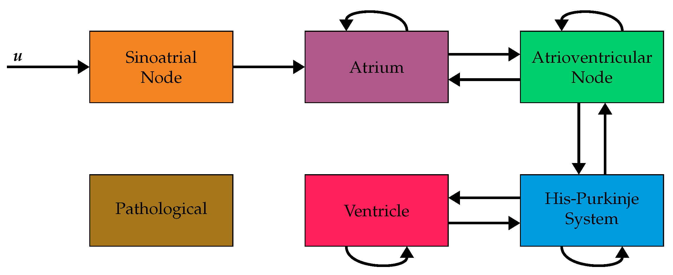
2.3. System Model
2.4. Model Initialization
- The iteration time is set to 0 ms.
- For all voxels with an activation time equal to the iteration time the following steps are carried out.
- (a)
- Identify all neighboring voxels , that have not been connected yet.
- (b)
- Discard all neighbors with incompatible voxel types (cf. Figure 2).
- (c)
- Calculate the current direction in according to the following equation, where is the position of the voxel and it the position of the voxel :
- (d)
- Calculate the gains between two voxels and according to the following equation:The indices i and o are dropped for better readability and the indices are used to index the three by three matrix .
- (e)
- Calculate the activation time of the voxel as .
- Set the iteration time to the smallest activation time that is bigger than the current iteration time .
2.5. State Estimation
2.6. Model Refinement
3. Simulations
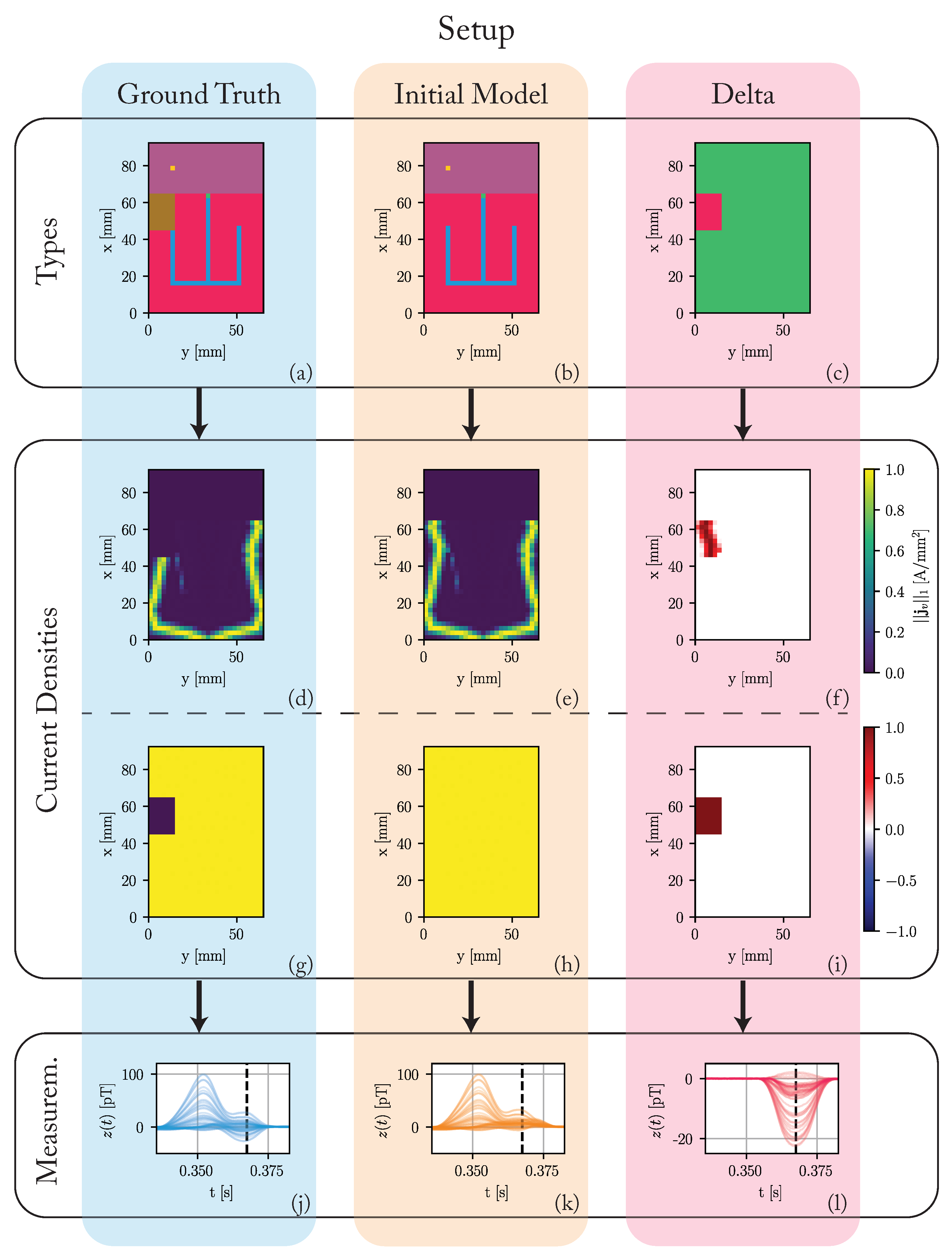
3.1. Setup
3.2. Results
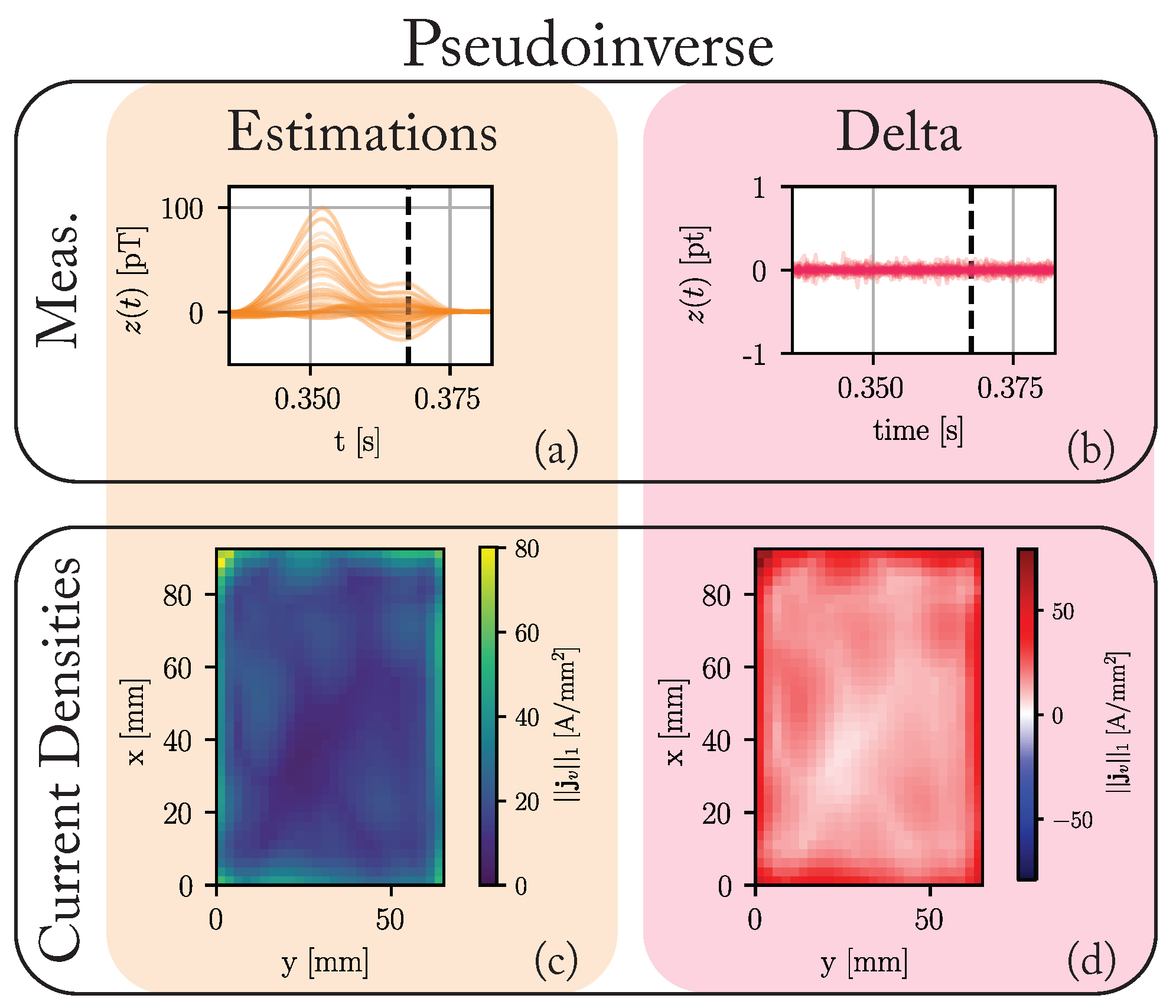
3.2.1. Pseudoinverse
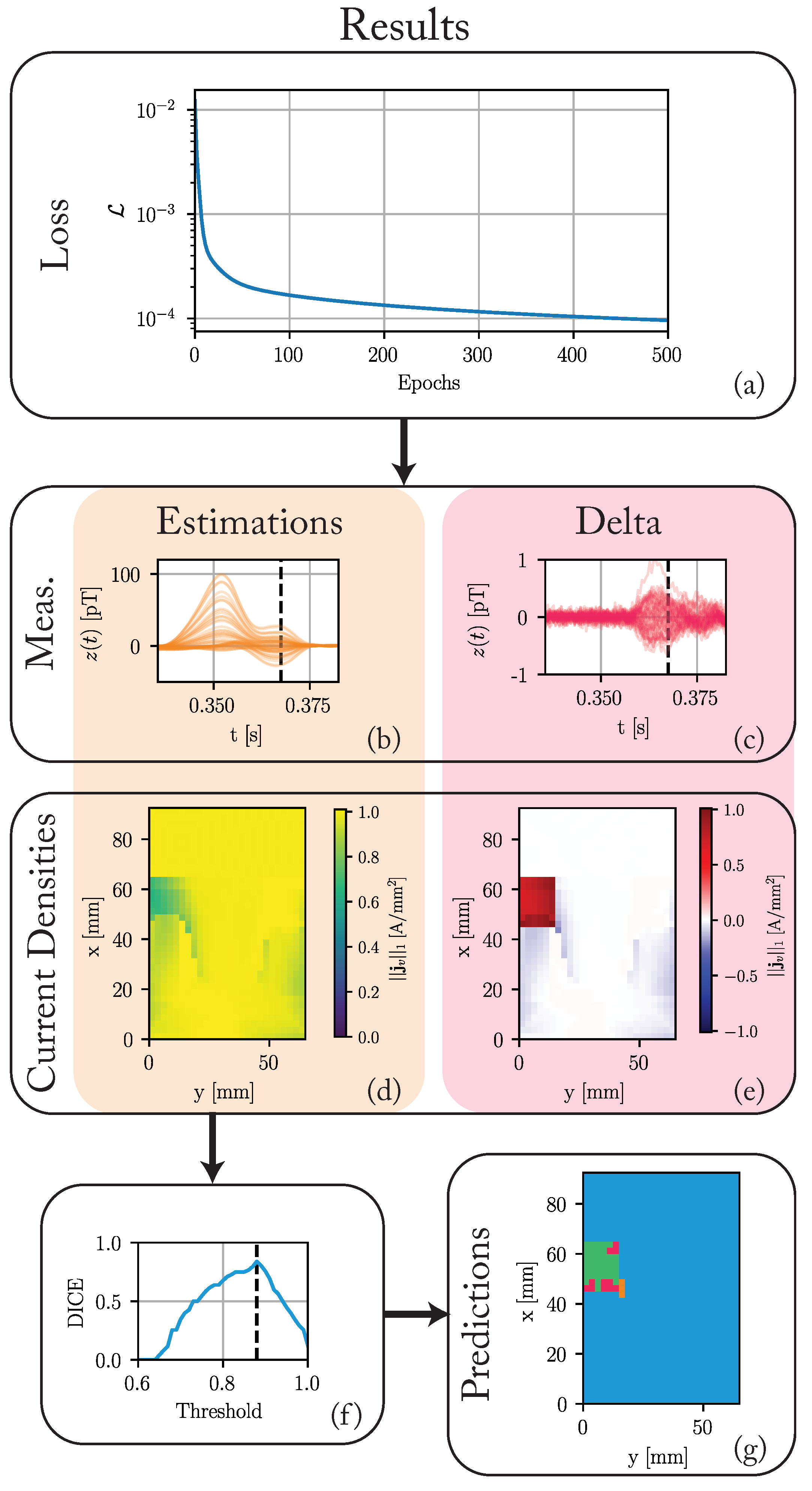
3.2.2. State-Space Approach
3.3. Discussion
4. Conclusions
Author Contributions
Funding
Institutional Review Board Statement
Informed Consent Statement
Data Availability Statement
Conflicts of Interest
Abbreviations
| AV | Atrioventricular |
| EEG | Electroencephalography |
| ECG | Electrocardiography |
| HPS | HIS-Purkinje system |
| MCG | Magnetocardiography |
| MRI | Magnetic resonance imaging |
| SA | Sinoatrial |
| SBRT | Stereotactic Body Radiation Therapy |
| SQUID | Superconducting quantum interference device |
References
- Sidney, S.; Quesenberry, C.P.; Jaffe, M.G.; Sorel, M.; Nguyen-Huynh, M.N.; Kushi, L.H.; Go, A.S.; Rana, J.S. Recent Trends in Cardiovascular Mortality in the United States and Public Health Goals. JAMA Cardiol. 2016, 1, 594. [Google Scholar] [CrossRef]
- Wang, L.; Zhang, H.; Wong, K.; Liu, H.; Shi, P. Noninvasive Imaging of 3D Cardiac Electrophysiology. In Proceedings of the 2007 4th IEEE International Symposium on Biomedical Imaging: From Nano to Macro, Arlington, VA, USA, 12–15 April 2007; pp. 632–635. [Google Scholar] [CrossRef]
- Malkin, R.A.; Kramer, N.; Schnitz, B.; Gopalakrishnan, M.; Curry, A.L. Advances in electrical and mechanical cardiac mapping. Physiol. Meas. 2005, 26, R1–R14. [Google Scholar] [CrossRef]
- Benedict, S.H.; Yenice, K.M.; Followill, D.; Galvin, J.M.; Hinson, W.; Kavanagh, B.; Keall, P.; Lovelock, M.; Meeks, S.; Papiez, L.; et al. Stereotactic body radiation therapy: The report of AAPM Task Group 101. Med. Phys. 2010, 37, 4078–4101. [Google Scholar] [CrossRef]
- Pereira, H.; Niederer, S.; Rinaldi, C.A. Electrocardiographic imaging for cardiac arrhythmias and resynchronization therapy. EP Eur. 2020, 22, 1447–1462. [Google Scholar] [CrossRef] [PubMed]
- Loo, B.W.; Soltys, S.G.; Wang, L.; Lo, A.; Fahimian, B.P.; Iagaru, A.; Norton, L.; Shan, X.; Gardner, E.; Fogarty, T.; et al. Stereotactic Ablative Radiotherapy for the Treatment of Refractory Cardiac Ventricular Arrhythmia. Circ. Arrhythmia Electrophysiol. 2015, 8, 748–750. [Google Scholar] [CrossRef]
- Bourier, F.; Fahrig, R.; Wang, P.; Santangeli, P.; Kurzidim, K.; Strobel, N.; Moore, T.; Hinkel, C.; Al-Ahmad, A. Accuracy Assessment of Catheter Guidance Technology in Electrophysiology Procedures: A Comparison of a New 3D-Based Fluoroscopy Navigation System to Current Electroanatomic Mapping Systems. J. Cardiovasc. Electrophysiol. 2014, 25, 74–83. [Google Scholar] [CrossRef]
- Fenici, R.; Brisinda, D.; Meloni, A.M. Clinical application of magnetocardiography. Expert Rev. Mol. Diagn. 2005, 5, 291–313. [Google Scholar] [CrossRef] [PubMed]
- Chen, K.W.; Bear, L.; Lin, C.W. Solving Inverse Electrocardiographic Mapping Using Machine Learning and Deep Learning Frameworks. Sensors 2022, 22, 2331. [Google Scholar] [CrossRef] [PubMed]
- Pesola, K.; Nenonen, J.; Fenici, R.; Lötjönen, J.; Mäkijärvi, M.; Fenici, P.; Korhonen, P.; Lauerma, K.; Valkonen, M.; Toivonen, L.; et al. Bioelectromagnetic localization of a pacing catheter in the heart. Phys. Med. Biol. 1999, 44, 2565–2578. [Google Scholar] [CrossRef] [PubMed]
- Hu, Z.; Ye, K.; Bai, M.; Yang, Z.; Lin, Q. Solving the magnetocardiography forward problem in a realistic three-dimensional heart-torso model. IEEE Access 2021, 9, 107095–107103. [Google Scholar] [CrossRef]
- Haberkorn, W.; Steinhoff, U.; Burghoff, M.; Kosch, O.; Morguet, A.; Koch, H. Pseudo current density maps of electrophysiological heart, nerve or brain function and their physical basis. BioMagn. Res. Technol. 2006, 4, 5. [Google Scholar] [CrossRef]
- Smith, F.E.; Langley, P.; van Leeuwen, P.; Hailer, B.; Trahms, L.; Steinhoff, U.; Bourke, J.P.; Murray, A. Comparison of magnetocardiography and electrocardiography: A study of automatic measurement of dispersion of ventricular repolarization. EP Eur. 2006, 8, 887–893. [Google Scholar] [CrossRef]
- Lant, J.; Stroink, G.; ten Voorde, B.; Horacek, B.; Montague, T.J. Complementary nature of electrocardiographic and magnetocardiographic data in patients with ischemic heart disease. J. Electrocardiol. 1990, 23, 315–322. [Google Scholar] [CrossRef]
- Gillette, K.; Gsell, M.A.F.; Strocchi, M.; Grandits, T.; Neic, A.; Manninger, M.; Scherr, D.; Roney, C.H.; Prassl, A.J.; Augustin, C.M.; et al. A personalized real-time virtual model of whole heart electrophysiology. Front. Physiol. 2022, 13, 907190. [Google Scholar] [CrossRef] [PubMed]
- Kléber, A.G.; Rudy, Y. Basic Mechanisms of Cardiac Impulse Propagation and Associated Arrhythmias. Physiol. Rev. 2004, 84, 431–488. [Google Scholar] [CrossRef] [PubMed]
- Meijler, F.L.; Janse, M.J. Morphology and electrophysiology of the mammalian atrioventricular node. Physiol. Rev. 1988, 68, 608–647. [Google Scholar] [CrossRef] [PubMed]
- Kassebaum, D.G.; Van Dyke, A.R. Electrophysiological Effects of Isoproterenol on Purkinje Fibers of the Heart. Circ. Res. 1966, 19, 940–946. [Google Scholar] [CrossRef] [PubMed]
- Thiran, J.P. Recursive digital filters with maximally flat group delay. IEEE Trans. Circuit Theory 1971, 18, 659–664. [Google Scholar] [CrossRef]
- Clerx, M.; Collins, P.; de Lange, E.; Volders, P.G. Myokit: A simple interface to cardiac cellular electrophysiology. Prog. Biophys. Mol. Biol. 2016, 120, 100–114. [Google Scholar] [CrossRef] [PubMed]
- O’Hara, T.; Virág, L.; Varró, A.; Rudy, Y. Simulation of the Undiseased Human Cardiac Ventricular Action Potential: Model Formulation and Experimental Validation. PLoS Comput. Biol. 2011, 7, e1002061. [Google Scholar] [CrossRef]
- Taggart, P.; Sutton, P.M.; Opthof, T.; Coronel, R.; Trimlett, R.; Pugsley, W.; Kallis, P. Inhomogeneous Transmural Conduction During Early Ischaemia in Patients with Coronary Artery Disease. J. Mol. Cell. Cardiol. 2000, 32, 621–630. [Google Scholar] [CrossRef] [PubMed]
- Nagel, C.; Schuler, S.; Dössel, O.; Loewe, A. A bi-atrial statistical shape model for large-scale in silico studies of human atria: Model development and application to ECG simulations. Med. Image Anal. 2021, 74, 102210. [Google Scholar] [CrossRef]
- Engelhardt, E.; Elzenheimer, E.; Hoffmann, J.; Schmidt, T.; Zaman, A.; Frey, N.; Schmidt, G. A Concept for Myocardial Current Density Estimation with Magnetoelectric Sensors. Curr. Dir. Biomed. Eng. 2023, 9, 89–92. [Google Scholar] [CrossRef]
- Kucera, J.P.; Kléber, A.G.; Rohr, S. Slow Conduction in Cardiac Tissue, II: Effects of Branching Tissue Geometry. Circ. Res. 1998, 83, 795–805. [Google Scholar] [CrossRef]
- Kucera, J.P.; Rudy, Y. Mechanistic Insights Into Very Slow Conduction in Branching Cardiac Tissue: A Model Study. Circ. Res. 2001, 89, 799–806. [Google Scholar] [CrossRef]
- Haykin, S.S. Adaptive Filter Theory, 4th ed.; international ed.; Prentice Hall informations and system sciences series; Prentice Hall: Upper Saddle River, NJ, USA, 2002. [Google Scholar]
- Cronin, E.M.; Bogun, F.M.; Maury, P.; Peichl, P.; Chen, M.; Namboodiri, N.; Aguinaga, L.; Leite, L.R.; Al-Khatib, S.M.; Anter, E.; et al. 2019 HRS/EHRA/APHRS/LAHRS expert consensus statement on catheter ablation of ventricular arrhythmias. J. Interv. Card. Electrophysiol. 2020, 59, 145–298. [Google Scholar] [CrossRef]
- Elzenheimer, E.; Bald, C.; Engelhardt, E.; Hoffmann, J.; Hayes, P.; Arbustini, J.; Bahr, A.; Quandt, E.; Höft, M.; Schmidt, G. Quantitative Evaluation for Magnetoelectric Sensor Systems in Biomagnetic Diagnostics. Sensors 2022, 22, 1018. [Google Scholar] [CrossRef]
- Elzenheimer, E.; Hayes, P.; Thormahlen, L.; Engelhardt, E.; Zaman, A.; Quandt, E.; Frey, N.; Hoft, M.; Schmidt, G. Investigation of Converse Magnetoelectric Thin-Film Sensors for Magnetocardiography. IEEE Sens. J. 2023, 23, 5660–5669. [Google Scholar] [CrossRef]
- Reermann, J.; Elzenheimer, E.; Schmidt, G. Real-Time Biomagnetic Signal Processing for Uncooled Magnetometers in Cardiology. IEEE Sens. J. 2019, 19, 4237–4249. [Google Scholar] [CrossRef]
- Gillette, K.; Gsell, M.A.; Prassl, A.J.; Karabelas, E.; Reiter, U.; Reiter, G.; Grandits, T.; Payer, C.; Štern, D.; Urschler, M.; et al. A Framework for the generation of digital twins of cardiac electrophysiology from clinical 12-leads ECGs. Med. Image Anal. 2021, 71, 102080. [Google Scholar] [CrossRef] [PubMed]
- Bruns, S.; Wolterink, J.M.; van den Boogert, T.P.; Runge, J.H.; Bouma, B.J.; Henriques, J.P.; Baan, J.; Viergever, M.A.; Planken, R.N.; Išgum, I. Deep learning-based whole-heart segmentation in 4D contrast-enhanced cardiac CT. Comput. Biol. Med. 2022, 142, 105191. [Google Scholar] [CrossRef] [PubMed]
- Hoffmann, J.; Bald, C.; Schmidt, T.; Boueke, M.; Engelhardt, E.; Krüger, K.; Elzenheimer, E.; Hansen, C.; Maetzler, W.; Schmidt, G. Designing and Validating Magnetic Motion Sensing Approaches with a Real-time Simulation Pipeline. Curr. Dir. Biomed. Eng. 2023, 9, 455–458. [Google Scholar] [CrossRef]
- Brisinda, D.; Fenici, P.; Fenici, R. Clinical magnetocardiography: The unshielded bet—past, present, and future. Front. Cardiovasc. Med. 2023, 10, 1232882. [Google Scholar] [CrossRef] [PubMed]

Disclaimer/Publisher’s Note: The statements, opinions and data contained in all publications are solely those of the individual author(s) and contributor(s) and not of MDPI and/or the editor(s). MDPI and/or the editor(s) disclaim responsibility for any injury to people or property resulting from any ideas, methods, instructions or products referred to in the content. |
© 2023 by the authors. Licensee MDPI, Basel, Switzerland. This article is an open access article distributed under the terms and conditions of the Creative Commons Attribution (CC BY) license (https://creativecommons.org/licenses/by/4.0/).
Share and Cite
Engelhardt, E.; Elzenheimer, E.; Hoffmann, J.; Meledeth, C.; Frey, N.; Schmidt, G. Non-Invasive Electroanatomical Mapping: A State-Space Approach for Myocardial Current Density Estimation. Bioengineering 2023, 10, 1432. https://doi.org/10.3390/bioengineering10121432
Engelhardt E, Elzenheimer E, Hoffmann J, Meledeth C, Frey N, Schmidt G. Non-Invasive Electroanatomical Mapping: A State-Space Approach for Myocardial Current Density Estimation. Bioengineering. 2023; 10(12):1432. https://doi.org/10.3390/bioengineering10121432
Chicago/Turabian StyleEngelhardt, Erik, Eric Elzenheimer, Johannes Hoffmann, Christy Meledeth, Norbert Frey, and Gerhard Schmidt. 2023. "Non-Invasive Electroanatomical Mapping: A State-Space Approach for Myocardial Current Density Estimation" Bioengineering 10, no. 12: 1432. https://doi.org/10.3390/bioengineering10121432
APA StyleEngelhardt, E., Elzenheimer, E., Hoffmann, J., Meledeth, C., Frey, N., & Schmidt, G. (2023). Non-Invasive Electroanatomical Mapping: A State-Space Approach for Myocardial Current Density Estimation. Bioengineering, 10(12), 1432. https://doi.org/10.3390/bioengineering10121432