

Anthropomorphic Characterization of Ankle Joint


Abstract
:1. Introduction
2. Materials and Methods
2.1. Reference Cardinal System
2.2. Morphometric Evaluation
2.3. Statistical Analyses
3. Results
4. Discussion
5. Conclusions
Supplementary Materials
Author Contributions
Funding
Institutional Review Board Statement
Informed Consent Statement
Data Availability Statement
Acknowledgments
Conflicts of Interest
Appendix A

| All Subjects (n = 22) | Female (n = 12) | Male (n = 10) | t-Test | Wilcoxon | Group 1 (n = 6) | Group 2 (n = 9) | Group 3 (n = 7) | Group 1–2 t-Test | Group 1–2 Wilcoxon | Group 1–3 t-Test | Group 1–3 Wilcoxon | Group 2–3 t-Test | Group 2–3 Wilcoxon | CT (n = 8) | MRI (n = 14) | t-Test | Wilcoxon | |||||||||
|---|---|---|---|---|---|---|---|---|---|---|---|---|---|---|---|---|---|---|---|---|---|---|---|---|---|---|
| Parameter | Mean | SD | Mean | SD | Mean | SD | p-Value | p-Value | Mean | SD | Mean | SD | Mean | SD | p-Value | p-Value | p-Value | p-Value | p-Value | p-Value | Mean | SD | Mean | SD | p-Value | p-Value |
| Age | 44 | 17 | 41 | 19 | 47 | 13 | - | 0.1 | 23 | 6 | 46 | 3 | 60 | 12 | - | 0.002 * | - | 0.003 * | - | 0.001 * | 38 | 24 | 47 | 10 | - | 0.1 |
| TiAL medial | 23 | 6 | 22 | 6 | 25 | 7 | 0.2 | - | 18 | 4 | 26 | 7 | 24 | 4 | 0.01 * | - | 0.1 | - | 0.5 | - | 25 | 10 | 23 | 3 | 0.5 | - |
| TiAL middle | 26 | 6 | 24 | 5 | 29 | 6 | 0.05 * | - | 22 | 5 | 29 | 7 | 25 | 3 | 0.01 * | - | 0.3 | - | 0.1 | - | 28 | 10 | 25 | 3 | 0.4 | - |
| TiAL lateral | 24 | 7 | 23 | 6 | 26 | 6 | 0.2 | - | 19 | 4 | 27 | 6 | 24 | 7 | 0.02 * | - | 0.1 | - | 0.4 | - | 27 | 10 | 23 | 4 | 0.3 | - |
| SRTi medial | 26 | 9 | 24 | 7 | 29 | 11 | - | 0.3 | 23 | 6 | 31 | 12 | 23 | 6 | - | 0.2 | - | 1 | - | 0.2 | 31 | 13 | 24 | 5 | - | 0.29 |
| SRTi middle | 26 | 7 | 24 | 6 | 30 | 6 | 0.03 * | - | 23 | 6 | 29 | 8 | 26 | 4 | 0.1 | - | 0.3 | - | 0.4 | - | 29 | 10 | 25 | 4 | 0.3 | |
| SRTi lateral | 25 | 5 | 23 | 4 | 28 | 6 | - | 0.03 * | 21 | 2 | 27 | 7 | 25 | 3 | - | 0.052 | - | 0.053 | - | 0.7 | 28 | 8 | 24 | 3 | - | 0.29 |
| TiW anterior | 27 | 8 | 25 | 8 | 31 | 6 | 0.04 * | - | 23 | 6 | 30 | 9 | 28 | 4 | 0.1 | - | 0.2 | - | 0.7 | - | 32 | 10 | 25 | 5 | 0.1 | - |
| TiW central | 25 | 7 | 23 | 6 | 29 | 7 | 0.03 * | - | 21 | 5 | 28 | 9 | 26 | 3 | 0.05 * | - | 0.2 | - | 0.4 | - | 29 | 9 | 24 | 5 | 0.2 | - |
| TiW posterior | 24 | 7 | 21 | 5 | 27 | 7 | 0.04 * | - | 19 | 5 | 27 | 9 | 23 | 3 | 0.04 * | - | 0.2 | - | 0.3 | - | 26 | 9 | 23 | 6 | 0.5 | - |
| TML medial | 25 | 8 | 23 | 6 | 28 | 8 | 0.1 | - | 21 | 6 | 29 | 8 | 24 | 5 | 0.03 * | - | 0.4 | - | 0.1 | - | 27 | 12 | 24 | 4 | 0.5 | - |
| TML lateral | 24 | 5 | 23 | 5 | 26 | 5 | 0.2 | - | 20 | 6 | 26 | 4 | 25 | 5 | 0.03 * | - | 0.1 | - | 0.6 | - | 25 | 8 | 24 | 4 | 0.8 | - |
| TML angle (ATMS) | 14 | 7 | 14 | 8 | 15 | 7 | 0.8 | - | 16 | 7 | 11 | 5 | 17 | 10 | 0.2 | - | 0.8 | - | 0.1 | - | 17 | 8 | 12 | 7 | 0.2 | - |
| TaAL medial | 32 | 8 | 29 | 7 | 36 | 8 | 0.05 * | - | 26 | 7 | 37 | 8 | 32 | 5 | 0.01 * | - | 0.1 | - | 0.2 | - | 33 | 12 | 32 | 5 | 0.9 | - |
| TaAL middle | 31 | 9 | 27 | 7 | 35 | 9 | - | 0.02 * | 25 | 7 | 35 | 11 | 31 | 6 | - | 0.1 | - | 0.2 | - | 0.8 | 34 | 14 | 29 | 3 | - | 0.5 |
| TaAL lateral | 28 | 5 | 27 | 6 | 29 | 5 | 0.4 | - | 24 | 5 | 29 | 5 | 29 | 6 | 0.1 | - | 0.1 | - | 0.8 | - | 28 | 8 | 27 | 4 | 0.8 | - |
| SRTa medial | 23 | 6 | 21 | 6 | 26 | 6 | 0.1 | - | 20 | 7 | 26 | 7 | 23 | 3 | 0.1 | - | 0.3 | - | 0.4 | - | 25 | 9 | 23 | 4 | 0.6 | - |
| SRTa middle | 23 | 6 | 21 | 5 | 26 | 6 | 0.03 * | - | 19 | 5 | 26 | 7 | 23 | 3 | 0.03 * | - | 0.2 | - | 0.4 | - | 24 | 9 | 22 | 3 | 0.6 | - |
| SRTa lateral | 21 | 4 | 20 | 4 | 22 | 5 | 0.225 | - | 18 | 4 | 23 | 5 | 21 | 3 | 0.03 * | - | 0.1 | - | 0.5 | - | 22 | 7 | 21 | 2 | 0.6 | - |
| TaW anterior | 27 | 6 | 24 | 6 | 31 | 5 | 0.01 * | - | 23 | 4 | 30 | 7 | 28 | 5 | 0.03 * | - | 0.1 | - | 0.6 | - | 29 | 7 | 26 | 6 | 0.3 | - |
| TaW central | 24 | 6 | 21 | 5 | 27 | 5 | 0.01 * | - | 19 | 3 | 26 | 7 | 25 | 5 | 0.03 * | - | 0.1 | - | 0.5 | - | 25 | 7 | 23 | 6 | 0.5 | - |
| TaW posterior | 21 | 6 | 18 | 5 | 24 | 6 | 0.03 * | - | 17 | 3 | 24 | 7 | 21 | 5 | 0.04 * | - | 0.2 | - | 0.3 | - | 22 | 7 | 21 | 6 | 0.7 | - |
| TTL medial | 35 | 8 | 33 | 7 | 37 | 8 | 0.3 | - | 32 | 7 | 38 | 10 | 34 | 4 | 0.2 | - | 0.6 | - | 0.3 | - | 39 | 11 | 33 | 4 | 0.2 | - |
| TTL lateral | 32 | 8 | 30 | 9 | 34 | 5 | - | 0.04 * | 26 | 5 | 35 | 9 | 32 | 4 | - | 0.04 * | - | 0.03 * | - | 0.8 | 34 | 12 | 30 | 3 | - | 0.7 |
| TTL angle (ATTS) | 12 | 5 | 12 | 3 | 12 | 6 | 0.9 | - | 12 | 4 | 10 | 4 | 14 | 6 | 0.6 | - | 0.1 | - | 0.3 | - | 12 | 3 | 12 | 6 | 0.9 | - |
| TDR central | 0.03 | 0.01 | 0.03 | 0.01 | 0.03 | 0.02 | 0.7 | - | 0.03 | 0.01 | 0.03 | 0.01 | 0.04 | 0.01 | 0.07 | - | 0.7 | - | 0.02 * | - | 0.04 | 0.01 | 0.03 | 0.01 | 0.5 | - |
| α central | 101 | 9 | 103 | 10 | 100 | 9 | - | 0.6 | 102 | 10 | 101 | 10 | 102 | 9 | - | 0.7 | - | 1.0 | - | 0.7 | 98 | 7 | 104 | 10 | - | 0.2 |
| β central | 114 | 19 | 112 | 19 | 118 | 20 | 0.5 | - | 116 | 20 | 115 | 24 | 112 | 13 | 0.9 | - | 0.7 | - | 0.8 | - | 115 | 15 | 114 | 22 | 0.9 | - |
| Rl central | 3 | 2 | 3 | 2 | 3 | 2 | 1.0 | - | 3 | 1 | 3 | 2 | 3 | 2 | 0.7 | - | 0.6 | - | 0.8 | - | 4 | 2 | 3 | 1 | 0.04 * | - |
| Rm central | 5 | 3 | 4 | 2 | 5 | 4 | 0.5 | - | 3 | 2 | 6 | 4 | 4 | 2 | 0.1 | - | 0.6 | - | 0.3 | - | 6 | 3 | 4 | 2 | 0.05 * | - |
| TDR anterior | 0.07 | 0.04 | 0.07 | 0.04 | 0.07 | 0.05 | 0.9 | - | 0.07 | 0.02 | 0.05 | 0.03 | 0.1 | 0.05 | 0.3 | - | 0.1 | - | 0.01 * | - | 0.06 | 0.03 | 0.08 | 0.05 | 0.4 | - |
| α anterior | 121 | 19 | 117 | 14 | 125 | 23 | 0.3 | - | 119 | 7 | 123 | 26 | 119 | 17 | 0.7 | - | 1.0 | - | 0.7 | - | 130 | 19 | 115 | 16 | 0.1 | - |
| β anterior | 122 | 25 | 116 | 27 | 128 | 20 | 0.2 | - | 130 | 29 | 120 | 29 | 117 | 15 | 0.5 | - | 0.4 | - | 0.8 | - | 138 | 20 | 112 | 23 | 0.01 * | - |
| Rl anterior | 3 | 1 | 3 | 1 | 4 | 2 | - | 0.2 | 2 | 0.5 | 4 | 2 | 3 | 1 | - | 0.07 | - | 0.4 | - | 0.5 | 4 | 2 | 3 | 1 | - | 0.4 |
| Rm anterior | 4 | 2 | 3 | 1 | 5 | 3 | - | 0.3 | 3 | 1 | 5 | 3 | 3 | 1 | - | 0.2 | - | 0.9 | - | 0.2 | 5 | 3 | 3 | 1 | - | 0.3 |
| TDR posterior | 0.03 | 0.03 | 0.03 | 0.04 | 0.03 | 0.01 | - | 0.5 | 0.01 | 0.01 | 0.03 | 0.04 | 0.04 | 0.03 | - | 0.2 | - | 0.03 * | - | 0.7 | 0.02 | 0.01 | 0.03 | 0.04 | - | 0.9 |
| α posterior | 127 | 20 | 128 | 21 | 126 | 20 | 0.8 | - | 135 | 19 | 121 | 24 | 127 | 14 | 0.2 | - | 0.4 | - | 0.6 | - | 141 | 14 | 119 | 18 | 0.004 * | - |
| β posterior | 116 | 20 | 116 | 20 | 116 | 22 | - | 0.9 | 127 | 18 | 111 | 24 | 114 | 16 | - | 0.2 | - | 0.3 | - | 0.3 | 137 | 18 | 104 | 10 | - | 0.001 * |
| Rl posterior | 5 | 3 | 5 | 2 | 5 | 3 | - | 0.7 | 6 | 3 | 5 | 3 | 4 | 1 | - | 0.5 | - | 0.4 | - | 0.5 | 7 | 2 | 3 | 1 | - | 0.001 * |
| Rm posterior | 4 | 2 | 4 | 2 | 4 | 2 | - | 0.5 | 4 | 2 | 4 | 2 | 4 | 2 | - | 0.5 | - | 0.7 | - | 0.6 | 5 | 2 | 3 | 1 | - | 0.03 * |
References
- Elliot, B.J.; Gundapaneni, D.; Goswami, T. Finite element analysis of stress and wear characterization in total ankle replacements. J. Mech. Behav. Biomed. Mater. 2014, 34, 134–145. [Google Scholar] [CrossRef]
- Michael, J.M.; Golshani, A.; Gargac, S.; Goswami, T. Biomechanics of the ankle joint and clinical outcomes of total ankle replacement. J. Mech. Behav. Biomed. Mater. 2008, 1, 276–294. [Google Scholar] [CrossRef]
- Gundapaneni, D.; Tsatalis, J.T.; Laughlin, R.T.; Goswami, T. Wear characteristics of WSU total ankle replacement devices under shear and torsion loads. J. Mech. Behav. Biomed. Mater. 2015, 44, 202–223. [Google Scholar] [CrossRef]
- Gougoulias, N.; Khanna, A.; Maffulli, N. How successful are current ankle replacements? A systematic review of the literature. Clin. Orthop. Relat. Res. 2010, 468, 199–208. [Google Scholar] [CrossRef]
- Stagni, R.; Leardini, A.; Ensini, A.; Cappello, A. Ankle morphometry evaluated using a new semi-automated technique based on X-ray pictures. Clin. Biomech. 2005, 20, 307–311. [Google Scholar] [CrossRef]
- Hayes, A.; Tochigi, Y.; Saltzman, C.L. Ankle morphometry on 3D-CT images. Iowa Orthop. J. 2006, 26, 1–4. [Google Scholar]
- Kuo, C.; Lu, H.; Leardini, A.; Lu, T.; Kuo, M.; Hsu, H. Three-dimensional computer graphics-based ankle morphometry with computerized tomography for total ankle replacement design and positioning. Clin. Anat. 2014, 27, 659–668. [Google Scholar] [CrossRef]
- Siegler, S.; Toy, J.; Seale, D.; Pedowitz, D. The Clinical Biomechanics Award 2013—presented by the International Society of Biomechanics: New observations on the morphology of the talar dome and its relationship to ankle kinematics. Clin. Biomech. 2014, 29, 1–6. [Google Scholar] [CrossRef]
- Haraguchi, N.; Armiger, R.S.; Myerson, M.S.; Campbell, J.T.; Chao, E.Y. Prediction of three-dimensional contact stress and ligament tension in the ankle during stance determined from computational modeling. Foot Ankle Int. 2009, 30, 177–185. [Google Scholar] [CrossRef]
- Brenner, E.; Piegger, J.; Platzer, W. The trapezoid form of the trochlea tali. Surg. Radiol. Anat. 2003, 25, 216–225. [Google Scholar] [CrossRef]
- Kleipool, R.P.; Blankevoort, L. The relation between geometry and function of the ankle joint complex: A biomechanical review. Knee Surg. Sports Traumatol. Arthrosc. 2010, 18, 618–627. [Google Scholar] [CrossRef]
- Kakkar, R.; Siddique, M.S. Stresses in the ankle joint and total ankle replacement design. Foot Ankle Surg. 2011, 17, 58–63. [Google Scholar] [CrossRef]
- Mahato, N.K. Morphology of sustentaculum tali: Biomechanical importance and correlation with angular dimensions of the talus. Foot 2011, 21, 179–183. [Google Scholar] [CrossRef]
- Leardini, A.; Catani, F.; Giannini, S.; O’Connor, J.J. Computer-assisted design of the sagittal shapes of a ligament-compatible total ankle replacement. Med. Biol. Eng. Comput. 2001, 39, 168–175. [Google Scholar] [CrossRef]
- Kuo, C.; Lu, H.; Lu, T.; Lin, C.; Leardini, A.; Kuo, M.; Hsu, H. Effects of positioning on radiographic measurements of ankle morphology: A computerized tomography-based simulation study. Biomed. Eng. Online 2013, 12, 131. [Google Scholar] [CrossRef]
- Zhao, H.; Yang, Y.; Yu, G.; Zhou, J. A systematic review of outcome and failure rate of uncemented Scandinavian total ankle replacement. Int. Orthop. 2011, 35, 1751–1758. [Google Scholar] [CrossRef]
- Islam, K.; Dobbe, A.; Komeili, A.; Duke, K.; El-Rich, M.; Dhillon, S.; Adeeb, S.; Jomha, N.M. Symmetry analysis of talus bone: A geometric morphometric approach. Bone Jt. Res. 2014, 3, 139–145. [Google Scholar] [CrossRef]
- Tümer, N.; Arbabi, V.; Gielis, W.P.; de Jong, P.A.; Weinans, H.; Tuijthof, G.J.; Zadpoor, A.A. Three-dimensional analysis of shape variations and symmetry of the fibula, tibia, calcaneus and talus. J. Anat. 2019, 234, 132–144. [Google Scholar] [CrossRef]
- Gomoll, A.H.; Madry, H.; Knutsen, G.; van Dijk, N.; Seil, R.; Brittberg, M.; Kon, E. The subchondral bone in articular cartilage repair: Current problems in the surgical management. Knee Surg. Sports Traumatol. Arthrosc. 2010, 18, 434–447. [Google Scholar] [CrossRef]
- Ketz, J.; Myerson, M.; Sanders, R. The salvage of complex hindfoot problems with use of a custom talar total ankle prosthesis. J. Bone Jt. Surg. 2012, 94, 1194–1200. [Google Scholar] [CrossRef]
- Kadakia, R.J.; Wixted, C.M.; Allen, N.B.; Hanselman, A.E.; Adams, S.B. Clinical applications of custom 3D printed implants in complex lower extremity reconstruction. 3D Print. Med. 2020, 6, 1–6. [Google Scholar] [CrossRef] [PubMed]
- Dickinson, J.D.; Collman, D.R.; Russel, L.H.; Choung, D.J. Navigating the Challenges of Total Ankle Replacement: Deformity Correction and Infection Considerations. Clin. Podiatr. Med. Surg. 2023, in press. [Google Scholar]
- Daud, R.; Kadir, M.R.A.; Izman, S.; Saad, A.P.M.; Lee, M.H.; Ahmad, A.C. Three-dimensional morphometric study of the trapezium shape of the trochlea tali. J. Foot Ankle Surg. 2013, 52, 426–431. [Google Scholar] [CrossRef] [PubMed]
- Hongyu, C.; Haowen, X.; Xiepeng, Z.; Kehui, W.; Kailiang, C.; Yanyan, Y.; Qing, H.; Youqiong, L.; Jincheng, W. Three-dimensional morphological analysis and clinical application of ankle joint in Chinese population based on CT reconstruction. Surg. Radiol. Anat. 2020, 42, 1175–1182. [Google Scholar] [CrossRef]
- Nozaki, S.; Watanabe, K.; Kamiya, T.; Katayose, M.; Ogihara, N. Morphological variations of the human talus investigated using three-dimensional geometric morphometrics. Clin. Anat. 2021, 34, 536–543. [Google Scholar] [CrossRef]
- Fessy, M.; Carret, J.; Bejui, J. Morphometry of the talocrural joint. Surg. Radiol. Anat. 1997, 19, 299–302. [Google Scholar] [CrossRef]
- Wiewiorski, M.; Hoechel, S.; Wishart, K.; Leumann, A.; Müller-Gerbl, M.; Valderrabano, V.; Nowakowski, A.M. Computer tomographic evaluation of talar edge configuration for osteochondral graft transplantation. Clin. Anat. 2012, 25, 773–780. [Google Scholar] [CrossRef]
- Stagni, R.; Leardini, A.; Catani, F.; Cappello, A. A new semi-automated measurement technique based on X-ray pictures for ankle morphometry. J. Biomech. 2004, 37, 1113–1118. [Google Scholar] [CrossRef]
- Kuo, C.; Lee, G.; Chang, C.; Hsu, H.; Leardini, A.; Lu, T. Ankle morphometry in the chinese population. J. Foot Ankle Res. 2008, 1, O11. [Google Scholar] [CrossRef]
- Rathnayaka, K.; Momot, K.I.; Noser, H.; Volp, A.; Schuetz, M.A.; Sahama, T.; Schmutz, B. Quantification of the accuracy of MRI generated 3D models of long bones compared to CT generated 3D models. Med. Eng. Phys. 2012, 34, 357–363. [Google Scholar] [CrossRef]
- Moro-oka, T.; Hamai, S.; Miura, H.; Shimoto, T.; Higaki, H.; Fregly, B.J.; Iwamoto, Y.; Banks, S.A. Can magnetic resonance imaging–derived bone models be used for accurate motion measurement with single-plane three-dimensional shape registration? J. Orthop. Res. 2007, 25, 867–872. [Google Scholar] [CrossRef] [PubMed]
- Varghese, B.; Short, D.; Penmetsa, R.; Goswami, T.; Hangartner, T. Computed-tomography-based finite-element models of long bones can accurately capture strain response to bending and torsion. J. Biomech. 2011, 44, 1374–1379. [Google Scholar] [CrossRef]
- Leumann, A.; Wiewiorski, M.; Egelhof, T.; Rasch, H.; Magerkurth, O.; Candrian, C.; Schaefer, D.J.; Martin, I.; Jakob, M.; Valderrabano, V. Radiographic evaluation of frontal talar edge configuration for osteochondral plug transplantation. Clin. Anat. 2008, 22, 261–266. [Google Scholar] [CrossRef] [PubMed]
- Siegler, S.; Chen, J.; Schneck, C.D. The three-dimensional kinematics and flexibility characteristics of the human ankle and subtalar joints—Part I: Kinematics. J. Biomech. Eng. 1988, 110, 364–373. [Google Scholar] [CrossRef] [PubMed]
- Mishra, P.; Pandey, C.M.; Singh, U.; Gupta, A.; Sahu, C.; Keshri, A. Descriptive statistics and normality tests for sta-tistical data. Ann. Card. Anaesth. 2019, 22, 67–72. [Google Scholar] [CrossRef]
- Ghasemi, A.; Zahediasl, S. Normality tests for statistical analysis: A guide for non-statisticians. Int. J. Endocrinol. Metab. 2012, 10, 486–489. [Google Scholar] [CrossRef]
- Tomassoni, D.; Traini, E.; Amenta, F. Gender and age related differences in foot morphology. Maturitas 2014, 79, 421–427. [Google Scholar] [CrossRef]
- Lundberg, A.; Svensson, O.K.; Nemeth, G.; Selvik, G. The axis of rotation of the ankle joint. J. Bone Jt. Surg. Br. 1989, 71, 94–99. [Google Scholar] [CrossRef]
- Riede, U.N.; Heitz, P.; Ruedi, T. Studies of the joint mechanics elucidating the pathogenesis of posttraumatic arthrosis of the ankle joint in man. II. influence of the talar shape on the biomechanics of the ankle joint. Langenbecks Arch. Chir. 1971, 330, 174–184. [Google Scholar] [CrossRef]
- Durastanti, G.; Leardini, A.; Siegler, S.; Durante, S.; Bazzocchi, A.; Belvedere, C. Comparison of cartilage and bone morphological models of the ankle joint derived from different medical imaging technologies. Quant. Imaging Med. Surg. 2019, 9, 1368–1382. [Google Scholar] [CrossRef]
- Harris, S.M.; Case, D.T. Sexual dimorphism in the tarsal bones: Implications for sex determination. J. Forensic Sci. 2012, 57, 295–305. [Google Scholar] [CrossRef] [PubMed]
- Mahato, N.K.; Murthy, S.N. Articular and angular dimensions of the talus: Inter-relationship and biomechanical significance. Foot 2012, 22, 85–89. [Google Scholar] [CrossRef] [PubMed]
- Nozaki, S.; Watanabe, K.; Teramoto, A.; Kamiya, T.; Katayose, M.; Ogihara, N. Sex- and age-related variations in the three-dimensional orientations and curvatures of the articular surfaces of the human talus. Anat. Sci. Int. 2021, 96, 258–264. [Google Scholar] [CrossRef] [PubMed]
- Blais, M.M.; Green, W.T.; Anderson, M. Lengths of the growing foot. J. Bone Jt. Surg. 1956, 38, 998–1000. [Google Scholar] [CrossRef]


| Parameters | Age | |||||
|---|---|---|---|---|---|---|
| Total (n = 22) | Female (n = 12) | Male (n = 10) | Group 1 (n = 6) (Female = 5, Male = 1) | Group 2 (n = 9) (Female = 4, Male = 5) | Group 3 (n = 7) (Female = 3, Male = 4) | |
| Mean | 44 | 41 | 47 | 23 | 46 | 60 |
| SD | 17 | 19 | 13 | 6 | 3 | 12 |
| Max | 88 | 88 | 58 | 27 | 50 | 88 |
| Min | 13 | 19 | 13 | 13 | 39 | 52 |
| Imaging Protocols | ||
|---|---|---|
| Technique | Details | |
| CT (General Electric, Optima 660, 64 slices) General Electric Healthcare, Milwaukee, WI, USA |
| |
| MRI 1.5 Tesla scanner (General Electric, Optima 450 W) General Electric Healthcare, Milwaukee, WI, USA |
| |
| Axial |
| |
| Coronal |
| |
| Sagittal |
| |
| Variable | Section | Definition |
|---|---|---|
| Tibia parameters | ||
| TiAL (mm) | (medial, middle, lateral) | Tibial arc length |
| SRTi (mm) | (medial, middle, lateral) | Tibial sagittal radius |
| TiW (mm) | (anterior, central, posterior) | Tibial width |
| TML (mm) | (medial, lateral) | Tibial mortise length |
| ATMS (deg) | - | Angle of tibial mortise shape |
| Talus parameters | ||
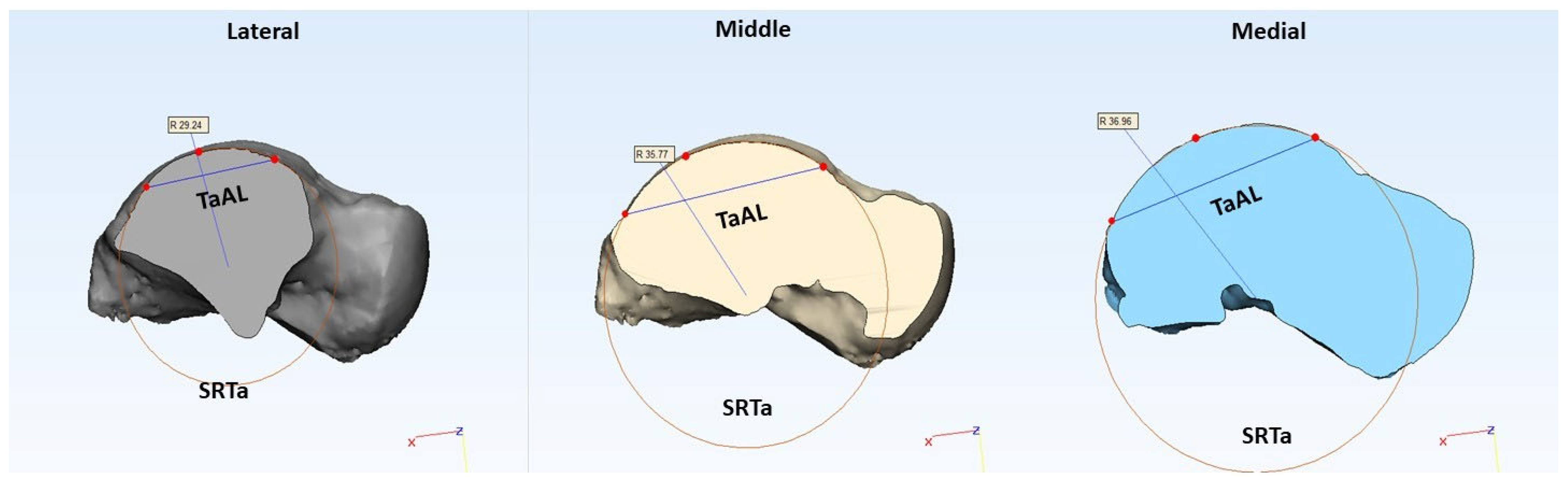
| TaAL (mm) | (medial, middle, lateral) | Trochlea tali arc length |
| SRTa (mm) | (medial, middle, lateral) | Trochlea tali radius |
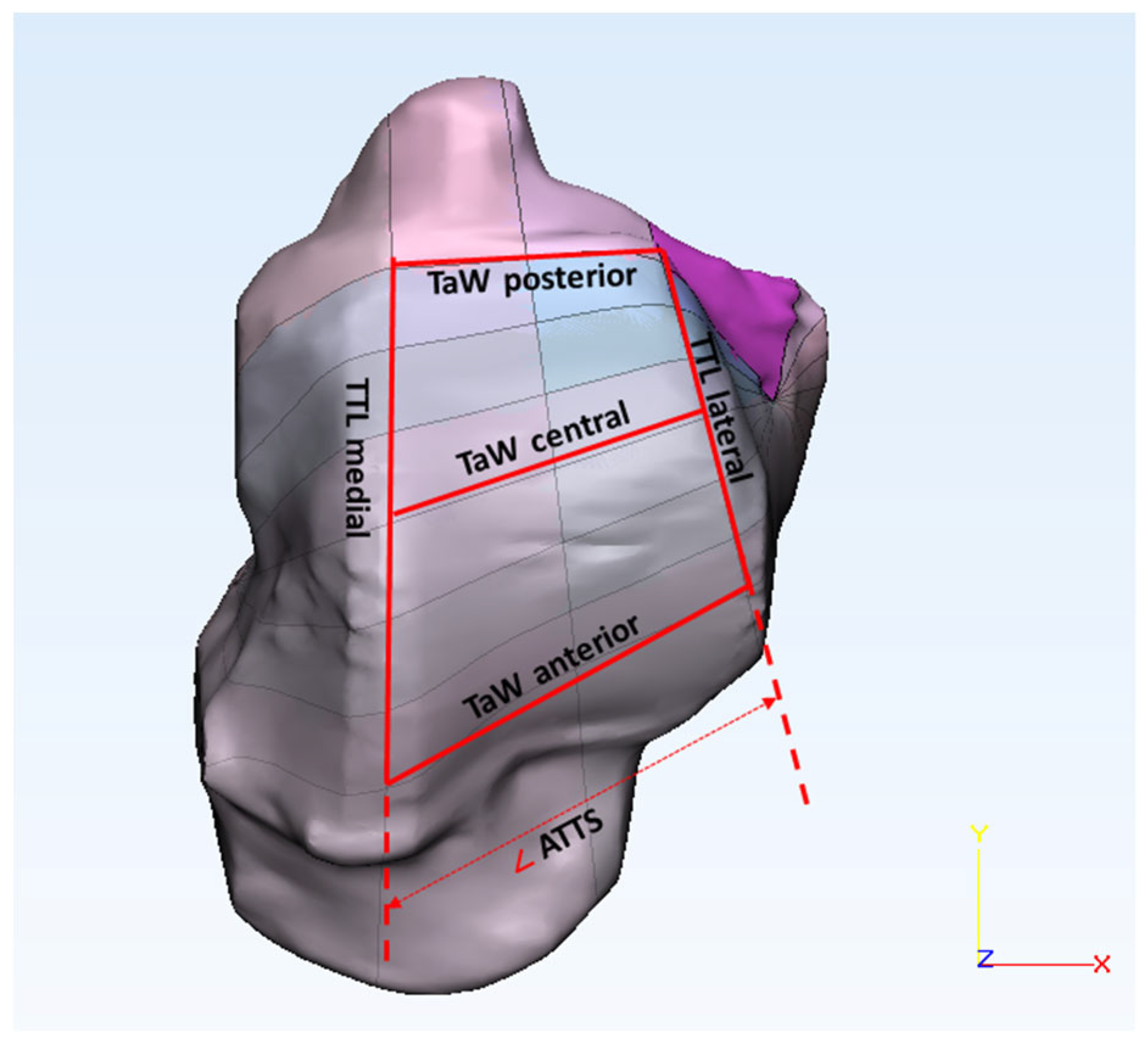
| TaW (mm) | (anterior, central, posterior) | Trochlea tali width |
| TTL (mm) | (medial, lateral) | Trochlea tali length |
| ATTS (deg) | - | Angle of trochlea tali shape |
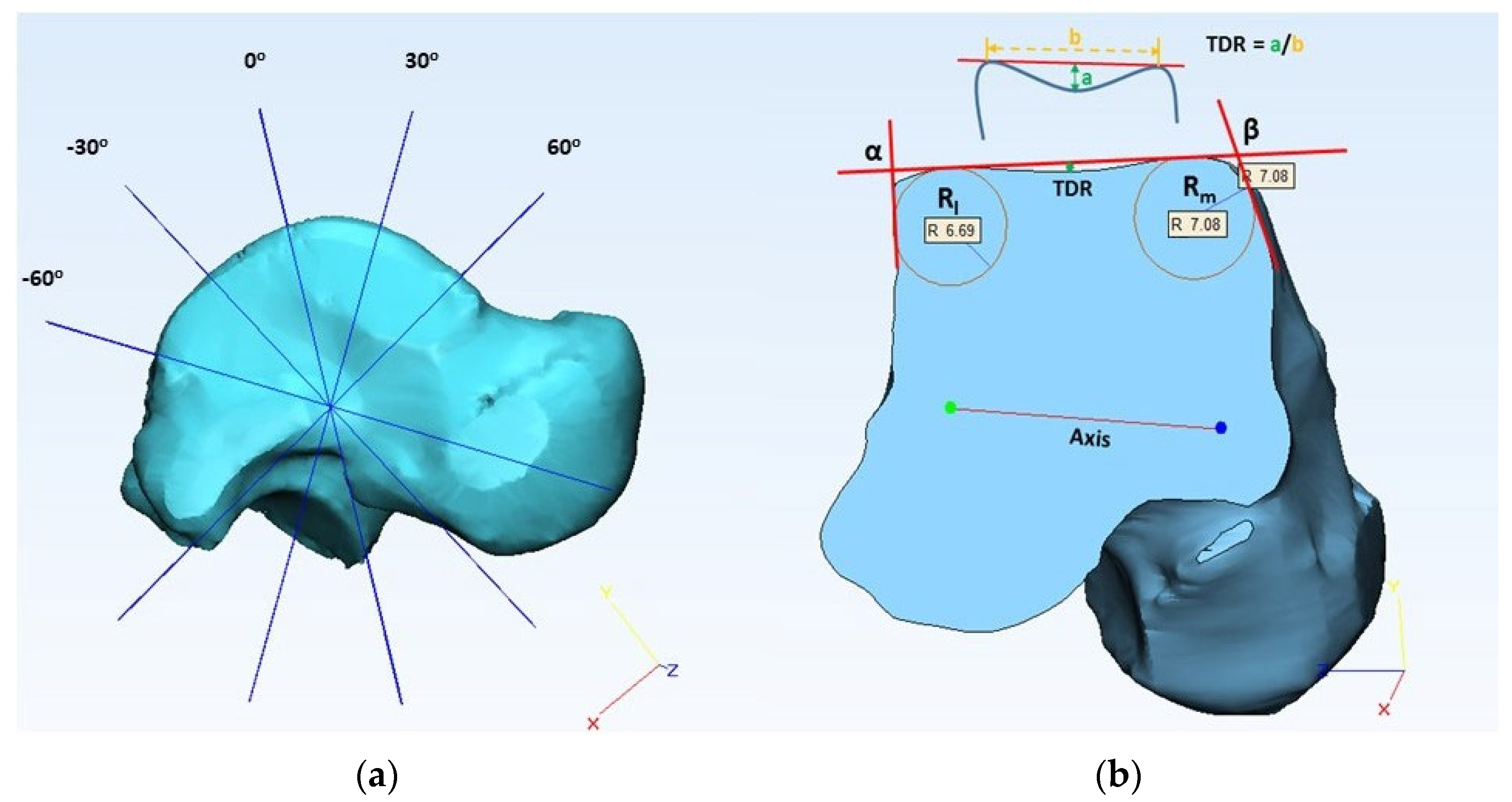
| TDR | (anterior, central, posterior) | Talus dome ratio |
| α (deg) | (anterior, central, posterior) | Lateral talar edge angle |
| β (deg) | (anterior, central, posterior) | Medial talar edge angle |
| Rl (mm) | (anterior, central, posterior) | Lateral frontal talar edge radius |
| Rm (mm) | (anterior, central, posterior) | Medial frontal talar edge radius |
| Talus Parameter | Tibia Parameter | Section | Equation | p-Value | R-Squared |
|---|---|---|---|---|---|
| SRTa | SRTi | Medial | SRTi = −1.987 + 1.213 × SRTa | <0.0001 | 0.723 |
| Middle | SRTi = 0.415 + 1.118 × SRTa | <0.0001 | 0.913 | ||
| Lateral | SRTi = 6.348 + 0.885 × SRTa | <0.0001 | 0.540 | ||
| TaW | TiW | Anterior | TiW = 2.259 + 0.925 × TaW | <0.0001 | 0.608 |
| Central | TiW = 3.907 + 0.9 × TaW | <0.0001 | 0.610 | ||
| Posterior | TiW = 6.175 + 0.822 × TaW | <0.0001 | 0.525 | ||
| TTL | TML | Medial | TML = −6.747 + 0.905 × TTL | <0.0001 | 0.848 |
| Lateral | TML = 11.433 + 0.411 × TTL | 0.0036 | 0.352 | ||
| ATMS | ATTS | - | ATMS = 5.337 + 0.731 × ATTS | 0.0269 | 0.222 |
Disclaimer/Publisher’s Note: The statements, opinions and data contained in all publications are solely those of the individual author(s) and contributor(s) and not of MDPI and/or the editor(s). MDPI and/or the editor(s) disclaim responsibility for any injury to people or property resulting from any ideas, methods, instructions or products referred to in the content. |
© 2023 by the authors. Licensee MDPI, Basel, Switzerland. This article is an open access article distributed under the terms and conditions of the Creative Commons Attribution (CC BY) license (https://creativecommons.org/licenses/by/4.0/).
Share and Cite
Gundapaneni, D.; Tsatalis, J.T.; Laughlin, R.T.; Goswami, T. Anthropomorphic Characterization of Ankle Joint. Bioengineering 2023, 10, 1212. https://doi.org/10.3390/bioengineering10101212
Gundapaneni D, Tsatalis JT, Laughlin RT, Goswami T. Anthropomorphic Characterization of Ankle Joint. Bioengineering. 2023; 10(10):1212. https://doi.org/10.3390/bioengineering10101212
Chicago/Turabian StyleGundapaneni, Dinesh, James T. Tsatalis, Richard T. Laughlin, and Tarun Goswami. 2023. "Anthropomorphic Characterization of Ankle Joint" Bioengineering 10, no. 10: 1212. https://doi.org/10.3390/bioengineering10101212
APA StyleGundapaneni, D., Tsatalis, J. T., Laughlin, R. T., & Goswami, T. (2023). Anthropomorphic Characterization of Ankle Joint. Bioengineering, 10(10), 1212. https://doi.org/10.3390/bioengineering10101212