Estimation of Low Flow Statistics for Sustainable Water Resources Management in South Australia

Abstract

The Magnitude and occurrence of extreme low flow events are needed in setting minimum flows to protect the instream users. As the true distribution is not normally known, the identification of the most appropriate distribution function that describes the extreme low flow data of a catchment is essential in estimating reliable low flow quantiles at various average recurrence intervals (ARI). The aim of this study is to conduct a comparative assessment of the performance of three plausible distribution functions for estimating low flow quantiles. The investigation was carried out by using 27-gauge stations within South Australia (SA), the driest state in Australia. The best distribution function out of the three selected distributions; Log Normal (LN), Log Pearson Type 3 (LP3), and Generalized Extreme Value (GEV for each of the three selected annual minima series (7-day, 15-day and 30-day) at each gauged catchments was identified. The estimated low flow quantiles from using these three distribution functions were compared using RMSE values estimated through Monte Carlo simulation studies. For the majority of the selected study catchments, GEV fitted using L moments was found to be the best method for estimating low flow quantiles at ARIs over 10 years (≥14%), while at low ARI, LP3 fitted using the Method of Moments (MOM) was shown to outperform (≥17%) the other methods.

1. Introduction

The effects of climate change are more evident and becoming a threat to the environmental system. This climate variability may significantly affect extreme weather changes, for instance, long term droughts or extreme floods [1]. Estimation of the reliable low flow regime of a stream is essential for water resources planning and management in water quality and quantity management studies, the planning of water supply schemes, flow diversions, hydropower generation, wildlife conservation, recreational uses, waste-load allocations into watercourses, reservoir storage design, and drought management. Many researchers emphasize that the characterization of the low flow statistics of a stream is important to improve the ability to predict the extreme low flow events for the water resource applications listed above [2,3,4]. Allocating environmental water flow from river systems is important for habitat protection, after fulfilling the basic demand of consumers [5]. As such, for some drainage basins, the flows need to be set to fulfil some specific predefined economic, ecological, or social objective. However, little attention has been directed towards low flow studies compared to flood studies [6]. Furthermore, there is ambiguity in recommended methods and, as a result, no standard procedure has been developed for estimating low stream flow statistics of catchments [2]. Therefore, identification of a suitable methodology for the data at hand and the assessment of low flow potential at various ARIs is needed for sustainable water resources management.

The availability of water resources in Australia is highly variable both in temporal and spatial means. This study is based on South Australia (SA), which is considered to be the driest state in Australia compared to the other states. Although a considerable amount of precipitation is received during the winter and early spring, which causes the streams to run, extreme climatic conditions (high evaporation) and catchment characteristics lead many streams to dry up entirely; thereby, resulting in streamflow patterns in SA that are highly variable and ephemeral. Furthermore, the permanent baseflow is reduced year by year depending on the preceding seasons’ rainfall. Therefore, the main water consumers, such as agriculture, mining, and energy related industries, need a good understanding of water availability and its variability for the efficient allocation of scarce water resources. Consequently, the development of methodologies to make accurate estimates of low flow regimes in South Australian streams is a fundamental need.

Although there have been some regional low flow studies conducted for South Eastern Australia [7,8,9], no such studies have been reported for SA. Hewa [10] conducted at-site low flow studies for Scott Creek and emphasized the importance of extending the same to the whole of SA. Therefore, the identification of a suitable methodology to quantify low flow potential of South Australian Rivers is a necessity.

There are studies that have investigated the applicability of different probability distribution functions for low flow frequency analyses [11,12,13,14,15,16]. For instance, the Gringorten plotting position formula and goodness-of-fit test have been applied to investigate the performance of different probability distribution methods for 25 British river catchments [12]. They recommended the use of P3 or GEV distributions for short durations while Generalized Pareto (GP) and GEV distribution for longer durations. Furthermore, they confirmed that the longer duration minima series does not follow the same distribution pattern as the short duration minima series. The Method of Moments (MOM) process is the oldest and the most widely understood technique for fitting frequency distributions [17]. Wallis et al. [16] documented the sample bias associated with skewness, whereas the authors of [17] documented the bias associated with both the skewness and the coefficient of variation of small and large samples drawn from highly skewed populations. However, the process of sampling the properties of bias and variance within these product moment estimators is distribution dependent [16].

The field of low flow frequency analysis has advanced substantially in recent times and a large number of techniques for representing the distribution function to a minima series have been introduced. For instance, fitting Generalized Extreme Value (GEV) distribution using LH moments [18] and LL moments [19]. The Expected Moment Estimate and Probability Plot Correlation are additional alternative methods for fitting a distribution function. The new techniques to fit the minima series are yet to be identified despite the above stated drawbacks of MOM, LN, and LP3, which are still fitted using MOM. Both Tasker [20] and Vogel and Kroll [21] recommended LP3/MOM, and according to Griffis et al. [22], USGS bulletin 17 proposes the use of the LP3 with a conditional probability adjustment. The ease of computing the parameters and conceptual simplicity are the primary advantages of the MOM estimators technique [17]. Furthermore, low flow frequency analyses for Scott Creek catchment in SA showed that all four models LN/MOM, LP3/MOM, GEV/L, and GEV/L2 performed equally at low to medium ARIs, while GEV/L2 values were more conservative when compared with those from the other models [10]. Accordingly, this study extends the work performed by the authors of [10] to the remaining SA catchments for the purpose of identifying a model which performs better for the majority of the catchments in the region.

The aim of this study is to identify the most suitable distribution function for estimating low flow quantiles at six selected ARIs for extreme low flow series of three durations (7-day, 15-day, and 30-day) at 27 selected South Australian catchments. The best distribution function for SA catchments was identified from four plausible models: LN/MOM, LP3/MOM, GEV/L, and GEV/L2. Suitability of these models for describing the selected annual minima series of the selected study catchments was assessed by using probability plots, while the reliability of the estimated low flow quantiles was assessed using RMSE values estimated through Monte Carlo simulation studies.

2. Materials and Methods

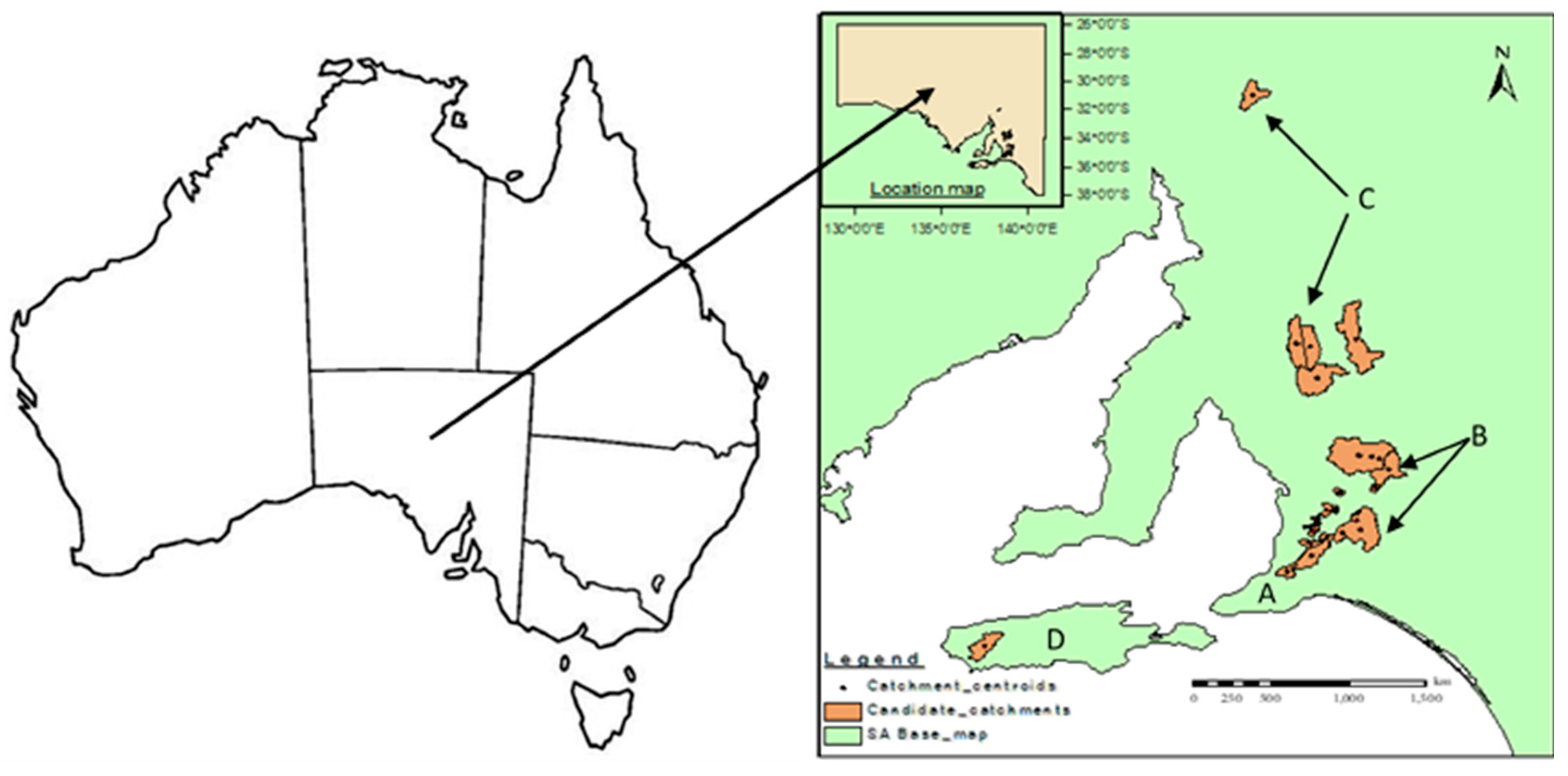
2.1. Study Area

The study catchments were selected from four regions of South Australia, namely, Adelaide and Mt Lofty, Northern and York, SA Murray–Darling Basin, and Kangaroo Island. The geographical distributions of the candidate catchments of the study area are shown in Figure 1.

Table 1. Details of the study catchments.

Station No	Station Name	Record Length (Years)	Catchment Area (km2)	Major River Basin	Region	Region Reference
4260504	4 KM East of Yundi	37	191.0	Lower Murray river	SA Murray–Darling Basin	A
4260529	U/S Cambrai	15	239.0
4260533	Near Hartley	14	473.0
4260536	Worlds end	30	704.0
4260557	D/S Mt. Barker	18	88.0
4260558	Dawesley	28	43.0
5020502	U/S Dam and Rd Br	10	76.5	Myponga	Adelaide and Mt. Lofty	B
5030502	Scott Bottom	37	26.8	Onkaparinga
5030503	4.5 KM Wnw Kangarilla	18	48.7
5030506	U/S Mt Bold Res.	17	34.2
5030507	Lenswood	15	16.5
5030508	Craig bank	30	8.4
5030509	Aldgate Rly Station	15	7.8
5030526	Uraidla	11	4.3
5040512	Mt Pleasant	33	26.0	Torrens River
5040517	Waterfall Gully	13	5.0
5040518	U/S Minno Ck Junction	13	19.0
5040523	Castambul	15	44.0
5040525	U/S Millbrook Res	12	23.0
5050502	Yaldara	18	384.0	Gawler River
5050504	Turretfield	34	708.0
5050517	Penrice	16	118.0
5060500	Near Rhynie	27	417.0	Wakefield River	Northern and York	C
5070500	Near Andrews	29	235.0	Broughten River
5070501	Near Spalding	31	280.0
5090503	Old Kanyaka Ruins	21	180.0	Willochra Creek
5130501	U/S Gorge Falls (K.I.)	33	190.0	Kangaroo Island	Kangaroo Island	D

provides basic information about the selected gauge stations/catchments. The selection of these catchments was primarily based on the degree of urbanization assessed using data from land use surveys published by Data SA in 2008, 2014, and 2016, in addition to, the amount of regulation, the length, and the quality of the observed stream flow data series. Small to medium unregulated catchments (A < 1000 km²) with less than 10% urbanization and over ten years of high-quality daily flow data were selected for the investigation.

The selected catchments cover a diverse climatic and physiographic conditions. Mean annual rainfall over the study area varies from 300 mm to 1000 mm while mean annual class A pan evaporation varies from 1200 mm to 3200 mm (Bureau of Meteorology, 2010). Elevation of the selected catchments varies from 0 m AHD to 450 m AHD.

2.2. Data Collection

Daily stream flow data recorded based on the calendar year of the selected catchments were obtained from the Department for Environment and Water in SA. Available stream flow data for the majority of the catchments were impaired by various quality issues including missing records and unknown or not collected data. Therefore, the stream flow data of each catchment was subjected to an initial screening to remove all doubtful information. Consequently, 27 catchments with good quality streamflow data were retained for the initial study (Table 1). For this investigation, three annual minima series were extracted: 7-day, 15-day, and 30-day.

2.3. Fitting Distribution Functions to the Observed Minima Series

As stated in Section 1, the aim of this study is to investigate the performance of four models: LN/MOM, LP3/MOM, GEV/L, and GEV/L2, in analyzing three annual minima series of the 27 selected catchments in SA (Table 1). However, due to the lack of sufficient nonzero annual minima in the extracted series, only 15 catchments were considered in the final investigation. At the start, probability plots of the minima series were ranked in ascending order and constructed using Cunnane’s plotting position formula. Subsequently, low flow quantiles at six selected recurrence intervals were estimated and plotted on the probability plot in order to view how best each model type describes the observed minima series of the study catchment. In order to understand the reliability of the model estimates, the RMSE of each flow quantile was estimated using the Monte Carlo simulation process (Figure 2). As the actual distribution of where data has come from is usually unknown, the Monte Carlo simulation was repeated by taking each model type as the parent distribution at a given time and estimating low flow quantiles using the remaining model types as well as estimating the RMSE (Equation (1)) of the low flow quantiles at each selected ARI.

$$RMSE=\sqrt{{{\displaystyle \sum }}_1^N{\left(Q_i-\overline{Q}\right)}^2}$$

(1)

where;

• $Q_i$= Low flow quantile
• $\overline{Q}$ = Mean quantile
• $N$ = Random sample number
• $RMSE$ = Root mean square error

The specific details of this two-stage investigation process are discussed next.

For each of the selected study catchments, low flow quantiles at six ARIs (ARI = 2, 5, 10, 20, 50, 100) were estimated for the three selected annual minima series (7-day, 15-day, and 30-day) using LN, LP3, and GEV distributions. The LN and LP3 were fitted by using MOM with conditional probability adjustment, which is a methodology that has been well documented in many studies [10,23]. GEV distribution function was fitted to the annual minima series by using both L moments and L2 moments; the methodology is well documented in Hewa et al. [18]. Consequently, a total of four model types: LN/MOM, LP3/MOM, GEV/L, and GEV/L2 were fitted to the data series. In the second stage, Monte Carlo simulations were performed as discussed next.

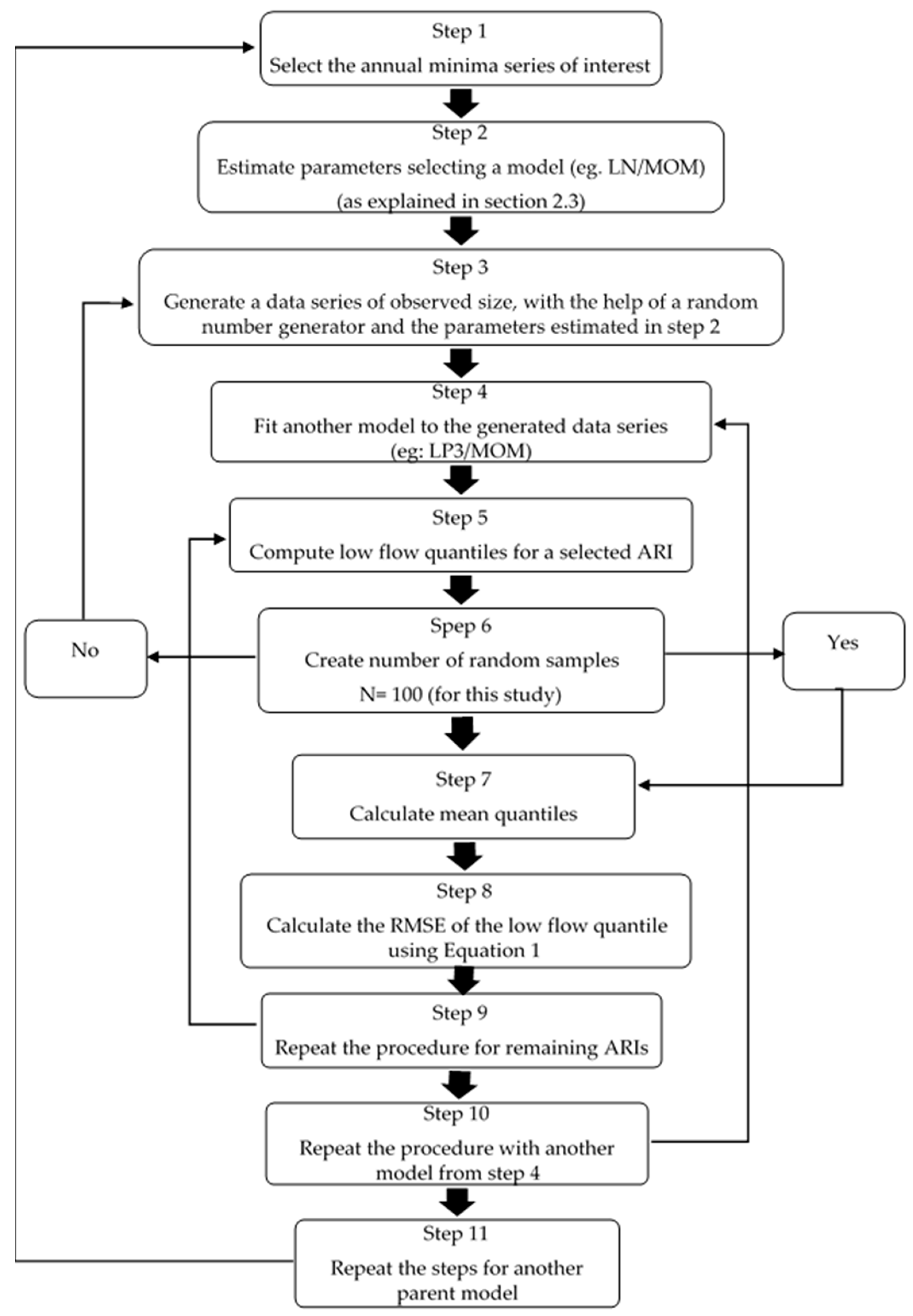
2.4. Monte Carlo Simulations

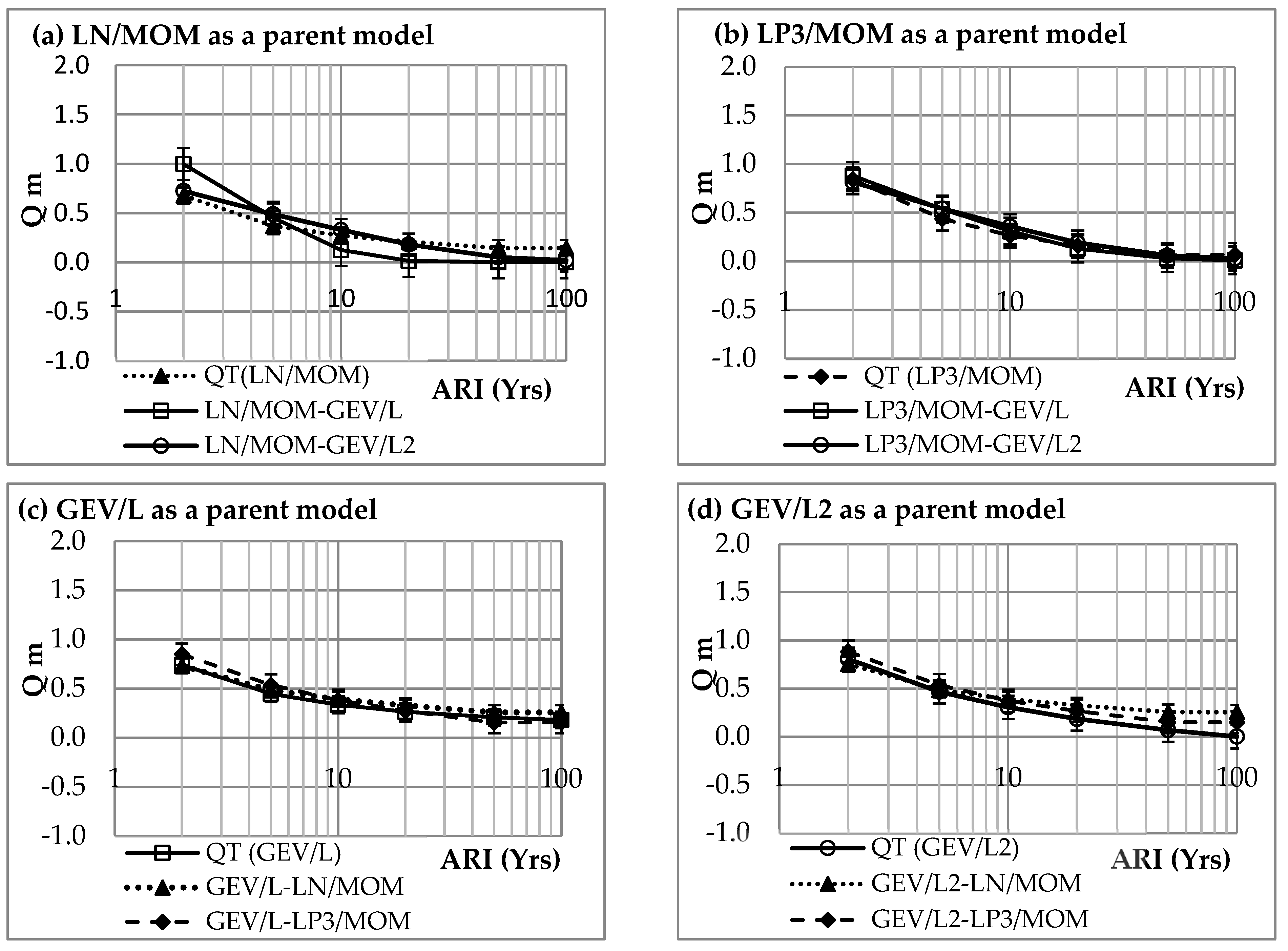
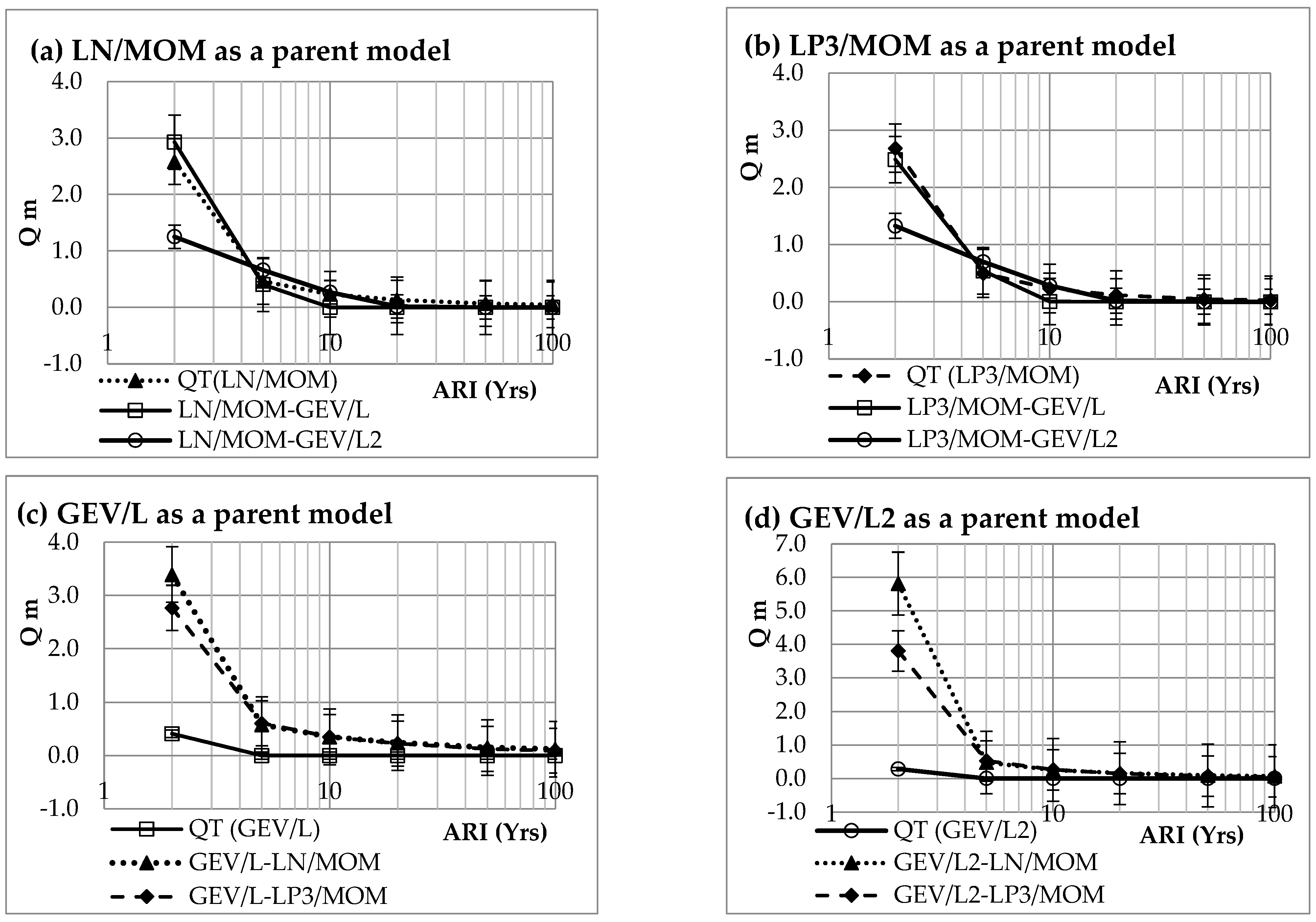
Monte Carlo simulations were carried out to investigate how each model performs when the data are derived from another model. The Monte Carlo method is the practical alternative framework proposed by the International Organization for Standardization (ISO) guide 98–3 for the evaluation of uncertainty in measurement [24]. As discussed by Hewa [10], when presented with a selected parent model (e.g., LN/MOM), a Monte Carlo Simulation was conducted as described in the flow chart (Figure 2).

3. Results

The 7-day 10-year low flow quantile (Q _7,10) is one of the most widely used low flow indexes worldwide; therefore, the results are mainly demonstrated by using this low flow index. Of the 27 selected catchments, one (A5040525) had no nonzero flows and was subsequently excluded from the analyses. Three other catchments (A4260533, A5030508, and A5040512) had only 1 or 2 nonzero observations and were not able to fit any of the models; they were thus excluded from the analyses. Furthermore, of the 23 remaining catchments, GEV (L or L2) fitting failed at another 8 catchments due to insufficient nonzero flow observations. Therefore, model performance is compared using only 15 catchments to which all four models can be fitted.

Table 2. Estimated Q _{7, 10} by the four models.

Station No	LN/MOM (Ml)	LP3/MOM (Ml)	GEV/L (Ml)	GEV/L2 (Ml)
A4260504	0.36	0.35	0.00	0.00
A4260536	6.96	6.70	7.32	6.59
A4260557	0.23	0.23	0.00	0.00
A5020502	0.11	0.11	0.00	0.00
A5030502	0.25	0.25	0.07	0.06
A5030503	0.28	0.28	0.02	0.00
A5030506	0.39	0.39	0.40	0.39
A5030509	0.13	0.13	0.00	0.03
A5030526	0.27	0.27	0.33	0.30
A5040517	1.61	1.59	1.58	1.54
A5040518	0.73	0.74	0.64	0.65
A5040523	3.23	3.70	1.41	2.07
A5050517	0.34	0.36	0.06	0.00
A5060500	4.03	4.36	2.45	4.08
A5070500	2.48	2.40	0.01	0.01

provides the quantile estimates made by each of the four models for these catchments.

It is observed from Table 2 that GEV/L and GEV/L2 estimates of 7-day 10-year low flow quantiles are greatly different to those of LN/MOM and LP3/MOM models for a majority of the catchments except for A4260536, A5030506, A5030526, A5040517, A5040518, and A5060500. These six catchments are wet or fairly wet catchments. For all the other catchments, LN/MOM and LP3/MOM means are higher compared to GEV/L and GEV/L2 models. A5070500 is the driest catchment out of all other dry catchments—having 83% of zero observations. This catchment is located in the Northern and York region, which has had more hot days over 38 °C in the past 30 years (1989–2018) [25].

Figure 3 compares the 7-day mean quantile of a wet catchment when the data is generated from another model. It is clearly observed from Figure 3b,c that, when the data is derived from LP3/MOM or GEV/L, other models make equally close estimates at every ARI considered. However, when LN/MOM is considered as the parent, both GEV/L and GEV/L2 models overestimate the risk (i.e., underestimate the low flow quantile). On the other hand, when GEV/L2 is considered as the parent, every other model makes underestimations of the risk (i.e., overestimates the low flow quantile) and, importantly, the deviation from the parent is greater at higher ARIs for wet catchments.

In contrast, Figure 4 compares the 7-day mean quantile of a dry catchment when the data is generated from another model. It is observed from Figure 4a,b,d that when data are generated by taking LN/MOM, LP3/MOM, or GEV/L2 as parent models, other models perform equally or in a similar pattern for high ARIs. However, when GEV/L or GEV/L2 are considered as the parent model, every other model underestimates the risk (i.e., overestimates the low flow quantile) and the deviation from the parent is greater at lower ARIs. This means, if the data are coming from GEV, then other models underperform. On the other hand, even when data come from other distributions, GEV/L performs well.

Figure 5 compares the models using RMSE of the 7-day low flow quantiles estimates at six selected ARIs for the 15 catchments. The model with the least RMSE was given rank one while equal rank was given when RMSE of two models are the same. At higher ARIs, estimation of RMSE was not possible as the quantile estimates become zero; consequently, no ranking was performed at those quantiles (e.g., GEV/L2 → LN/MOM at ARI over 10 years). The maximum height that a column in Figure 5 can reach is up to 100%. It is noted that, when data is derived from either LN/MOM or LP3/MOM, both GEV/L and GEV/L2 are suitable to make quantile estimates at higher ARIs. However, no model consistently performs better for the region at low ARIs. The low quality data and zero flows may have contributed to inconsistent analysis.

Figure 6 presents the overall results when the performance of the four models over all three selected series is considered. It compares how each model performs when a data series is drawn from the other models. The Y axis of Figure 6 indicates the percentage of occurrences that each model made for the quantiles with the least RMSE. It is observed from Figure 6 that GEV/L was consistently the best performer with ARIs over 10 years while LP3/MOM outperforms with low ARIs.

4. Discussion

There are different definitions for low flow in the literature. Many studies describe it as the actual streamflow during the dry period while others consider the changes to streamflow between consecutive flood events [26]. The study of low streamflow and return periods associated with extreme events is highly significant for effective water supply and sustainable management of water in a given region or country. The low flow condition is mainly linked with climatic conditions and catchment characteristics. It may vary daily, seasonally, and annually. Accordingly, there are different measures and indices used to characterize the low flow, for instance: mean daily flow, median flow, mean annual runoff, and absolute minimum flow [27]. As the low flow condition is linked with climatic and geophysical conditions, a model developed for one region may not perform equally for estimating the low streamflow statistics of another region. Therefore, choosing the best fitting frequency distribution model to evaluate the extreme low flow events in a region is a common problem in hydrology. Accordingly, this study was conducted using four models—namely, LN/MOM, LP3/MOM, GEV/L, and GEV/L2—to estimate the low flow quantiles of SA catchments.

We noticed that when the catchments are wet or fairly wet, any of the four models (LN/MOM, LP3/MOM, GEV/L, and GEV/L2) make fairly equal quantile estimates. For dry catchments, LN/MOM and LP3/MOM models overestimate when compared to GEV/L and GEV/L2 models. As low flows are more important in dry catchments than wet catchments, it is very important to know which model makes the most accurate estimates of low flow quantiles in dry catchments. The results were further investigated using 7-day mean quantiles of six selected ARIs: 2, 5, 10, 20, 50, and 100, when data are generated from another model as in Figure 3 and Figure 4. It is clearly evident that there is no single model that consistently performs better. The models perform differently for wet and dry catchments. This may be due to unavoidable data quality issues in the obtained data, for instance, missing stream flow observations for a varying length, short record length, limited number of gauge catchments, and unrealistically high recorded values. It could even be due to the fact that high frequency and low frequency flows have different trends. Of the initial 27 catchments, twelve catchments had no or insufficient nonzero flow observations to fit with one or more distribution functions; therefore, they were excluded from the study. The analysis continued with only 15 catchments.

The performance of each model was further compared using the RMSE value of the 7-day low flow quantiles. Figure 5 shows that GEV/L and GEV/L2 are the most suitable models for evaluating the low flow quantiles of higher ARIs while Figure 6 confirmed the use of GEV/L model for medium to high ARIs. Moreover, LP3/MOM can be a good candidate for estimating low flow quantiles at low ARIs. However, the results of this study emphasize the significant importance of developing new techniques for estimating low flow quantiles of catchments given several data restrictions. Ouarda et al. [28] outlined that flood frequency analysis methods, such as neighbourhood regionalization approach, can be extended to estimate low-flow quantiles. In a recent study [29], the canonical correlation and neural network based regional frequency analysis method were used to estimate low flow in South Korean river basins. Jung et al. [29] highlighted that the machine learning-based nonlinear model could estimate relatively reliable low-flow quantiles compared to a linear model. The most commonly used methods in low flow analysis are: Weibull, Gumbel, Log–Normal, Gamma, Pearson Type III, and Log–Pearson Type III [2,28]. This study confirmed that the Method of Moment (which is used in this study) or other methods, such as the probability weighted moment method, could be used for estimating parameters of the selected distribution functions. Furthermore, due to the absence of stream flow data or the short length of records, there is a high level of uncertainty in selecting the best fit distribution function for estimating low flow quantiles. In such cases regional frequency analysis is the most commonly used method for estimating extreme events (flood or droughts)—where no or little flow data is available [28,30].

Furthermore, there is an increasing demand for a reliable estimate of low flow quantiles for many economic and environmental applications. As such, improving the existing developed methods or developing efficient techniques for the accurate estimation of low flow quantiles is important.

5. Conclusions

South Australia is considered the driest state in Australia, and its streamflow patterns are highly variable and ephemeral. Moreover, permanent baseflow reduces year by year depending on the preceding seasons’ rainfall. Climate variability greatly affects the frequency and severity of extreme flow events; thereby stressing the importance of increasing the frequency of hydrological drought alarms; developing best fit models for the projection of extreme low flow events; mitigating uncertainty in function selection; and synthesizing existing knowledge [31,32]. Consequently, the development of methodologies to estimate low flow regimes in SA streams is fundamental to efficient water allocation.

Low flow frequency analyses of three annual minima series from SA catchments were conducted using four models: LN/MOM, LP3/MOM, GEV/L, and GEV/L2. The performance of each model was compared against the other by using RMSE values. Monte Carlo simulations were conducted to compute the RMSE of the quantile estimates made from each model when the data series were derived from another model. It was noted that no single model consistently outperforms the others for the entire range of the selected ARIs in SA catchments. The results support the use of GEV/L for estimating low flow quantiles at medium to high ARIs, while LP3/MOM outperforms at low ARIs.

Poor quality records, unavailability of long-term stream flow records, and having a limited number of gauge catchments have restricted the comparative analyses to 15 catchments. Therefore, in order to obtain a reliable relationship between catchment characteristics and low flow index further research should be carried out. As the second stage of the study, the authors are planning to develop a regional regression model for ungauged catchment predictions in SA. The success of the regional regression model for low flow regimes depends on the data availability. An absence of high-quality records or missing data will greatly affect the final outcome. The identified data quality issues in the study area are: unrealistically high values, short record length, and varying lengths of missing data for a period of one day to several years. Therefore, the compilation of a good, quality database for SA is necessary if reliable low flow predictions are to be made. Increasing the length of available gauge flow data by filling the gaps/missing data would be an alternative measure that could be taken to improve the reliability of the estimates of low flow quantiles.

Moreover, this study emphasizes the importance of developing alternate methodologies or techniques for quantifying the low flow regimes of catchments with short records or no flow records.

References

1. Thornton, P.K.; Ericksen, P.J.; Herrero, M.; Challinor, A.J. Climate Variability and Vulnerability to Climate Change: A Review. Glob. Chang. Biol. 2014, 20, 3313–3328. [Google Scholar] [CrossRef] [PubMed]
2. Kroll, C.N.; Vogel, R.M. Probability Distribution of Low Streamflow Series in the United States. J. Hydrol. Eng. 2002, 7, 137–146. [Google Scholar] [CrossRef] [Green Version]
3. Yue, S.; Pilon, P. Probability Distribution Type of Canadian Annual Minimum Streamflow. Hydrol. Sci. J. 2005, 50, 427–438. [Google Scholar] [CrossRef]
4. Yue, S.; Wang, C.Y. Possible Regional Probability Distribution Type of Canadian Annual Streamflow by L-Moments. Water Resour. Manag. 2004, 18, 425–438. [Google Scholar] [CrossRef]
5. Acreman, M.; Dunbar, M. Defining Environmental River Flow Requirements—A Review. Hydrol. Earth Syst. Sci. 2004, 8, 861–876. [Google Scholar] [CrossRef]
6. Kroll, C.; Luz, J.; Allen, B.; Vogel, R.M. Developing a Watershed Characteristics Database to Improve Low Streamflow Prediction. J. Hydrol. Eng. 2004, 9, 116–125. [Google Scholar] [CrossRef] [Green Version]
7. Nathan, R.J.; McMahon, T.A. Overview of a Systems Approach to the Prediction of Low Flow Characteristics in Ungauged Catchments. In National Conference Publication; Institution of Engineers, Australia: Barton, Australia, 1991; Volume 1, pp. 187–192. [Google Scholar]
8. Nathan, R.J.; McMahon, T.A. Estimating Low Flow Characteristics in Ungauged Catchments. Water Resour. Manag. 1992, 6, 85–100. [Google Scholar] [CrossRef]
9. Hewa, G.H. A Methodology for Regional Low Flow Frequency Analysis. Doctoral Dissertation, University of Melbourne, Melbourne, Australia, 2001. [Google Scholar]
10. Hewa, G.A. Comparing the Performance of Four Selected Models in Low Flow Frequency Analyses—A Case of Scott Creek in South Australia. In 31st Hydrology and water resources symposium and the 4th International Conference on Water Resources and Environment Research 2008; Engineers Australia: Barton, Australia, 2008. [Google Scholar]
11. Zaidman, M.D.; Keller, V.; Young, A.R. Low Flow Frequency Analysis Guidelines for Best Practice; Environment Agency: Bristol, UK, 2002. Available online: https://assets.publishing.service.gov.uk/government/uploads/system/uploads/att (accessed on 6 August 2022).
12. Zaidman, M.D.; Keller, V.; Young, A.R.; Cadman, D. Flow-Duration-Frequency Behaviour of British Rivers Based on Annual Minima Data. J. Hydrol. 2003, 277, 195–213. [Google Scholar] [CrossRef]
13. Escalante-Sandoval, C.A. Mixed Distributions in Low-Flow Frequency Analysis. Ing. Investig. Tecnol. 2009, 10, 247–253. [Google Scholar] [CrossRef]
14. Patel, J.A. Evaluation of Low Flow Estimation Techniques for Ungauged Catchments. Water Environ. J. 2007, 21, 41–46. [Google Scholar] [CrossRef]
15. Vivekanandan, N.; Poornima, R. A Study on Comparison of Probability Distributions for Frequency Analysis of Low-Flow. Civ. Eng. Res. J. 2021, 11, 72–78. [Google Scholar] [CrossRef]
16. Wallis, J.R.; Matalas, N.C.; Slack, J.R. Just a Moment! Water Resour. Res. 1974, 10, 211–219. [Google Scholar] [CrossRef] [Green Version]
17. Vogel, R.M.; Fennessey, N.M. L-Moments Diagram Should Replace Product Moment Diagrams. Water Resour. Res. 1993, 29, 1745–1752. [Google Scholar] [CrossRef]
18. Hewa, G.A.; Wang, Q.J.; McMahon, T.A.; Nathan, R.J.; Peel, M.C. Generalized Extreme Value Distribution Fitted by LH Moments for Low-Flow Frequency Analysis. Water Resour. Res. 2007, 43, W06301. [Google Scholar] [CrossRef] [Green Version]
19. Durrans, S.R.; Tomic, S. Comparison of Parametric Tail Estimators for Lowflow Frequency Analysis. J. Am. Water Resour. Assoc. 2001, 37, 1203–1214. [Google Scholar] [CrossRef]
20. Tasker, G.D. Regionalization of Low Flow Characteristics Using Logistic and GLS Regression. In New Directions for Surface Water Modeling (Proceedings of the Baltimore Symposium); Kavvas, M.L., Ed.; International Association of Hydrological Sciences Publication (IAHS) Publication: Baltimore, MD, USA, 1989; pp. 323–331. [Google Scholar]
21. Vogel, R.M.; Kroll, C.N. Low-Flow Frequency Analysis Using Probability-Plot Correlation Coefficients. J. Water Resour. Plan. Manag. 1989, 115, 338–357. [Google Scholar] [CrossRef] [Green Version]
22. Griffis, V.W.; Stedinger, J.R.; Cohn, T.A. Log Pearson Type 3 Quantile Estimators with Regional Skew Information and Low Outlier Adjustments. Water Resour. Res. 2004, 40, W07503. [Google Scholar] [CrossRef]
23. Tallaksen, L.; Hewa, G. Extreme Value Analysis. In Manual on Low-Flow Estimation and Prediction; World Meteorological Organization: Geneva, Switzerland, 2008. [Google Scholar]
24. International Organization for Standardization (ISO). ISO IEC Guide 98-3—Uncertainty of Measurement—Part 3: Guide to the Expression of Uncertainty in Measurement (GUM;1995); ISO: Geneva, Switzerland, 2008; Available online: https://www.iso.org/standard/50461.html (accessed on 6 August 2022).
25. Bureau of Meteorology and the CSIRO. Regional Weather and Climate Guide. Available online: http://www.bom.gov.au/climate/climate-guides/guides/050-Northern-and-Yorke-SA-Climate-Guide.pdf. (accessed on 6 August 2022).
26. Smakhtin, V.U. Low Flow Hydrology: A Review. J. Hydrol. 2001, 240, 147–186. [Google Scholar] [CrossRef]
27. Lee, K.S.; Kim, S.U. Identification of Uncertainty in Low Flow Frequency Analysis Using Bayesian MCMC Method. Hydrol. Process. 2008, 22, 1949–1964. [Google Scholar] [CrossRef]
28. Ouarda, T.B.M.J.; Charron, C.; St-Hilaire, A. Statistical Models and the Estimation of Low Flows. Can. Water Resour. J. 2008, 33, 195–206. [Google Scholar] [CrossRef] [Green Version]
29. Jung, K.; Kim, E.; Kang, B. Estimation of Low-Flow in South Korean River Basins Using a Canonical Correlation Analysis and Neural Network (CCA-NN) Based Regional Frequency Analysis. Atmosphere 2019, 10, 695. [Google Scholar] [CrossRef] [Green Version]
30. Khan, M.S.U.R.; Hussain, Z.; Ahmad, I.; Noor, F. Modeling of Flood Extremes Using Regional Frequency Analysis of Sites of Khyber Pakhtunkhwa, Pakistan. J. Flood Risk Manag. 2021, 14, e12751. [Google Scholar] [CrossRef]
31. Wilhite, D.; Svoboda, M. Drought Early Warning Systems in the Context of Drought Preparedness and Mitigation, in Early Warning Systems for Drought Preparedness and Drought Management; National Drought Mitigation Center: Lincoln, NE, USA, 2000. [Google Scholar]
32. Sheffield, J.; Wood, E. Projected Changes in Drought Occurrence under Future Global Warming from Multi-Model, Multi-Scenario, IPCC AR4 Simulations. Clim. Dyn. 2007, 31, 79–105. [Google Scholar] [CrossRef]
Figure 1. Geographical locations of the drainage basins considered in the current study.
Hydrology 09 00152 g001
Figure 2. Simulation process.
Hydrology 09 00152 g002
Figure 3. Comparison of the 7-day mean quantile estimate (Qm) of catchment A5030526 (wet catchment) at Uraidla when data generated from another model. Error bars indicate standard error.
Hydrology 09 00152 g003
Figure 4. Comparison of the 7-day mean quantile estimate (Qm) of catchment A4260557 (dry catchment) at D/S Mt. Barker when data were generated from another model. Error bars indicate standard error.
Hydrology 09 00152 g004
Figure 5. Comparison of the models using RMSE of 7-day minima series of the study catchments.
Hydrology 09 00152 g005
Figure 6. Comparison of the performance of four selected models in analyzing three selected series (7-day, 15-day, and 30-day).
Hydrology 09 00152 g006