1. Introduction
Performing accurate flood forecasts in terms of the location, magnitude, and timing of runoff and flooding remains a key challenge, especially for intense convective rainfall events affecting Mediterranean areas. This need is particularly acute given the potential intensification of the frequency of extreme precipitation in this region (e.g., [
1,
2,
3]), in which the Mediterranean climate is characterized by a significant variability, with warm and dry summers and heavy rainfall events in autumn [
4]. Nevertheless, given the complexity of the hydro-meteorological processes involved and their heterogeneous and limited observability, flash flood hydrological modeling remains a hard task, and internal fluxes are generally tinged with large uncertainties. It is therefore important to study how and why hydrological models of different complexities perform in simulating flash flood hydrological response.
The “resolution–complexity continuum” [
5] has been investigated over the past five decades by many studies with various modeling approaches, ranging from point-scale processes numerically integrated at larger scales (e.g., catchment) to spatially lumped representation of the system response [
6]. Among the variety of existing hydrological models, and the hypotheses they rely on, their components generally describe water storage and transfer (e.g., [
7]) via various combinations and parameterizations of vertical and lateral storage-flux operators.
We mention that all hydrological models are, to some degree, conceptual, and due to limitations and uncertainties in their structure, parameters’ representativity, data availability, and even, initial and boundary conditions, calibration/learning is generally required. Besides, whatever their status and complexity, hydrological models are most often calibrated and validated using observed discharge time series at the outlet of a catchment [
8], i.e., integrative data containing the mixed signature of all upstream processes. However, multiple model configurations and associated parameters can lead to a similar value of discharge (equifinality problem [
9,
10]). Whereas a model can be capable of reproducing the system response (e.g., discharge) it has been trained for, it can fail in reproducing meaningful system internal dynamics and patterns [
6], thus providing the right answers for the wrong reasons [
11]. Then arises the problem of better calibrating/validating hydrological models, and in particular distributed models, which makes it possible to take into account the spatial variabilities in the properties of the basins and atmospheric signals, to simulate spatialized hydrological quantities, but confronted with the problem of over-parameterization and equifinality (see the discussion in Grayson and Blöschl [
12] and Jay-Allemand et al. [
13] in a flash flood context with the spatially distributed calibration of the SMASH model). For physical models, Grayson and Blöschl [
12] commented that “mimicking real processes adds complexity, which in turn expands the amount and type of data needed”.
A key factor for flash flood simulation, in addition to river discharge, is surface runoff controlled by soil infiltration rates [
14,
15,
16]. Reaching a coherent representation of state fluxes’ variabilities both at the outlet and within catchments remains a challenge in spatially distributed modeling, which could be moved ahead using the information from hydrological signatures (see the review in [
17] and the references in [
18]) in combination with sensitivity analysis [
19]. Information selection and a distributed model constraint can benefit from sensitivity analysis, as done with the MARINE model for flash flood Mediterranean catchments by [
20] or [
21], guiding the design of regionalization methods accounting for bedrock types, among other descriptors [
22]. In the case of Mediterranean flash floods, Eeckman et al. [
23] recently assessed multi-hypothesis modeling of subsurface flows [
15] with MARINE using multi-source local and gridded soil saturation signatures. Flash flood models’ comparisons and analysis are still needed, especially in terms of performances in reproducing multi-scale signatures associated with state fluxes.
Previous studies, aiming at analyzing the differences between modeling approaches of various complexities, through several model comparison experiments, tested the performances in terms of stream flow modeling (see [
24,
25,
26,
27]), but also in terms of the internal state, such as soil moisture (cf. [
18,
28,
29] and the references therein). However, few cases have focused on flash floods. Koch et al. [
28] compared three distributed hydrological models of different complexities in the way they simulated seasonal soil moisture patterns of a small forested catchment. They concluded that including parameters related to soil properties and topography improved the performance of the models in terms of the soil moisture. Orth et al. [
29] concluded that “added complexity does not necessarily lead to improved performance of hydrological models, and that performance can vary greatly depending on the considered hydrological variable (e.g., runoff vs. soil moisture) or hydrological conditions (floods vs. droughts).” Ludwig et al. [
30] investigated the effect of model complexity on the impact assessment of climate change and concluded that the degree of complexity does have an impact on the predictive performance and that process representation is invaluable.
Other studies include that of Lobligeois et al. [
31] on several catchments in France to check the effect of higher-resolution rainfall and conceptual model resolution on stream flow simulation. They showed that a semi-distributed approach based on the GR4 model [
32] performed better than the lumped one for the Cévennes and Mediterranean regions, where the rainfall spatial variability is very high. Grayson and Blöschl [
12] showed that the spatio-temporal variability of soil moisture was reproduced by a distributed model accounting for the effect of spatial variability in topography on lateral surface and subsurface flow, among others. Boithias et al. [
33] compared the performance of the distributed event-based MARINE model and the lumped continuous SWAT model in flash flood modeling for a French Mediterranean catchment and found that, while the MARINE model simulated the peak and timing better, the SWAT model was better at simulating the recession discharge and the exported water volume. Jay-Allemand [
34] proposed a variational (assimilation) algorithm and showed its potential for the spatially distributed calibration of SMASH model parameters on a flash-flood-prone catchment.
The aim of this study is to better understand how models of varying complexity, namely simple conceptual, lumped or distributed, and process-oriented distributed hydrological models, enable simulating flash-flood-prone catchment behavior: What are the differences between the simulated dynamics, of both the outlet discharge and internal states, and how can this understanding be used to improve the relevance of the models? In order to investigate the trade-off between the model complexity necessary to represent the catchment processes and the accuracy required to achieve reliable flood forecasts, three structurally and very different hydrological models are compared: (1) lumped, conceptual, and continuous Génie Rural (GR4H) [
32], (2) spatially distributed, conceptual, and continuous Spatially-distributed Modeling and ASsimilation for Hydrology (SMASH) [
13] based on GR-like operators with a Green and Ampt infiltration model, and (3) spatially distributed, process-oriented, and event-based Modélisation de l’Anticipation du Ruissellement et des Inondations pour des évéNements Extremes (MARINE) [
20], initialized with the simulated soil moisture patterns of the surface model SIM [
35]. To address the above research questions, a methodology with three levels of comparison is proposed on two flash-flood-prone Mediterranean catchments:
A global sensitivity analysis of simulated discharge at catchments’ outlets to model the free parameters before their calibration.
A performance analysis in terms of simulated discharges using a split sample calibration–validation procedure with detailed signature analysis at the flood event scale.
A comparison of simulated state variables describing the functioning of model operators responsible for runoff production from the input rainfall signal: such operators are somehow similar for all (considered) hydrological models and describe the evolution of catchment storage capacity, which is a critical quantity involved in flood flows’ genesis.
This paper is organized as follows:
Section 2 details the materials and methods. Results are analyzed and discussed in
Section 3, and conclusions and perspectives are presented in
Section 4.
2. Materials and Methods
This section describes the hydrological models, the study area, the data, and the methodology designed to help answer the research questions formulated in the Introduction. We start by presenting the three hydrological models along with their calibration methods. Then, we describe the two flash-flood-prone catchments in the South of France, Ardeche at Vogue and Gardon at Anduze, as well as the data we used for the study. Finally, we present the methodology, which consists of regional sensitivity analysis, calibration–validation with a split sample procedure, and signature analysis on flood and soil moisture.
2.1. Hydrological Models
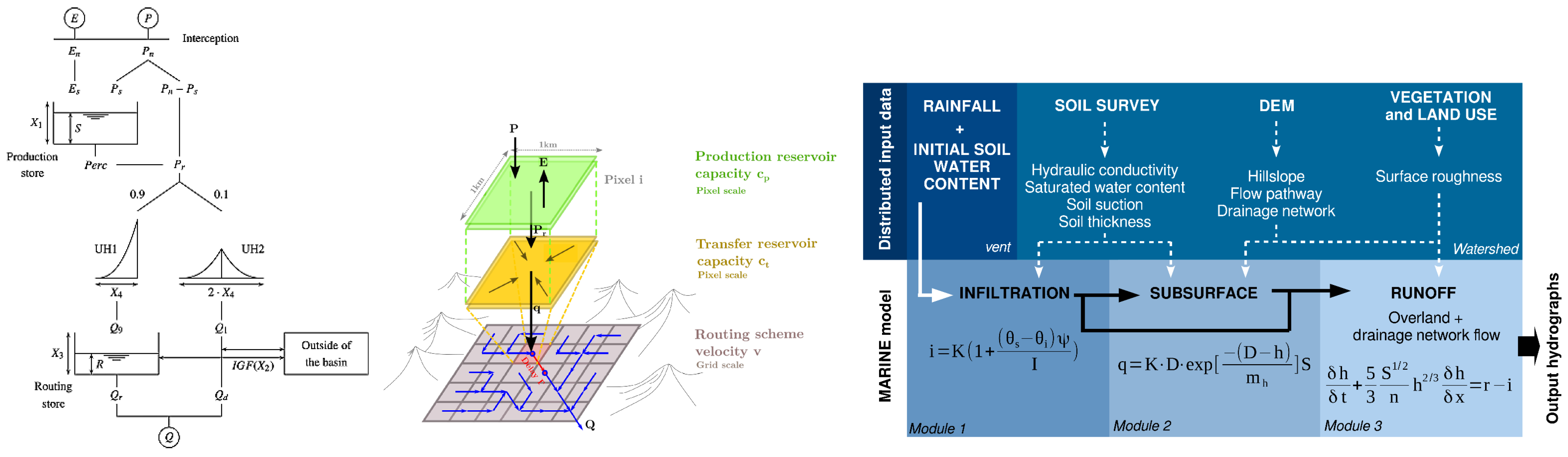
We consider three hydrological models of varying complexities; GR4H, SMASH, and MARINE. The models are shown in
Figure 1, and their description is given in
Table 1. Here, we present their general formulations, but the details of the modeling operators are given in
Appendix A. Note from
Table 1 that the MARINE model is used with a finer spatio-temporal resolution compared to SMASH. This has a limited impact on the results since all models are forced with the same rainfall data (spatially averaged to the catchment scale in the case of the lumped GR4H model).
We considered a 2D-spatial domain (catchment) covered by a regular rectangular grid of resolution (in the case of the distributed models). The unique constraint applied to this lattice is that a unique point has the highest drainage area, that is the catchment outlet, given the flow directions. The time is denoted . The spatio-temporal rainfall and evaporation fields are, respectively, P and E, and stepwise approximations over time steps are assumed.
2.1.1. GR4H Model
The GR4H model [
32] is a lumped continuous model, i.e., taking as the input the spatial averages over catchment domain
of the rainfall
P and evaporation
E fields at each modeling time step (hourly), and based on the GR4J model formulation of [
37].
The partition of the input neutralized rain
(cf.
Appendix A.1.1) is performed between an infiltration part
filling the production reservoir of maximum capacity
and an effective rainfall
flowing into the transfer components. The production function is the classical GR production function [
38], described in Equation (
A1). The splitting of the effective rainfall takes into account quick and slow flow components. Ten percent of the effective rainfall
resulting from the excess of the production and the percolation is routed linearly using a unit hydrograph UH2 of time base
, and the remaining 90% is initially routed using UH1 of time base
, then using a nonlinear routing store of reference capacity
. The ordinates of the UH are derived from their respective S hydrographs, which also are functions of
. A groundwater flow exchange term
F from the reservoir, which depends on both the actual level in the routing store
the reference level of the nonlinear routing store
, and a water exchange coefficient
, is taken into account in both flow components. Finally, the total stream flow
Q is obtained as the sum of the resulting flows from the routing reservoir
and the output of UH2
.
This model has been used in many studies such as flash flood modeling in four tropical mountainous watersheds in New Caledonia [
39], for testing the transferability of the GR4H model parameters for extreme events on the Mediterranean island of Cyprus [
40], or for the comparison of two satellite-estimated precipitation products in hydrological simulations in Rimac Basin, Peru [
41], among many others.
2.1.2. SMASH Model
Spatially-distributed Modeling and ASsimilation for Hydrology (SMASH) is a computational software framework dedicated to spatially distributed continuous hydrological modeling including variational data assimilation [
13]. We used the 3-component model (production, transfer, routing) from [
13]. For a given pixel
i of coordinates
, two reservoirs
and
, of capacities
and
, are considered for simulating, respectively, the production of runoff and its transfer within a cell. Their stages are, respectively, denoted
and
. The runoff amount is then routed between pixels. The partition of the input-neutralized rain
(
Appendix A.1.1) between an infiltration part
filling the production reservoir and an effective rainfall
filling the transfer reservoir is performed with a production operator. In this study, a Green and Ampt infiltration model (Equation (
A3)) enabling simulating ponding when the rainfall intensity exceeds the infiltration rate is implemented and used in the model. The production reservoir is then emptied from the actual evaporation
calculated with a “GR” evaporation operator (Equation (
A2)).
The effective rainfall after production is transferred within a pixel through a conceptual reservoir of maximum capacity
(Equation (
A4)), while routing is performed with a linear unit Gaussian hydrograph, whose delay
from node
to node
i is controlled by the routing velocity
v and the distance
between the cells. The model formulations are described in
Appendix A.1.
2.1.3. MARINE Model
MARINE is an event-based, physically based, parsimonious, and fully distributed model designed for flash flood prediction based on the supposedly main hydrological processes involved in Mediterranean catchments. These processes include infiltration, subsurface runoff, overland flow, and flow in the drainage network. On the contrary, evaporation and deep percolation are considered negligible at the event scale, and therefore not represented. It was borne out of the need to address the peculiarities identified by Roux et al. [
20] MARINE being an event-based model, the local infiltration function used is a typical event-based model, accounting for the infiltration at the local scale and described by the Green and Ampt model (Equation (
A3)). The surface runoff is divided into overland flow and drainage flow; in both cases, the kinematic wave model was used assuming a 1-dimensional kinematic wave, which is approximated with the Manning friction law, while the subsurface flow is based on Darcy’s law. The model formulations are given in
Appendix A.1.
The input data were sourced from the information of surface topology, soil survey, vegetation, and land use, and the model was initialized using the soil moisture outputs of the SIM model.
The spatial resolution was set to m2, and the fixed simulation time step was set to min (Courant–Friedrichs—Lewy (CFL) check and automatic temporal sub-iterations if needed for kinematic wave resolution), i.e., finer than the rainfall space–time resolution.
2.2. Calibration Procedure
The objective of the calibration was to search for an optimal (in a sense to be defined) set of parameters that reduces the discrepancy between simulated and observed discharges at a catchment outlet. The calibration procedure was integrated inside each model. Note that these methods differ, but we supposed them to be specifically designed for each model and available to the end-user. In fact, developing a calibration procedure is a delicate task, and thus, the bias introduced by these calibration methods will be considered as a model’s weaknesses.
The objective function used for calibration is based on the classical NSE efficiency (given in
Section 2.4.4), which is adequate for the present flood modeling context. For all models, considering
, a quadratic discrepancy measure between simulated and observed discharge,
and
, the parameter calibration inverse problem reads:
where the cost function
J depends on the sought model parameter vector
through the hydrological model response—i.e., the simulated discharge
with
the atmospheric inputs of a hydrological model
whose internal states are
. For each model, bound constraints were applied on the sought parameters using the same ranges as in the sensitivity analysis (cf.
Section 2.4).
2.2.1. GR4H
For the GR4H model, four parameters, described in
Section 2.1.1, were optimized (see
Table 2). They are the production storage capacity
, groundwater exchange coefficient
, max. capacity of the routing store
, and time base of the unit hydrograph
. The calibration was performed using the Michel calibration algorithm [
37,
45], which starts with random starting points in the parameter space, and then, the optimum search is performed with a simple descent method.
2.2.2. SMASH
In the case of this model, we used the variational algorithm presented in [
13] for the calibration of the parameters. The algorithm enables the calibration of spatially distributed model parameters (high-dimensional optimization problems), under various constraints. It starts from a spatially uniform prior guess on the sought parameters. This prior guess is obtained with a simple global calibration algorithm, as in [
13]. The minimization of the cost function is then performed using the Limited memory Broyden–Fletcher–Goldfarb–Shanno Bound-constrained (LBFGS-B) descent algorithm [
46], making use of the gradient of the cost function, which is obtained from the adjoint model thanks to the Tapenade automatic differentiation engine [
47].
However, using only downstream integrative discharge for calibration leads to well-known equifinality issues in spatially distributed hydrological modeling faced with overparameterization. We, therefore, reduced the control space by grouping the sought parameters into classes through the application of spatial masks, which we derived from prior physiographic information (following [
34]). For example, in the case of Gardon, have a size of 543 km
2 hence 543 pixels of 1 km
2, instead of calibrating (
parameters), we applied a physiographic mask for each parameter. If the mask for the routing parameter
v has only two classes (one for the drainage network and another for the hillslope), only two
v parameters will be optimized (instead of 543 pixel values).
A key task is to find relevant spatial information to define the mask for the parameters of a model that is conceptual (SMASH). In Jay-Allemand [
34], different masks were proposed and tested. However, for the present intercomparison study, we used the same physiographic maps that we used for the MARINE model. They are summarized in
Table 3.
At the end, four free parameters
and
times their respective number of classes defined by their masks (see
Table 4) need to be calibrated. Suction
and porosity
were not calibrated based on the previous sensitivity analysis of the Green and Ampt model in a similar context [
20,
22]. While we constrained
using prior soil information (
Table 3), we kept
simply at a value of 1 (see
Appendix A.1.2). In the rest of the article, we call this calibration method from [
34] “masked” calibration.
2.2.3. MARINE
This model requires only five parameters to be calibrated for the whole catchment; see
Table 5. The first three are the correction coefficients applied to the distributed maps of saturated hydraulic conductivity
, the soil thickness
and the soil lateral transmissivity
. The last two are Manning–Strickler’s friction coefficient for the river bed
and for the flood plain
. These correction coefficients were applied during the calibration process such that the absolute values of the parameter in question were modified while the spatial pattern as sourced was preserved.
The optimization algorithm in the case of this model is based on a gradient-based descent algorithm, Broyden–Fletcher–Goldfarb–Shanno (BFGS), from multiple starting points [
20]. The gradient was evaluated by finite differences.
2.3. Study Area and Data
In this section, we begin by presenting the two study catchments, then we present the various data we used, as well as their sources.
2.3.1. Catchments
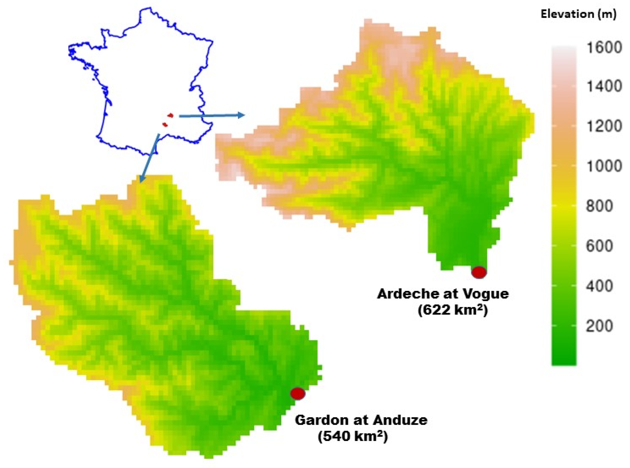
The two study catchments (Gardon at Anduze and Ardeche at Vogue) are located in the Cevennes region (see
Figure 2). They are prone to flash floods and are influenced by a Mediterranean climate. There is strong seasonality of rainfall runoff in both catchments. Summer is the driest season with the flow at the lowest level. Autumn receives the highest rainfall and the seasonal flow is the largest, especially in the month of November. Much higher rainfall and runoff occur in the two other seasons of winter and spring compared to summer. The two catchments can be considered as undisturbed without significant anthropogenic impact on their hydrological responses. Their description is given in
Table 6.
Gardon, with its outlet at Anduze, drains an area of 540 km
2. It is well gauged and has a Mediterranean climate. Autumn is characterized by the occurrence of flash floods and the highest rainfall intensities, while summer is mostly hot and dry (see Roux et al. [
20]). The catchment geology is mainly dominated by a fractured metamorphic formation, classically the schistose; however, there are some karstic zones around the junction of Saint Jean and Mialet [
42]. It has a highly marked topography consisting of high mountain peaks, narrow valleys, and steep hill slopes. The vegetation is dense and composed mainly of beech, chestnut trees, holm oaks, and conifers [
49]. The elevation varies from 129 m at Anduze to 1202 m at the highest point. The average slope of the basin is about 20%, but can be up to 50% at the upstream. The soil (made of silty clay loam and sandy loam) has a mean thickness of around 28 cm and a mean saturated hydraulic conductivity of 5 mm/h.
The Ardeche catchment at Vogue drains an area of 622 km
2 and is exposed to intense precipitation events due to the convection of humid sea air masses over the Cevennes mountain slopes [
23]. It presents a mixed geology, with metamorphic rocks and schist on the upper part of the catchment and sedimentary plains downstream. The land cover is mainly mixed forest, natural grasslands, and shrubs. The elevation varies from 1530 m at the upstream to 150 m downstream. The depth of the soil in the catchment ranges from as low as 5 cm to as deep as 50 cm with an average depth of 28 cm. The soil texture is mainly sandy loam with silt deposits downstream. The mean saturated hydrological conductivity is around 8.6 mm/h.
2.3.2. Data
This section describes the various data used in the study. For a fair assessment of the models, the same input of rainfall and, for the specific case of the continuous models (SMASH and GR4H), potential evapotranspiration (PET), were used:
Discharge: Observed discharges at gauged outlets of Vogue (Ardeche) and Anduze (Gardon) were used for model calibration and validation. Discharge series were extracted from the national banque hydro (
http://www.hydro.eaufrance.fr/, last access: 10 March 2021).
Rainfall: We used rainfall data from the radar observation reanalysis ANTILOPE J+1, which merges radar and in situ gauge observations. These data are provided by Météo-France. Rainfall averages were used as the input for the 3 models depending on the grid resolution, in this case, a grid of 1 km2 for the distributed models (SMASH and MARINE) and a spatial average at the scale of the catchment size in the case of the lumped model (GR4H).
Potential evapotranspiration (PET): The interannual temperature data were provided by the SAFRAN reanalysis and then used to calculate the potential evapotranspiration using the Oudin formula [
50]. PET is at the same resolution as the rainfall data. These data are specific to the continuous models (GR4H and SMASH).
Physiographic data: The soil thickness and texture maps were derived from the surveys provided by the INRA and BRGM. Soil classes and, consequently, the suction, porosity, and saturated conductivity were derived from the soil texture using the Rawls and Brakensiek relations [
48]. The vegetation and land use from the 2000 Corine Land Cover provided by the Service de l’Observation et des Statistiques (SOeS) of the French Ministry of Environment (
www.ifen.fr) were used to derive the surface friction. These are exactly the same data used and sourced from Roux et al. [
20]. The resulting maps were used as the inputs for the MARINE model to provide physical operator parameter values, while they were used as mask inputs for the SMASH model in the calibration by classes (masked calibration) (refer to
Table 3).
Soil moisture data: SAFRAN-ISBA-MODCOU (SIM) [
35] is an operational modeling chain that simulates both the flow of water and energy at the surface, as well as the flow of rivers and major aquifers. It is forced by the atmospheric reanalysis from SAFRAN and uses ISBA to simulate the exchange of water and energy between the soil and atmosphere and MODCOU as the hydrological model.
We used two versions of the SIM model: SIM1 and SIM2. The first version, SIM1, uses the force-restore version of ISBA, ISBA-3L [
51,
52], in which the soil is discretized into three layers corresponding to the surface, root, and deep zone. SIM2, on the other hand, uses the diffusive version of ISBA, ISBA-DIF [
53], with a vertical soil column discretization into a maximum of 14 layers. In the case of this study, the humidity of the root zone was considered as the sum of the humidities of the layers between 10 cm and 30 cm deep. The two outputs (SIM1 and SIM2) available for this study are at a daily time step (06 UTC) and a spatial resolution of a 8 km square grid.
We used SIM1 simply for the initialization of the MARINE model, as was done by several authors (see [
15,
21,
23,
43]), while we used SIM2 as the benchmark to compare the simulated soil moisture outputs of the three study models: SMASH, GR4H, and the MARINE model.
2.4. Methodology
This section presents the numerical experiments we performed to answer the research questions that we raised. The first experiment was to investigate the global sensitivity of the three models. The second experiment was aimed at the calibration and validation of the models using a split-sample procedure. The last experiment compares the model performance and signatures at the event scale. We also briefly present the evaluation criteria we used to compare the models.
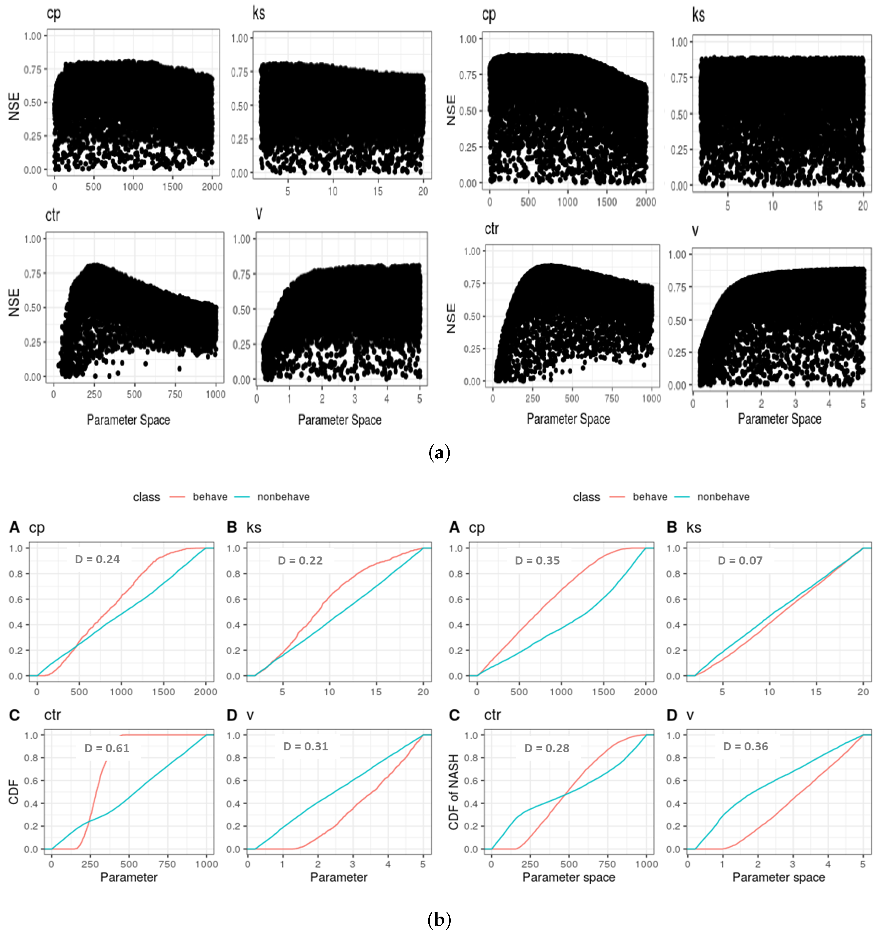
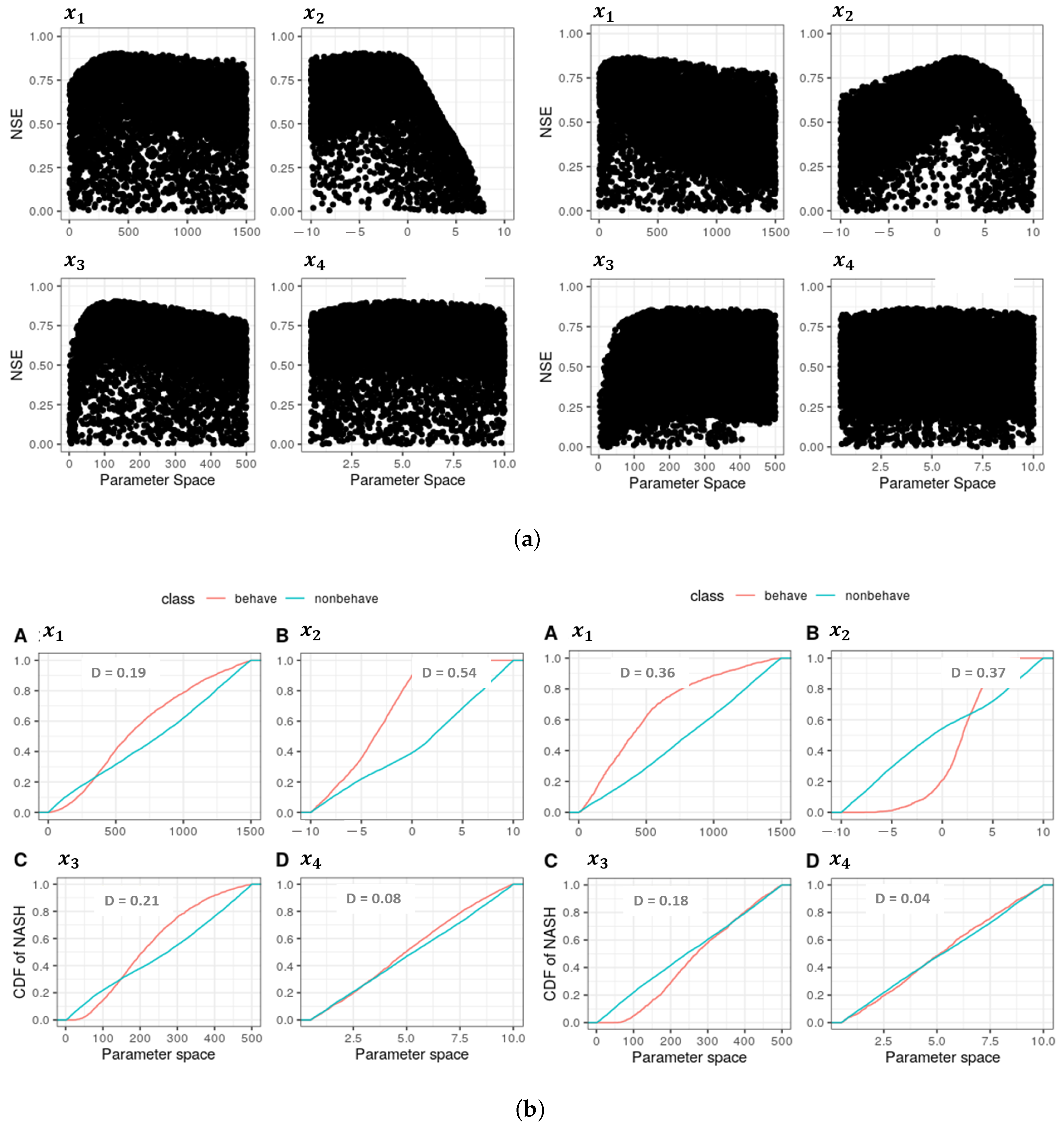
2.4.1. Regionalized Sensitivity Analysis
We used regionalized sensitivity analysis (RSA) to conduct the global sensitivity analysis of the parameters of the models. For the details of this method, see [
54] and the references therein. The idea is to compare the sensitivity of the parameters responsible for the vertical and lateral water partitioning within the compartments of each model studied.
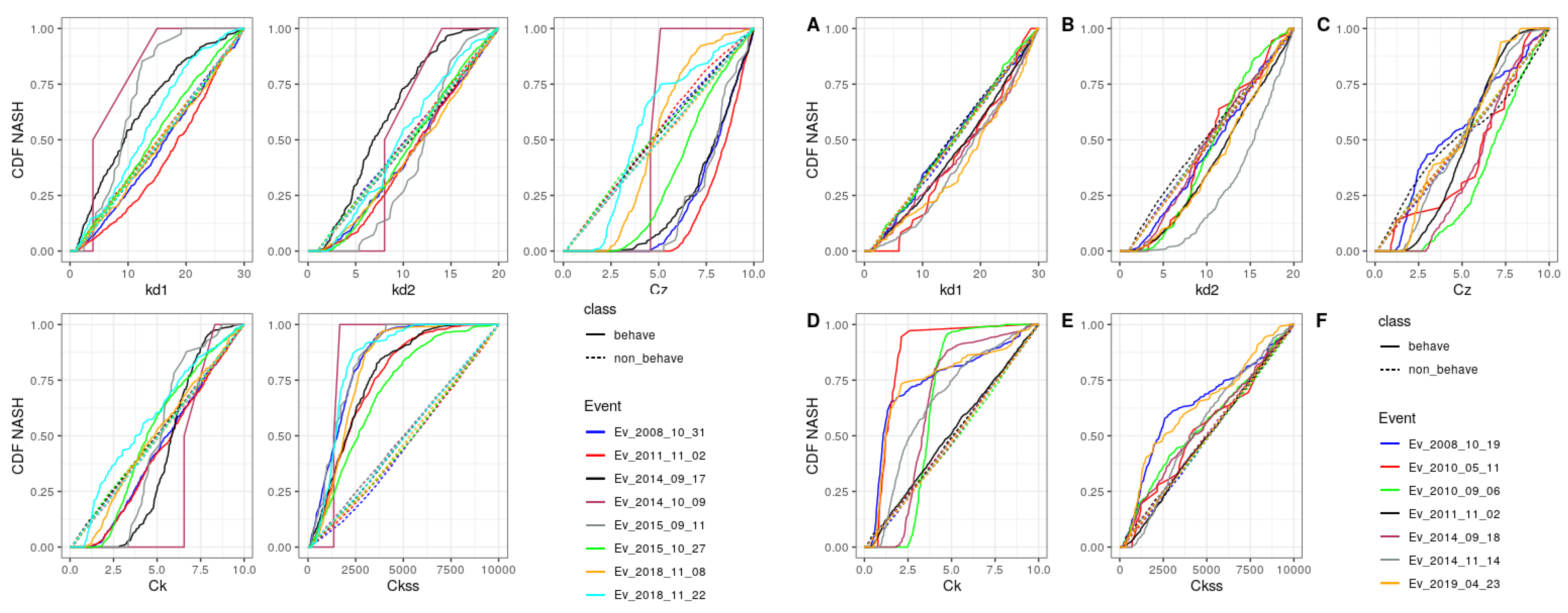
We performed 10,000 Monte Carlo simulation runs, while sampling the parameters assuming a uniform distribution. We used the threshold of 0.7 NSE (Equation (
1)) for the classification of the runs into the behavioral (runs with NSE ≥ 0.7) and non-behavioral (NSE < 0.7) groups. As noted by Beven [
10], the KS test can be very sensitive to small differences and will thus report significant differences between the two classes. Hence, the magnitude of the KS statistics
D, representing the maximum difference between the cumulative distribution functions (CDFs) of the two classes, was used to rank the parameters based on their sensitivity.
First, in the case of the GR4H model, which is lumped, we investigated the four parameters,
x,
x,
x, and
x, within the range given in
Table 2.
Secondly, in the case of the SMASH model, which is a fully distributed model at a spatial grid of 1 km2, classical reduction of the high-dimensional control space was adopted. The parameters of the model were taken as being spatially uniform, and therefore, the RSA was performed assuming one parameter set at a time for the whole catchment considered. The four parameters were: and .
Lastly, the sensitivity of the five MARINE model parameters (see
Table 5) was investigated. Being an event-based model, we conducted the RSA individually on each of the selected events (
Table 7). A similar approach was followed by [
20,
33]. Unlike the case of [
33] and the references reported therein, where the result of the sensitivity analysis was used to choose calibration/validation events, our methodology here is basically to investigate the parameter sensitivity. The method for the choice of the calibration/validation events is described in
Section 2.4.2.
2.4.2. Calibration and Validation
We calibrated each of the three hydrological models, GR4H, SMASH, and MARINE, with their dedicated methods presented in
Section 2.1. The methods enabled adequate calibrations for each model, as will be presented later in
Section 3.2.
In order to perform fair comparisons, considering a comparable amount of hydrological information learned by the models in the calibration phase, we performed the calibration and validation using the split-sample test procedure [
55], which involved dividing the data into two subperiods. We considered a time series of 13 years at an hourly time step, and we divided it into two subperiods of 7 years each for the calibration and validation. Period 1 is defined from 1 August 2006 to 1 August 2013, while Period 2 is defined from 1 August 2012 to 1 August 2019. Calibration was performed first using Period 1 and then validation on Period 2; the reverse was then performed, in which Period 2 was taken as the calibration period, while Period 1 was taken for validation.
For each calibration period, we used 1 year as the warm up period to initialize the continuous models, which is adequate for hydrological models, as reported by Kim et al. [
56]. In the case of MARINE, we classified the events (see
Table 7) into the two periods (similar to the continuous models) and conducted a multi-event calibration and cross-validation. This multi-event calibration of MARINE was proposed in Garambois et al. [
21]. For all the calibrations, we used the NSE as the objective function.
2.4.3. Comparison at the Event Scale
We designed this experiment to compare the three models for flash flood modeling; hence, we selected specific flood events of a return period higher than 2 years within the period of 13 years (2006–2019) for both catchments. These events, described in
Table 7, provide distinct characteristics in terms of the flood peak magnitudes, the volume of water exported, the number of peaks, the gradients of the rising and falling limbs, as well as the spatial and temporal patterns of the underlying precipitation events. Return periods were obtained by fitting the generalized extreme value (GEV) to the annual maxima.
First, we assessed the performance of reproducing the outlet discharge using the NSE criterion, the percentage peak difference (PPD), the peak delay (PD), as well as the synchronous percentage of the peak discharge (SPPD). These criteria are introduced in
Section 2.4.4.
Secondly, the “soil moisture” simulated by the models was compared with the outputs of the SIM2 model. We started by taking the spatial average at each time step, since the models are at different spatial resolutions (SIM2 outputs at 8 km2, SMASH and MARINE at 1 and 0.5 km2, respectively, and lumped GR4H at the scale of the catchment size). We then compared these spatial averages at each time step with those of the SIM2 outputs, which in our case was the reference benchmark.
2.4.4. Performance Evaluation Criteria
In the course of all the calibration and validation of the hydrological models used, the objective function used for the calibration is the widely used Nash and Sutcliffe efficiency criterion, which puts more weights on the high flows than on the low flows and is adapted to our objective of assessing the ability of the model to simulate flash floods.
where
is the mean of observed discharges and
are simulated and observed discharges at time step
i, respectively.
For the case of inter-model performance evaluation between SMASH, GR4H, and MARINE at the event scale, we used other criteria. These included:
The Kling–Gupta efficiency (KGE) [
57], which provides an alternative to the NSE and gives balance to the correlation, flow variability, and water balance.
, the Pearson correlation coefficient, evaluates the error in the shape and timing between observed () and simulated () flows; is the co-variance between the observation and simulation; is the standard deviation; evaluates the bias between the observed and simulated flows, where is the mean. , the ratio between the simulated and observed standard deviations, evaluates the flow variability error.
Percentage peak difference: This criterion is given as and is used mainly to judge the percentage of the observed peak predicted by the model; the duo must not coincide with the time of occurrence.
Peak delay (PD): This is given as and simply computes the difference in the time or delay between the simulated and observed peak in hours.
A more rigorous criterion in terms of safety is the synchronous percentage of the peak discharge (SPPD), which accounts for the ratio of the estimated discharge and observed discharge at the time of the observed peak discharge. It was used first by Artigue et al. [
58] and, then, subsequently by Jay-Allemand et al. [
13], and it can be written as
Finally, we also used as a metric a comparison of the observed and simulated runoff coefficient (CR) at each event.
3. Results and Discussion
The results obtained are presented here, along side relevant discussions. We start by summarizing the RSA results, followed by the calibration and validation efficiencies. Then, we present and discuss the event signatures for each model and, finally, the results of the comparison of the simulated soil moisture.
3.1. Sensitivity Analysis Summary
Table 8 and
Table 9 give the parameter sensitivity ranking of the three models according to the Kolmogorov–Smirnov test statistics
D (see
Appendix B for detailed results). In the case of Gardon, the parameters of the model that affect the transfer are sensitive (
for SMASH;
for GR4H;
for MARINE). Ardeche, on the other hand, has parameters that affect the production components of the model as generally sensitive (
for SMASH;
for GR4H;
for MARINE). Note that
, the non-conservative exchange parameter of GR4H, was found as the most sensitive for both catchments.
3.2. Calibration and Validation
3.2.1. GR4H
In the case of the calibration of the GR4H model on the two catchments, the parameters and efficiencies obtained both in calibration and validation are shown in
Table 10. All calibration and validation efficiencies were higher than 0.7. In the case of Ardeche, there was stability/robustness in the calibration and validation efficiencies. The groundwater exchange coefficient
was positive in both calibration periods for Ardeche, while it was negative in the case of Gardon. According to this model, positive values show water import, while positive values indicate water export.
3.2.2. SMASH
The result of the mask calibration of the SMASH model parameters is given in
Table 11 for the two study catchments.
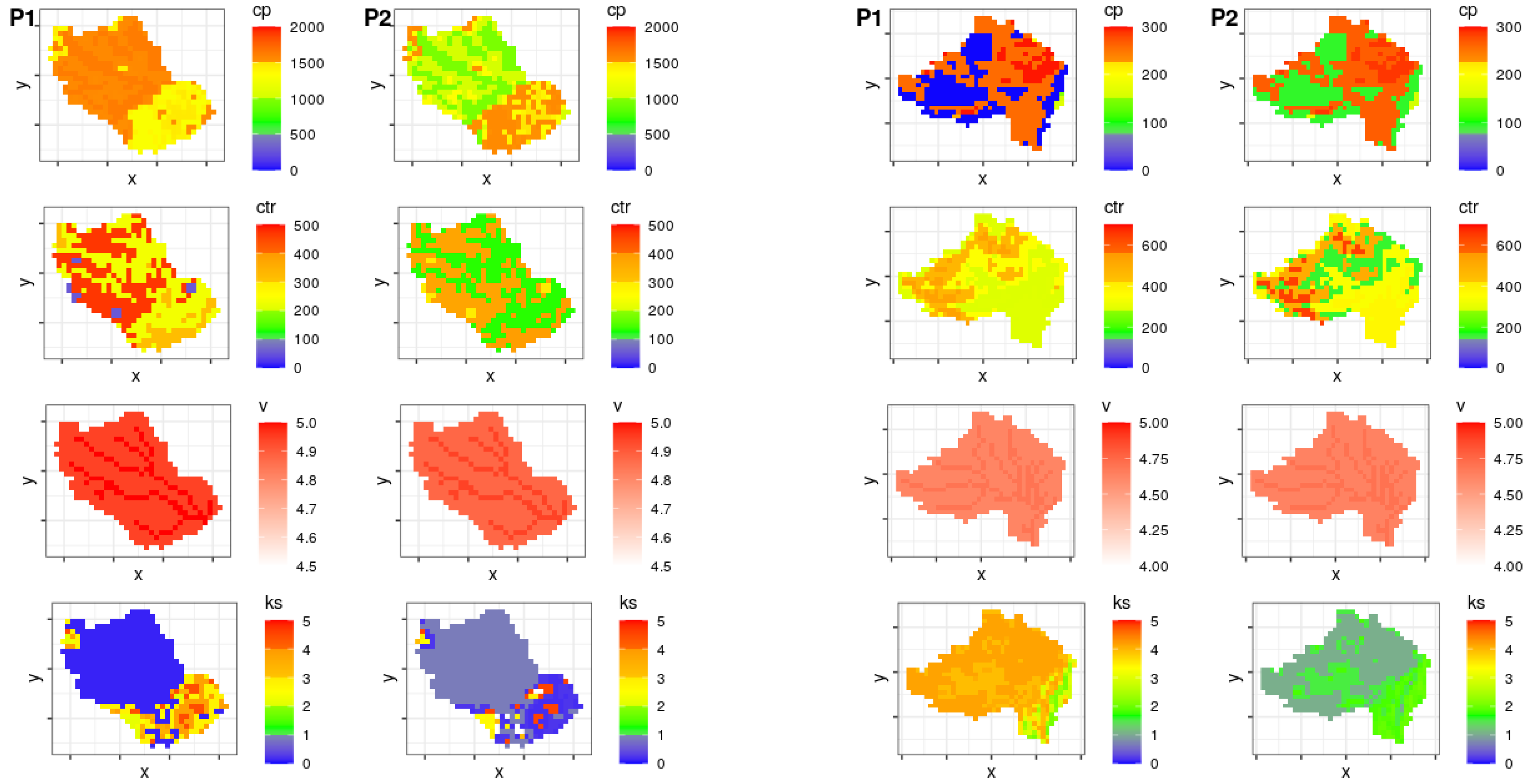
The class-by-class (mask) calibration efficiencies for the two periods varied for the two catchments, but both were more than 0.7. The resulting temporal validation efficiencies were also high. Ardeche presented better calibration/validation efficiencies than the Gardon catchment. The maps resulting from the calibration are given in
Figure 3 for both periods (P1 and P2), and their summaries are given in
Table 11. The results for Gardon (left) show that the calibrated reservoirs’ capacities
and
changed in magnitude with the calibration period (both were smaller in Period 2), whereas the routing parameter
v remained fairly stable (as found in Jay-Allemand et al. [
13]). The converse was true in the case of Ardeche for
and
. The
parameter, however, decreased in Period 2 for both catchments. Jay-Allemand et al. [
13] observed the same difference while studying the Gardon catchment under a fully distributed calibration and concluded that the differences were a result of different rainfall patterns between the two periods, rather than from the calibration algorithm.
3.2.3. MARINE
The resulting global efficiencies are presented in
Table 12 for both catchments. Event-specific NSE (not shown here) had an average of 0.87 and 0.78 for the Gardon events of Period 1 and Period 2, respectively.
The Period 1 and Period 2 events of the Gardon catchment resulted in very similar values, except the parameter, which was almost twice in Period 1 compared to Period 2. For Ardeche, higher calibration efficiencies were obtained compared to Gardon, although the parameters between the two periods were dissimilar.
Validation efficiencies in terms of Nash are presented in
Table 13 for both catchments. The efficiencies are event dependent. For Gardon, an NSE as high as 0.91 was obtained and as low as 0.09, with the average of 0.58 for the eight events. The two November 2018 events presenting the least efficiencies had the least observed peak magnitudes (655 and 809) compared to the max of 1356 m
3/s observed with the October 2015 event. It is thus possible that the soil thickness coefficient used (8.0) is too large for these events. In the case of Ardeche, the NSE in the validation is also event dependent; the min/max obtained was 0.47/0.87 with an average of 0.77. Finally, the temporal performance decrease in validation was smaller in Ardeche (from 0.96 to 0.77 on average) compared to Gardon (0.85 to 0.58).
3.3. Comparison at the Event Scale
In this section, the performance of the models at the event scale is compared. This was performed through the signatures of the simulated discharge and the simulated soil moisture of the 13 events presented in
Table 7. While the simulated hydrographs were compared with the observed hydrographs through the computed metrics, the soil moisture was compared to the outputs of the SIM2 model.
3.3.1. Discharge Simulation
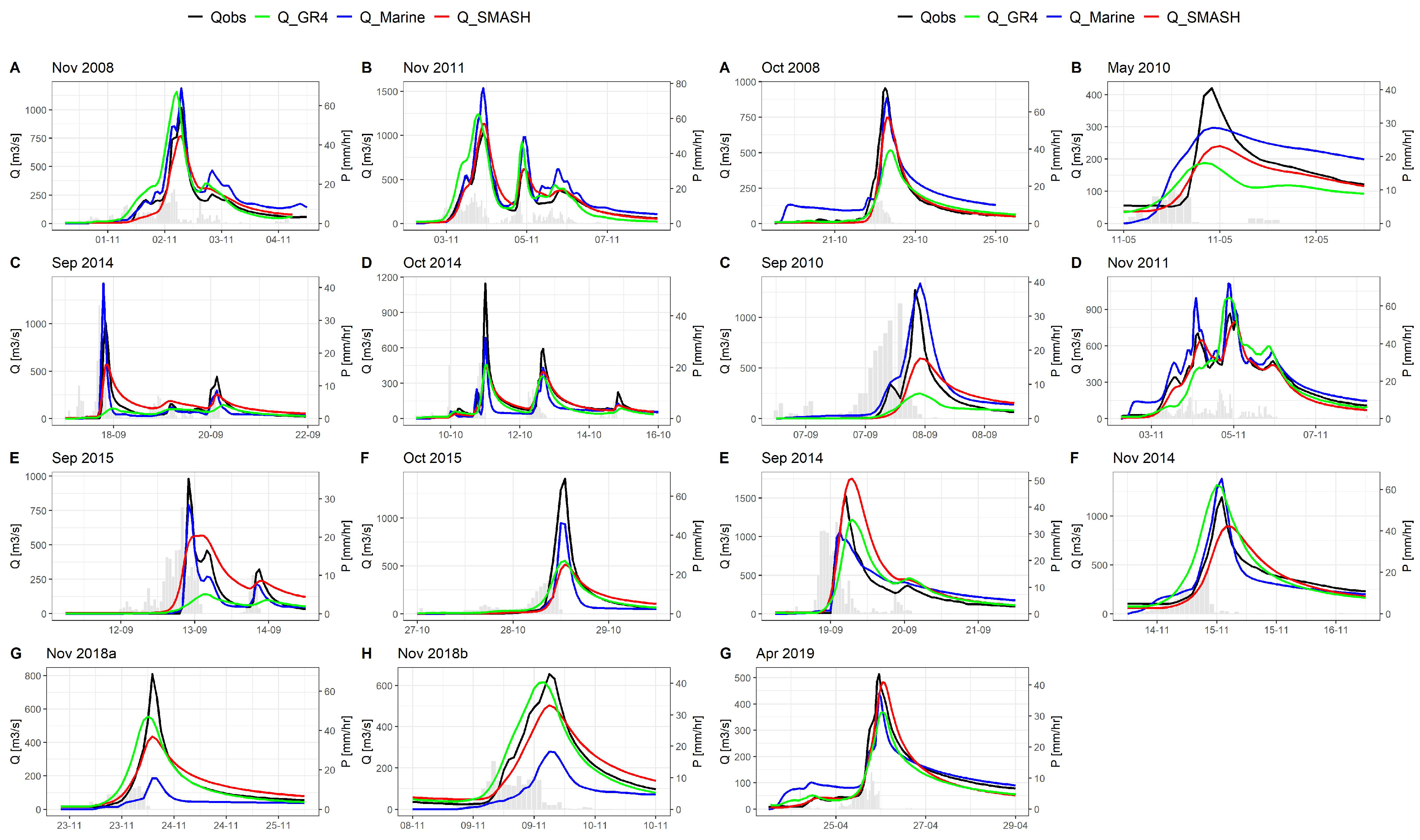
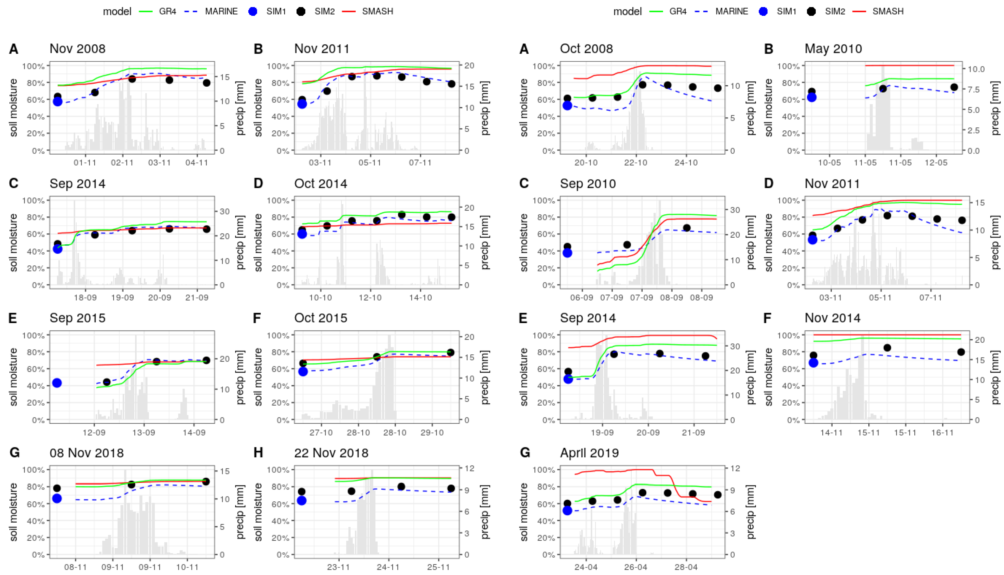
Figure 4 compares the simulated discharges with the three models against the observed discharges for Gardon (left: A–H) and Ardeche (right: A–G). The performance of all the models seems to be fair, and the superiority of the models depends on the event. In order to judge this objectively, different metrics were computed and are shown for both catchments in
Figure 5 and
Figure 6. The performance of the models is therefore judged and discussed according to these metrics in the following paragraphs.
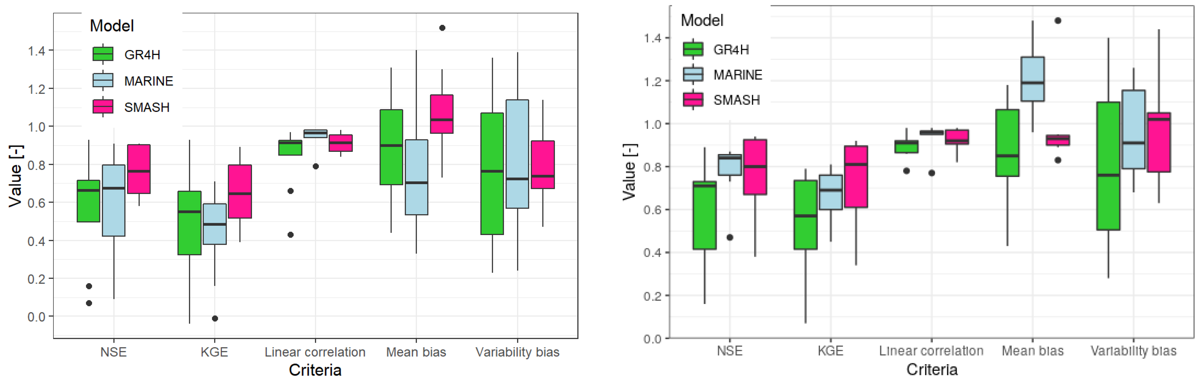
First, looking at
Figure 5, for most of the events in the Gardon catchment, SMASH had better NSE values. The average NSE for the eight events was 0.76 for Gardon against 0.58 for both MARINE and GR4H. For the Ardeche catchment, MARINE was slightly better with a 0.77 average against SMASH with 0.76. GR4H remained the lowest with a 0.58 average. In terms of the NSE, SMASH performed better compared to the other models, while GR4H had the poorest performance.
An alternative to the NSE is the KGE metric. Although the NSE is used in calibration, the KGE criterion is also used to evaluate the performance. This metric gives an aggregated measure of performance in terms of the correlation, mean (water balance), and flow variability bias. Considering Gardon, SMASH had an average of 0.65 against 0.48 for GR4H and 0.44 for MARINE. For Ardeche, on the other hand, SMASH remained better for most of the events, compared to the other models. The average for SMASH was at 0.73 compared to 0.67 and 0.53 for MARINE and GR4H, respectively. Again, for Ardeche, MARINE outperformed GR4H on average.
The three components of the KGE also reveal some relevant information on the performance of the models. In terms of the correlation coefficient r, which assesses the error in terms of the shape and timing of the hydrographs, all the models had high values. MARINE, however, had on average better performance based on this criterion in both catchments (0.94 and 0.96). GR4H had the poorest performance in both (0.83 and 0.89). With this high average, it can be inferred that all the models are capable in terms of reproducing the shape and timing of the hydrographs. measures the bias in terms of the mean (water balance). SMASH has the least bias compared to both catchments (1.08 and 0.99), while MARINE has the highest bias (0.78 and 1.13). Finally, the measure of bias in the flow variability indicates that for most of the events, SMASH has the least bias. On average, however, the bias is the same for GR4H and MARINE.
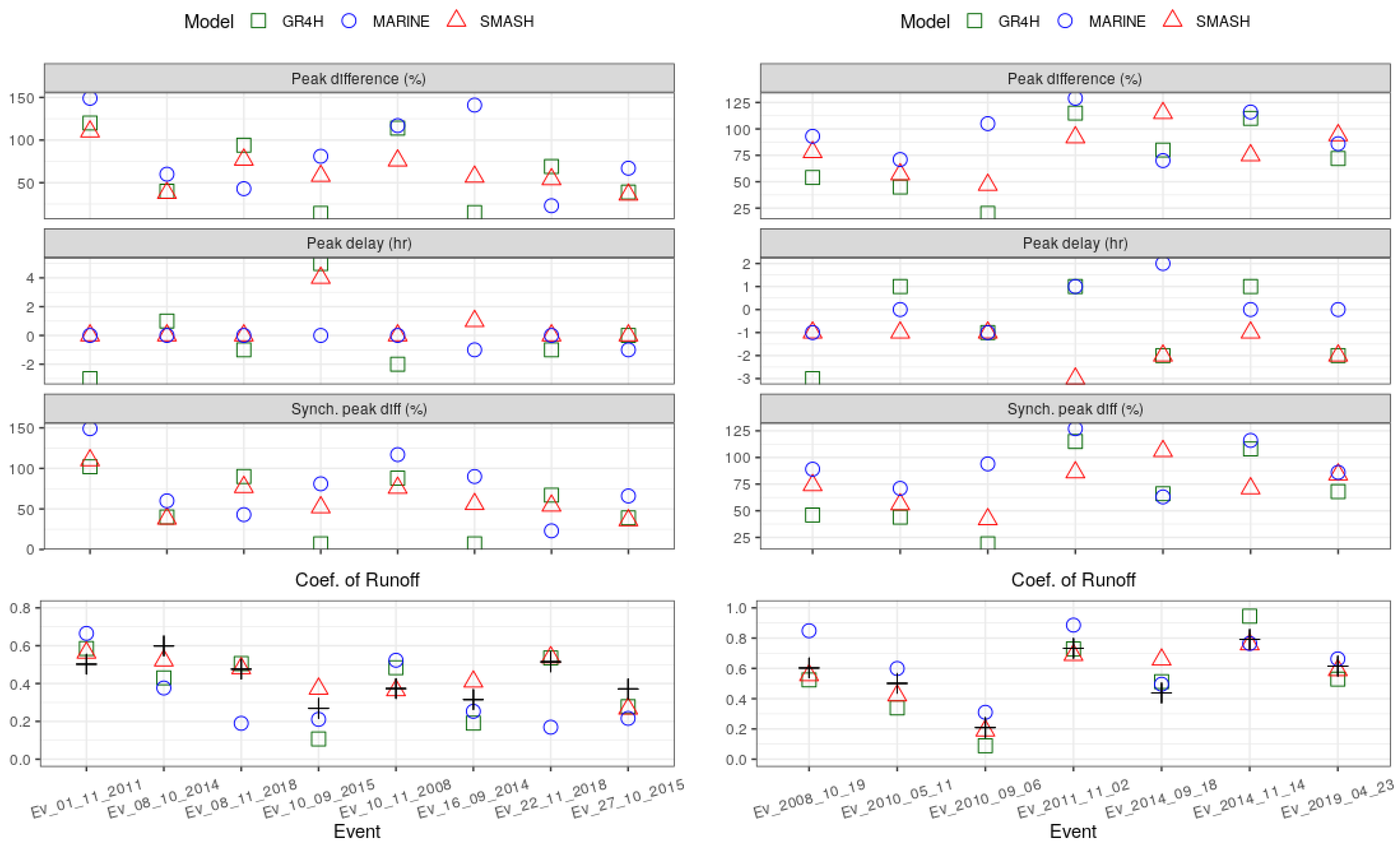
Other indicators to objectively compare the models are shown in
Figure 6 for Gardon and Ardeche, respectively. In terms of the percentage difference in peak magnitude (PPD), the MARINE model approximated the observed peak better than the other models for most of the events in the two catchments. The difference in the timing of the observed and simulated peak was also less observed with the MARINE simulations; SMASH on average had less differences compared to GR4H. The percentage difference between the observed and simulated peak at the time of the observed peak measured by the SSPD criterion indicates more accurate simulations with MARINE. SMASH was yet more accurate than GR4H based on this criterion. This criterion is relevant because it is important to know not only the difference between the observed and simulated peak, but also what peak is simulated at the time the observed peak occurs. Lastly, the runoff coefficient (CR) measures the ratio of the total flow over the total precipitation. SMASH gave the closest CR to the observations for most of the events in the two catchments compared to the other models; it was also the closest to the observations in terms of the average of the CR for both catchments. GR4H closely followed, while MARINE was the least of the two models for both catchments.
Inferring from the results, the event-based MARINE had better performance with regard to the peak simulation and timing, followed by SMASH. However, in terms of the volume of water exported and the water balance, SMASH performed better, followed by GR4H.
Although both the SMASH and GR4H models use the same conceptual production reservoir thickness, the production reservoir in SMASH (used in this study) is filled according to the Green and Ampt infiltration function (infiltration rate equals the rainfall intensity, provided ponding does not occur; when it does, the infiltration excess is transferred). GR4H, on the other hand, is based on the saturation mechanism in which rainfall excess occurs only after saturation. This, in addition to the distributed nature of SMASH, could partly explain why SMASH outperformed GR4H in terms of the indices of peak magnitude and timing. This is despite the fact that GR4H, by construction, has more complexity in terms of processes represented and formulations used, including a non-conservative exchange term (parameter
) (see
Appendix A.1). In terms of the information learned during calibration, MARINE, apart from the physical basis, processes represented, and complexities in the formulations, was simply calibrated over flood events only. The continuous models were, however, calibrated on all the flows (both low and high) and would, therefore, perform better in terms of the volume of the flood.
3.3.2. “Soil Moisture” Comparison
Soil moisture can influence runoff production and is known to be a critical quantity involved in flash flood genesis. Flood models should therefore be capable of performing accurate discharge predictions under dry or wet conditions (see the related analysis of the seasonal flood performances of the lumped GR model, shown to face more difficulties in drier conditions, in [
59]). In this section, we analyze the “soil moisture” variability simulated by the three models.
The spatially averaged time series of the soil moisture predicted by the three models is shown in
Figure 7. In the case of the two distributed models, SMASH and MARINE, the spatial average over the area of the catchment at the hourly temporal scale is shown. The spatial averages of the soil moisture outputs of the two SIM products, SIM1 and SIM2, are also shown. In the case of SIM1, which is used for initialization of the MARINE model, the single value per event (spatial average) corresponding to the beginning of the event is shown, while for SIM2, which is used for comparison, the daily series (available for this study) is shown at 06:00 h of every day for the event duration.
First, the soil moisture output of SIM1 (shown at the beginning of every event) is always lower in amplitude compared to the output of SIM2. While the former discretizes the soil into three layers, the middle layer corresponding to the root zone, the later discretizes into 14 layers, the layers between 10 and 20 cm corresponding to the root zone.
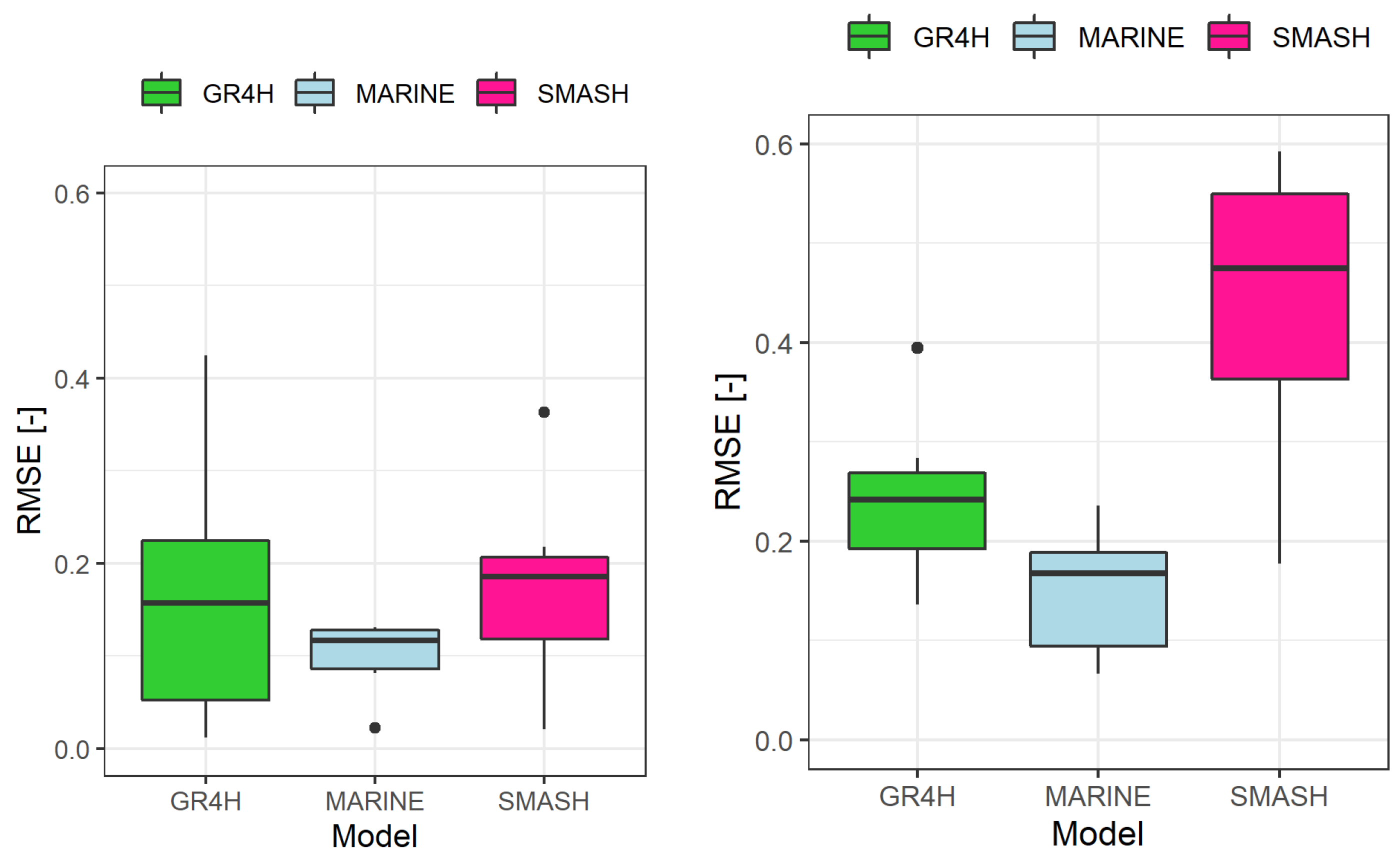
Using the SIM2 series as a benchmark for comparing the three models, MARINE performed best in terms of both the dynamics and amplitude of the soil moisture in both catchments. It was closely followed by the GR4H model, while SMASH had the poorest performance. To assess the goodness of fit between the soil moisture series of the three models in comparison to that of SIM2 (shown in
Figure 7),
Figure 8 summarizes the root-mean-squared error (RMSE) on the eight (seven) events of Gardon (Ardeche), shown on the left and right of the figure, respectively. For both catchments, MARINE was the most accurate (lowest RMSE), followed by GR4H (looking at the median). In the case of Ardeche (right), the 0.75 quantile was lower than the 0.25 quantile of the other two models.
Looking at the SMASH model, we see that in the case of the Gardon catchment, the series remained flat and the response between rainfall events was very weak. Better responses were, however, observed in the case of Ardeche compared to Gardon. This could be possibly explained by the size of the calibrated production reservoir capacity of the two catchments. Large capacities of (1500 and 1200 mm for Periods 1 and 2, respectively) for Gardon against (164 and 200 mm) for Ardeche were obtained. The depletion of the smaller capacity production reservoirs after or between rainfall events would be faster compared to the larger ones. Interestingly, the GR4H calibration resulted in much smaller for Gardon (480 and 230 mm for Periods 1 and 2, respectively) compared to SMASH.
The difference in performance in the soil moisture outputs could be explained by the complexities and processes represented in each of the models. MARINE, in addition to the surface flows (overland and in the channels), subsurface lateral transfers are represented using an approximation of Darcy’s law. Therefore, although evaporation is deemed negligible at the event scale, thus not represented, the lateral flows contribute to the emptying of the soil reservoir and, hence, the faster and sharper decline between and after rainfall events. In addition to this, being a physical model, soil surveys are used as the basis for the soil depths (corrected by a multiplicative factor
). This makes the process and soil moisture variation potentially closer to the real physical phenomena, unlike in the other two models, in which the depths are fully conceptual—and more or less free to vary in space. Recall also that the initial soil water of the event model MARINE is initialized with the outputs of the surface model SIM1, a more complex model with a force-restore approach for modeling soil–plant–atmosphere interactions [
35].
Although both SMASH and GR4H are emptied by the same evaporation function (see Equation (
A2)), the GR4H soil reservoir is also emptied by a percolation leakage. This percolation leakage, although weak, given the power law involved, is an added complexity in the model, which might have resulted in the faster response between rainfall events compared to SMASH. The process of soil emptying of the SMASH (distributed) model is thus more likely to be weaker than that of GR4H (lumped).
In the case of Gardon, the soil saturation of SMASH is generally lower than GR4H for most of the events. This is likely due to the size of the respective production reservoirs (1500 mm for SMASH and 500 mm for GR4H). Apparently, for the same rainfall signal, the soil moisture will be higher in the smaller-sized reservoir. To emphasize, this can be seen in the Ardeche catchment, where SMASH soil moisture was higher for all the events. Interestingly, the production reservoir depth for this catchment was 160mm for SMASH and 300 mm for GR4H. Hence, SMASH saturation was higher (due to smaller capacity). The optimized reservoir depth from the model calibration, therefore, affects the accuracy of the soil moisture estimation.
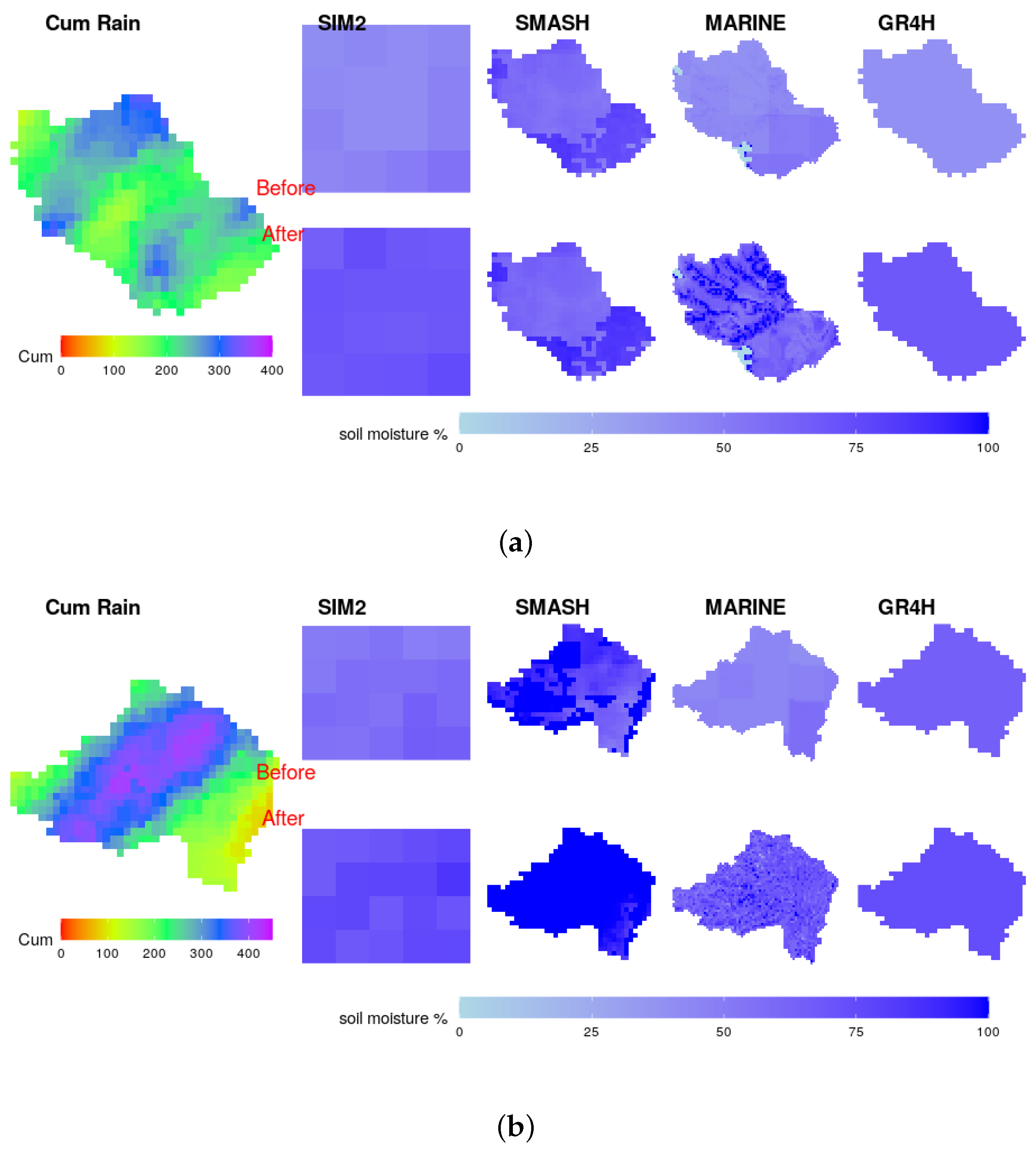
To investigate the temporal evolution of the soil saturation,
Figure 9 presents maps for two chosen events: September 2015 and September 2014 for Gardon and Ardeche, respectively. The figure shows the maps of the cumulative rainfall in mm, the map of the soil moisture in %, for SIM2 (the reference) and those of the three competing models (SMASH, MARINE, and GR4H). For each model, two maps are shown, before and after the rainfall event. The maps reinforce the results seen in
Figure 7: SMASH overestimates the soil moisture before and after the floods. Surprisingly, in the case of the Gardon catchment, at the end of the September 2015 event, different patterns of the soil saturation were observed. While the saturation was higher upstream of the catchment according to MARINE (mostly along the drainage networks), it was higher downstream according to SMASH. This stems from the respective differences between the model calibration methods’ hypotheses, leading to different variabilities of storage capacity patterns. The underlying controllability issue is discussed in what follows.
3.4. Constraints on the Models
The controllability of the models is different: although all three models use the outlet discharge as the variable of interest in the calibration, the MARINE model has constraints on its parameters using field data (soil survey and vegetation and land use), both in terms of their spatial distributions and their magnitude, although the magnitude was corrected using some lumped coefficients during calibration. To highlight these constraints on MARINE, the production reservoir was constrained by the soil thickness map; the Green and Ampt parameters (porosity, hydraulic conductivity, and suction) were all constrained using the soil classes derived from the soil texture. The subsurface transfer was also constrained by the soil classes, and finally, the Manning friction in the kinematic wave routing formulation for overland flow was constrained by the land cover. This gives MARINE more constraints in its parameters, thereby inferring parameters with an imposed spatial pattern and variability from physical maps, as opposed to SMASH. The fact that SMASH uses the same maps during calibration does not offer as much constraint as in the MARINE model. In fact, the use of the maps is only to reduce the high dimensionality resulting from the fully distributed calibration. The constraints are thus applied only on the spatial pattern (via a discretization into a given number of classes), rather than on their magnitudes, as done with MARINE. Again, even the choice of the field data (soil surveys of thickness and texture) to use for the constraint on the spatial pattern of SMASH parameters is not as clear as that of MARINE, since the parameters of the later have some physical meanings, compared to the more conceptual nature of the SMASH parameters. The least constraint applied in terms of spatial pattern is thus on the GR4H model, which is lumped, and thus, relying solely on the outlet discharge in the optimization process. In summary, regarding model parameters’ spatialization, under the tested configurations, SMASH might be overparameterized, while MARINE might be slightly underparameterized.
Lastly, recall that MARINE is also constrained using information from the SIM1 soil moisture output for its initialization at the beginning of each event. With the initial SIM1 controlling the produced flood volume, the MARINE calibration impacts the transfer function more. This might explain why MARINE better reproduced flood peak and timing, but not the runoff coefficient, as shown in
Figure 6.
4. Conclusions
This study aimed at understanding how three models of varying complexities simulated the hydrological behavior of two flash-flood-prone Mediterranean catchments: Gardon at Anduze and Ardeche at Vogue, both located in the South of France. The methodology involved the investigation of the global parameter sensitivity of the models, their efficiencies in calibration and validation, and the assessment of key hydrological signatures at the event scale. Finally, the soil moisture, simulated by the three models at the event scale, which is a critical quantity in flash flood genesis, was compared with the gridded soil moisture outputs of the hydrometeorological SIM model. The three hydrological models were the lumped conceptual model GR4H, spatially distributed conceptual model SMASH, and process-oriented distributed model MARINE.
The invested methodology followed and the results obtained led to the following conclusions:
The results revealed contrasted and catchment-specific parameter sensitivity to the same efficiency measure. Higher sensitivity was found for all models to the transfer parameters for Gardon and for the production parameters for Ardeche. Interestingly, the exchange parameter controlling a non-conservative flow component of GR4H was found to be sensitive.
All three models showed good calibration and validation efficiencies. Their performances were, however, generally better for Ardeche compared to Gardon. In the calibration, MARINE achieved the highest efficiency, followed by GR4H. Although all three models showed a decrease in the efficiencies at the temporal validation, GR4H was more robust. Regarding the parameter stability between the two periods, all the models showed some differences between the calibrated parameters of both periods.
At the event scale, seven events and eight events of contrasted behaviors for Ardeche and Gardon, respectively, were selected to compare the performance of the three study models on the simulated discharge and the soil moisture pattern. The indices of the discharge simulation showed that the event-based MARINE had better performance with regard to the peak simulation and timing, followed by SMASH. However, in terms of the volume of water exported and water balance, SMASH performed better, followed by GR4H.
Using the soil moisture output of the SIM2 model as the benchmark for comparing the simulated moisture by the three models at the event scale, MARINE emerged as the most accurate in terms of both the dynamics and amplitude of the soil moisture in both catchments (recall that MARINE soil water content is initialized with SIM1). It was closely followed by the GR4H model, while SMASH had the poorest performance compared to the other models. The SIM2 product from the SIM model was revealed to be valuable information to assess the internal dynamics of the model states.
Regarding the computational costs, a forward run was relatively inexpensive, even with the considered distributed models, and is feasible in a few minutes of CPU time, while the memory requirement can be larger depending on the size of the spatio-temporal domain.
Overall, we can conclude that the varying degree of complexities in the process representation, constraints applied to the models, the spatio-temporal resolution, as well as the calibration methods in the models appeared relevant in the performance of the models for flash flood modeling. Therefore, considering multiple models for flash flood prediction might be pertinent, as well as improving the process accountancy and versatility of each model, as highlighted by the present study, showing how and why models performed differently. A lumped model might not perform as efficiently as a distributed model in the case of spatialized rainfall flood events (e.g., [
31]), but is generally easier to calibrate compared to distributed models, requiring more constraints regarding spatial overparameterization. Users who wish to apply the studied models, which is feasible from worldwide databases with little preprocessing, are advised to consider the longest rainfall flood time series available in order to enhance parameters’ representativity.
Looking at the process representation, SMASH is the least complex. Recall that while GR4H has a non-conservative water exchange operator revealed as sensitive, MARINE has a subsurface component to account for lateral transfer. The poor performance of SMASH in terms of simulated moisture enhances this aspect. Including either of these in SMASH could stabilize or compensate for the high soil reservoir depth observed for Gardon with this model. MARINE has the finest spatio-temporal resolution, and this, along with the more physical routing model, might have contributed to its fastest reactiveness in terms of the rising limb and peak flow reproduction. This highlights the importance of searching for versatile model structures, in terms of the range of applicability, for contrasting catchments and hydrological processes’ variability, especially under intense rainfalls, which would be well calibrable/regionalizable over large samples.
All models considered in this study would benefit from a calibration–regionalization strategy tailored for applicability to large domains and a large range of flood types and wetness conditions. Improved constraints on the patterns and magnitudes of SMASH parameters, including those of the Green and Ampt model, are required to fully utilize its capacity, especially under intense rainfall events. More generally, reaching higher performances, in terms of flood simulations with a distributed model of increasing complexity, requires developing optimal calibration strategies adapted to overparameterization issues and relying on multisource data, including discharge and physiographic maps, regarding overparameterization issues. Similar remarks were made by Grayson and Blöschl [
12], that these data can help provide information, thereby reducing equifinality and parameter identifiability, which are inherent in complex models. This is even more challenging in a regionalization context and with the will to ensure coherent internal state fluxes. Improved constraints could also stem from flood-specific metrics accounting for multi-frequency signatures.
In terms of perspectives, future comparisons of hydrological models of different complexities should study large samples with rich datasets, including high-resolution satellite data of soil moisture, which are particularly interesting for distributed models, as shown in [
23] for French Mediterranean catchments. One could assess/discriminate internal model behaviors, given multiple plausible parameter sets potentially corresponding to contrasted functioning points, hence model components’ activation/interplay for a given model structure, for instance. Finally, improved calibration–regionalization methods, in a flexible multi-model framework, seem highly needed and will be developed in SMASH with hybrid methods.


 ,
, 


