Article

Evaluation of Long-Term Radar-Derived Precipitation for Water Balance Estimates: A Case Study for Multiple Catchments in Saxony, Germany

Faculty of Environmental Sciences, Institute for Hydrology and Meteorology, Technische Universität Dresden, 01069 Dresden, Germany
*
Author to whom correspondence should be addressed.
Hydrology 2022, 9(11), 204; https://doi.org/10.3390/hydrology9110204
Submission received: 21 October 2022 / Revised: 15 November 2022 / Accepted: 17 November 2022 / Published: 20 November 2022

Abstract

:
Quality of water balance estimations are strongly dependent on the precipitation input. The key limitation here is typically a lack of spatial representation in precipitation data. Quantitative precipitation estimation (QPE) using radar is recognized as capable to significantly enhance the spatial representation of precipitation compared to conventional rain gauge-based methods by calibrating radar pixels with surrounding rain gauges. However, the measured precipitation is often underestimated due to wind drift or funnel evaporation, particularly in mountainous areas. Thus, a post-correction is required before applying radar precipitation in water balance models. Here, we applied the Richter correction for the first time to a radar-based QPE, to model the water balance in ten catchments in Saxony, Germany. The hydrological responses for the period 2001–2017 from the model were validated with discharge observations. The results show that radar data application yielded reliable simulations of water balance (KGE = 0.53 and 0.70 at daily and monthly resolutions, respectively). However, a simple compensation such as the Richter method to conventional precipitation should be used with caution. This study shows that radar-based precipitation has immense potential to advance quality of the precipitation input to distributed hydrologic models not only for flood events but also for climatological analyses.

1. Introduction

Accurate precipitation data is a crucial component in simulating the water balance and hydrologic behavior at catchment scale [1,2]. Many studies have demonstrated that the timing and peak of the simulated response were significantly affected by the spatial resolution of precipitation input to the model [3,4,5]. Rain gauge precipitation data are still referred to as a state-of-the-art data source and are an important input to hydrologic models. The accuracy of flood estimates depends largely on the density of the rain gauge network and the accuracy of the instruments [6,7]. To estimate rainfall over an entire catchment, the point measurements of rain gauges have to be interpolated. As a result, they are limited in their spatial and temporal representation of precipitation [8,9,10]. Inversely, real-time precipitation radar over a large region can provide spatially and temporally high-resolution estimates of precipitation intensity; thus, it is gaining attention in many hydrological and meteorological applications [8,11,12]. However, most applications of radar quantitative precipitation estimate (QPE) are limited to flood or surface water management, and considered typically only for short periods of hours or days or around a flood event [13,14]. Hence, the advantages and possible disadvantages related to long-term radar QPE in water balance modeling, particularly the distinction between accumulated and continuous methods of measuring precipitation, are rather still sparsely considered in scientific research.
Many meteorological institutes around the world, including the German Weather Service (Deutscher Wetterdienst, (DWD)), have used radar QPE to complement rain gauge data [15,16,17]. However, operational radar QPE is a ponderous system and contains many drawbacks such as clutter, spokes, radar rings, or beam blockage, which require many data processing steps to overcome the associated errors in the radar signal. In the last two decades, the DWD has made many advances in deriving QPE from weather radar reflectivity data by developing new algorithms, using consistent processing techniques and integrating more rain gauges for adjustment, and has published a radar climatology dataset, so-called RADKLIM, to support radar-based climatology research [17,18,19]. This dataset is a result of a reanalysis of all their radar data back to 2001, which enables not only heavy rainfall analyses but also another aspect in hydrology study such as water balance components. To the best of our knowledge, an application of this dataset in water balance modelling has not yet been widely conducted in Germany. Therefore, we attempt to investigate the applicability of such radar-based precipitation in water balance models.
As commonly applied in rain gauges that for any water balance calculations, only corrected precipitation values should be used. Despite that the several corrections caused by radar signals were applied, radar data cannot be simply used without processing and corrections [10,20]. In particular, the radar-based precipitation is a product of fitting precipitation values with rain gauge measurements, which leads to an indirect effect of a correction method for rain gauges to radar precipitation values. It is well known that precipitation measurements often result in systematic underestimations due to wind drift and funnel evapotranspiration, particularly at high wind speed, capable of halving the actual rate of precipitation [21]. As a counter measure, several error correction methods were developed, which account for the physical structures surrounding the gauge [22,23]. As a result, correction factors for different countries and different wind shielding categories with seasonal variations are established using simple empirical models. Among them, the “Richter correction” [24] has become a standard procedure to compensate the precipitation measurement with rain gauges in Germany [25,26].
Originally, the DWD’s algorithm in estimating radar-based precipitation is performed by fitting to uncorrected rain gauge data [27]. Thus, here, we test whether application of the Richter method as post-correction on the radar QPE will improve the precipitation input to water balance models. As the Richter correction has been established mainly for rain gauges, applying this correction to radar-based precipitation data is an attempt to conclude on whether this will bring potential benefits for hydrological modelling.
In this study, we used as input precipitation data from radar QPE and traditional rain gauges to the BROOK90 water balance model. The study was conducted in ten small- and medium-sized catchments in Saxony, Germany. We aim to answer the following questions.
How different are the station and radar-derived precipitation for the study sites?
How applicable is radar-based precipitation in water balance modeling?
Does the application of Richter corrections influence the model performance?

2. Materials and Methods

2.1. Study Area

The study is conducted in ten small and medium sized catchments (with the drainage areas ranging from 29 to 131 km2) in the Free State of Saxony, Germany (Figure 1) in the moderate temperate climate zone of Central Europe. Significant regional climate differences can be observed between the catchments. Saxony’s topography from lowlands in the north to low mountain ranges in the south, namely the Ore Mountains, causes a north-south gradient of increasing precipitation [28] and small-scale windward and leeward effects can be observed in the study areas [29]. The average annual temperature (1991–2005) in the northern flat and central hilly part is between 8.5 °C and 10 °C (Figure 1 catchments 1, 2,7, and 9 vs. 3, 4, 5, and 6, respectively), and in the low mountain ranges between 6 °C and 7.5 °C (catchments 8 and 10). Average annual precipitation in the lowlands is 500 to 800 mm (catchments 1, 2, 3, 4, 5, 6, 7, and 9) and about 900 to 1200 in the mountain ranges (catchments 8 and 10) for the same period. The radars in the weather stations Dresden, Ummendorf, and Neuhaus belong to the operational networks of the DWD, and they cover the ten catchments completely. The respective locations, sizes, and land uses of the ten selected catchments are listed in Table 1. The selected catchments represent a variety of different land covers and topographies typical for the study area, without significant anthropogenic influence (i.e., dams, reservoirs, overrepresentation of urban areas).
In addition, there are sensor networks from the DWD (Figure 1) integrated into the open sensor web (OSW; see more details below) used in this study to derive meteorological data. They include, in addition to precipitation rain gauges, other meteorological variables: air temperature, global radiation, relative humidity, and wind speed.

2.2. Data

2.2.1. Dischagre

The observed runoff data measured at the outlet of the selected catchments are available in an hourly resolution and unit m3s−1 provided by Sächsisches Landesamt für Umwelt, Landwirtschaft und Geologie (LfULG). To make the measurements comparable with the output of the model, all values were converted to mm d−1 by considering the catchment area and aggregating discharge to daily values.

2.2.2. Open Sensor Web (OSW)

All precipitation gauges used in this work belong to the DWD network (Figure 1) and were filtered from the Open Sensor Web (https://opensensorweb.de/ (accessed on 20 July 2020)), which incorporates standardized, hourly, and uncorrected measurements. Data from 1 January 2001 to 31 December 2017 were aggregated from hourly to daily resolution to serve as an input for the BROOK90 model. An R package “xtruso” (https://github.com/GeoinformationSystems/xtruso_R (accessed on 10 March 2020)) was developed to facilitate the retrieval and integration of the above-mentioned data sources for meteorological and water balance modeling. By using this package in combination with the abovementioned sensors, daily precipitation and other meteorological variables (global radiation, air temperature, air humidity, and wind speed) can be generated for the BROOK90 model. It follows these steps: (1) Selection of a catchment area using the catchment ID already integrated in the package; (2) Automated extraction of relevant catchment information (e.g., elevation, soil profiles, and land covers); (3) Automated search for in-situ meteo stations in the vicinity of the catchment (maximum of ten stations with a maximum elevation difference of 200 m to avoid orographic effects); and (4) Automated extraction and daily aggregation of measurement time series for the identified in-situ stations.
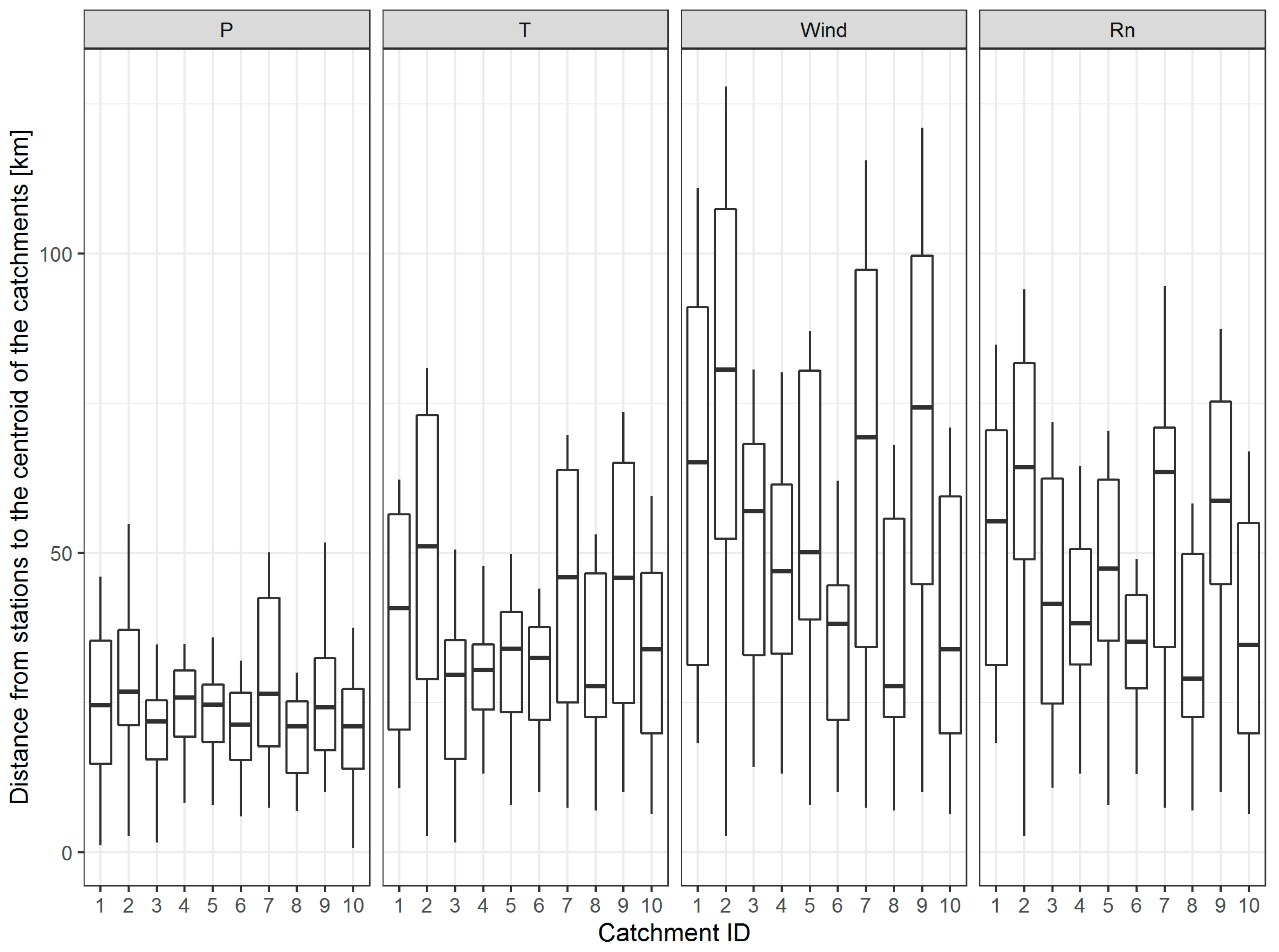
Consequently, the input values for each sub-catchment are estimated from the surrounding measurements using the inverse distance weighting method, which is commonly used for interpolating climate variables [26,30]. The generated time series serve as data input for all hydro response units (HRUs) of the corresponding catchment. In addition, the “raw” precipitation data were also corrected using the Richter method (Richter, 1995). Thus, both versions of gauge data (uncorrected and corrected) were used as inputs to the model. Since each catchment is divided into different sub-catchments based on its topography, the number of stations included in the simulation differs from catchment to catchment (ranges from 50 to 230 stations). In addition, only sensors for humidity and temperature are recorded in the same location, while locations for all other sensors vary. As a result, the distances between sensors and study sites can strongly vary (Figure 2). It should be noted that the longer the distance, the lower is the density of the corresponding sensors considered for the simulation (see detail below).

2.2.3. RADKLIM RW Data Set

The RADKLIM RW dataset is a reanalyzed and temporally extended version of the hourly radar-based QPE product RADOLAN RW fitted to rain gauge data on a nationwide 1-km grid created by the German operational Radar Online Calibration program [17,31]. The dataset is available at the DWD Open Data Portal (https://opendata.dwd.de/climate_environment/CDC/grids_germany/hourly/radolan/reproc/2017_002/bin/ (accessed on 10 January 2020)) and cover the period 2001–2021. Compared to its previous version (RADOLAN RW), the temporal cover was extended from 2006 onwards to 2001 onwards. In addition, several new correction algorithms such as distance and height-dependent signal reduction and spokes, more ground rain gauges, and consistent processing techniques were integrated in the reanalysis process [32]. The data format is reserved like RADOLAN; however, more grid size (1100 km × 900 km) and header information were added in the product. Since its release in 2018, a few tools to assist the comprehensive data processing procedure were developed such as in GIS environment [33] or in R environment with the “xtruso” package (https://github.com/GeoinformationSystems/xtruso_R (accessed on 10 March 2020)). In this study, we carried out the assessment and analysis in R environment; thus, we selected the xtruso package as processing tool and limited the study period to 2001–2017 to cope with the data pre-processing in the package. The raw RADKLIM-RW data provided by DWD need to go through four steps before they can be used in the model (see Appendix A).

2.3. Hydrological Modelling

2.3.1. The BROOK90 Model

The BROOK90 water balance model is based primarily on mass and energy conservation laws to provide a detailed representation of vertical water fluxes within the soil-water-plant system at a single site [34]. Meteorological measurements such as air temperature, humidity, radiation, wind speed, and precipitation at daily resolution are required to run the model. The BROOK90 model simulates daily evapotranspiration using the Shuttleworth-Wallace approach and water movement in variably saturated and unsaturated matrix flow or macropore flow using Richard’s equation. In addition, runoff generation is produced by different runoff pathways (vertical bypass and seepage, surface flow, and lateral subsurface flow). An overview of the model flowchart can be found in (http://www.ecoshift.net/brook/flowchrt.html (accessed on 1 July 2017)). Since it is a lumped conceptual approach, lateral transfer of water to surrounding downslope areas is not considered. Therefore, greater uncertainties may be present when capturing the spatial variation of lateral water movement in soils. The original BROOK90 was developed by Federer et al., (2003) in FORTRAN and it has been improved since then. In 2019, the model was fully translated into R (https://github.com/rkronen/Brook90_R (accessed on 15 May 2019)), which allows easier integration of the model in a data platform for a direct operation as well as parallelization processes to reduce computation time. The model has been already widely applied in previous studies from single sites to regional or even global scale [35,36,37,38]. The BROOK90 model has been proved to perform well with both local and global datasets and its R version has been used in this study [37,38].

2.3.2. Model Setup

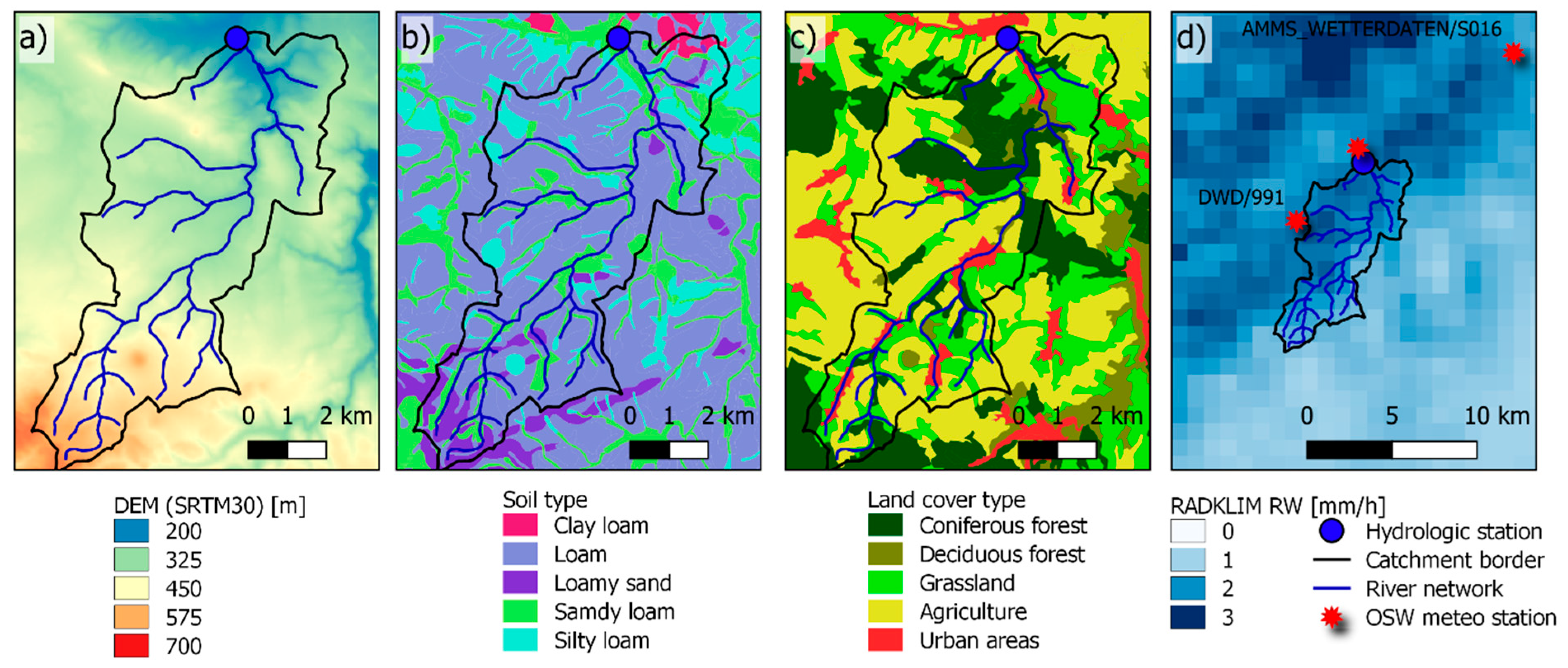
The model setup for the study was the similar to the one developed for the estimations of the water fluxes in small and medium size catchments at high spatial resolution and different soils (Luong et al. 2020). Figure 3 shows an example of the model setup for the Kreischa catchment (ID 3). A hydro response units (HRU) approach is used to estimate the water fluxes by blending maps of elevation (DEM), simplified information of land use (CORINE 2012), and soil (BK 50). The different precipitation inputs, namely the grid of RADKLIM-RW and nearby rain gauges, are illustrated in Figure 3d. Further description of the model setup can be found in Luong et al. (2020) and main land use parameters in Appendix B. In this study, the water balance simulations were conducted for ten catchments, which consist of total 50 sub-catchments and 3233 HRUs. The density of HRU for each catchment is provided in Table 1. The simulations of these HRUs with different meteorological forcing (rain gauges and radar with the consideration of wind correction) generates a large number of model runs, which requires a high computational capacity. A 17-year model run for a sub-catchment with a selected precipitation product takes about 20 min, which results in almost a week for an entire catchment and one precipitation input, even if a parallelization function is activated during the run. Thus, we decided to stick with original fixed parameterization (same for per soil and land cover type) of the framework and omit calibration process.

2.4. Wind Correction Method

As common practice, Richter’s correction (Equation (1)) was applied to rain gauge data based on the type of precipitation, mean temperature, day of the year (coefficient ε), and the information about the degree of shielding (coefficient b) (Appendix C). It can be observed that the snowier a precipitation event and the freer the shielding of the rain gauge is, the more precipitation should be compensated. In this study, the mean temperature was derived from the OSW and the shielding degree was derived from the DWD rain gauge classification [39]. According to this, more than 70% of the rain gauges in Saxony are moderately shielded; about 30% of the rain gauges have strong shielding, and only a few are free and weakly protected. We chose moderate shielding as representative for the study sites as a pragmatic solution. As a result, the same correction shielding coefficients were applied for the precipitation datasets. It should be noted that the correction was finally applied for the interpolated rain gauged precipitation and averaged precipitation for a catchment derived from RADKLIM. Instead of correcting the rain gauges before interpolation, we considered the correction only once for the interpolated rainfall for a catchment. Thus, the same procedure was implemented for the RADKLIM-RW precipitation extracted for a catchment, where the information from the rain gauges involved in the calibration was not available. Therefore, this post correction approach seems to be appropriate to avoid point-to-space transfer issue.
R K = R R + b . R R ε
RR: precipitation (mm)
RK: corrected precipitation (mm)
b, ε: coefficients of the correction function depending on precipitation type, horizon shielding, and protection of the measuring station (Table 2).
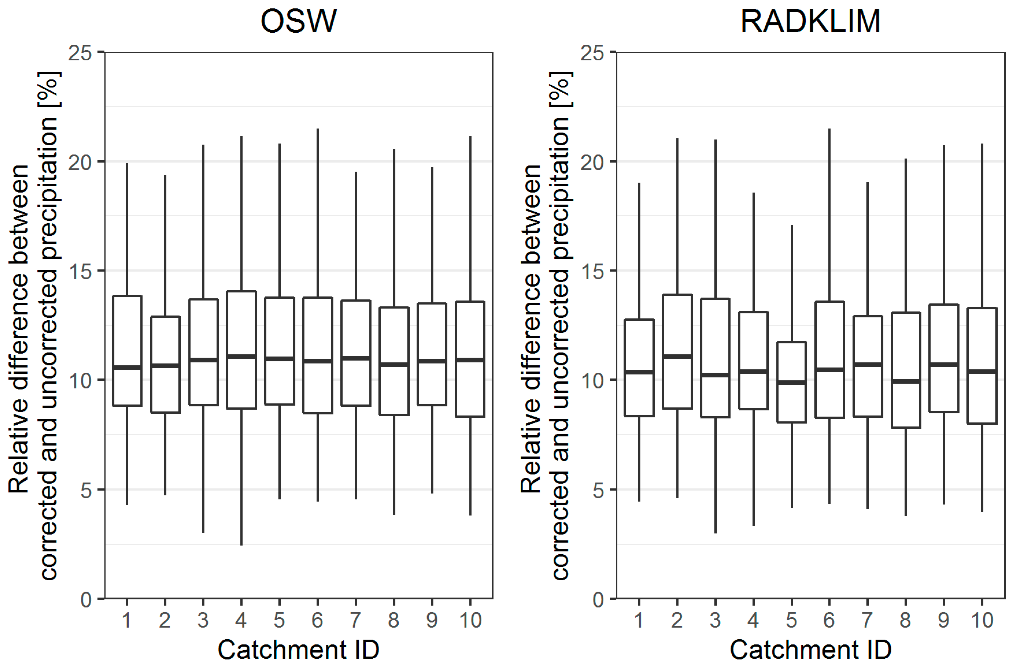
On average, approximately 10% of monthly precipitation (median values) is added for each month after applying the correction (Figure 4). The monthly variation in the relative amount of additional precipitation mainly ranges from 5% to 20%. This result is similar to the previous studies, in which the moderate degree of shielding was applied to the rain gauges in the various regions of Saxony [25,35]. Precipitation compensation is relatively stable for all catchments in both datasets (OSW and RADKLIM), as reflected in the average number of days for each precipitation event classified by the mean temperature (Table 2). During the study period, the average number of rainy days ranged from 236 to 282 and the number of days with sleet and snow were 46–59 and 38–70, respectively. An effect of topography can be observed in Tannenberg (ID), as it is the highest catchment in the study and obtained more sleet and snow days and less rainy days.

2.5. Analysis

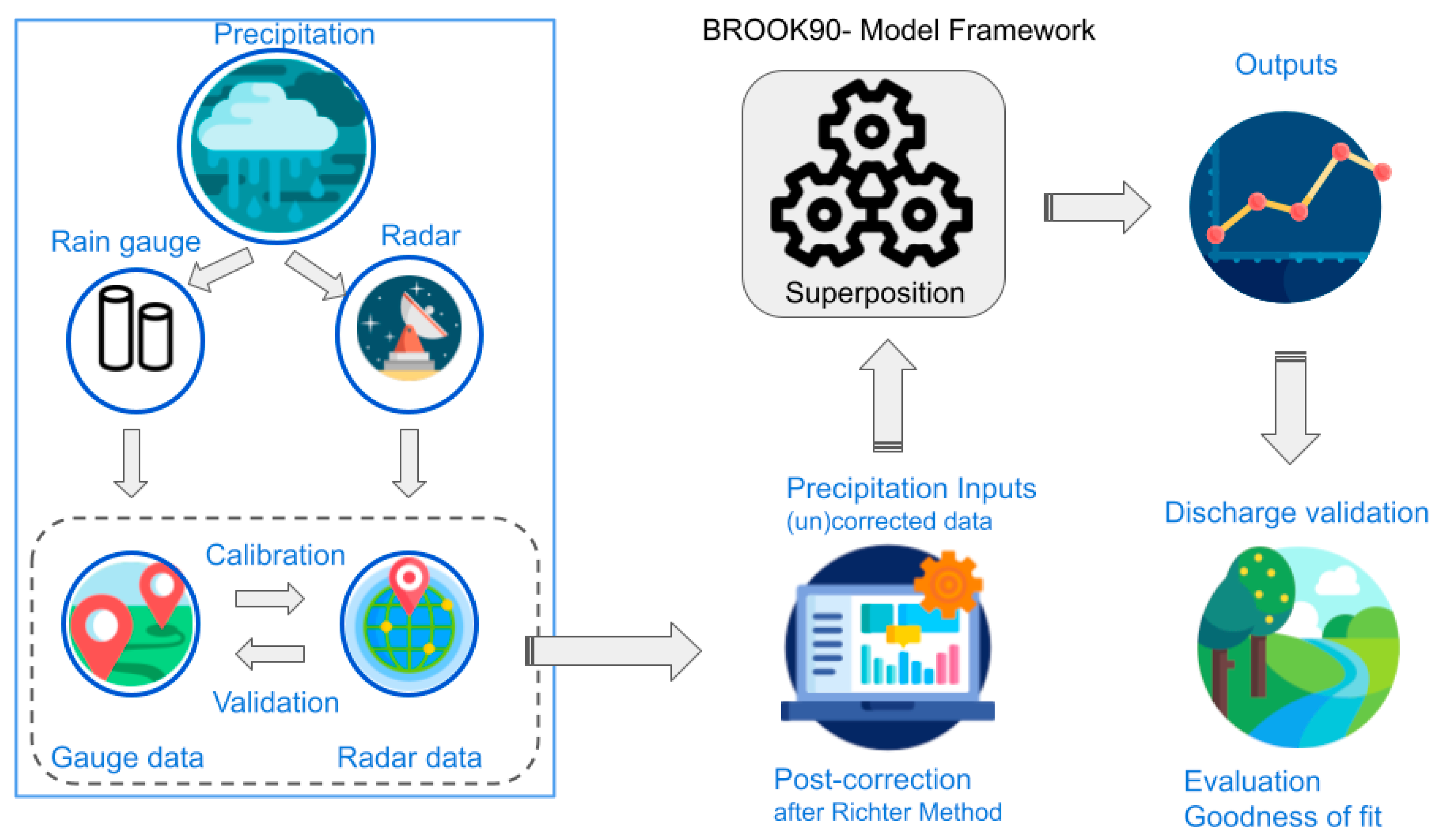
Despite the fact that both model structure and input data sources introduce uncertainty into simulated discharges, the study focuses solely on the uncertainty of the simulated water balance components due to different precipitation input, leaving parameterization schemes as well as other aspects of input data outside of the study scope. Thus, we examined the characteristics and impacts of four different precipitation datasets, namely uncorrected gauges, corrected gauges, uncorrected radar, and corrected radar. Daily, monthly, and annual precipitation sums for each catchment were compared for each of the four data sets. A statistical t-test was applied to evaluate the difference between the data sets, and the significance of the test was determined by the p values. Furthermore, we focused on the following aspects: (1) the absolute difference between precipitations derived from OSW and RADKLIM, (2) the distribution of the monthly average difference of precipitation from OSW and RADKLIM for the selected catchments, and (3) the correlation on a daily scale of precipitation in summer and winter months. The precipitation datasets were then used in the EXTRUSO framework, which output discharge values were compared to the measurements. A few goodness of fit criteria were selected to evaluate the performance of the simulations, which are described in detail below. An overview of the validation can be found in Figure 5.
Model performance was evaluated directly against observed runoff at various temporal resolutions. The simulation period was restricted to 2001–2017 (following the availability of RADKLIM-RW data). Additionally, we excluded the three-month spin up period at the start of each BROOK90 model run to allow soil moisture to reach a stable state in water balance processes.
As common in hydrological research and other disciplines [38,40], the Kling–Gupta efficiency (KGE) [41] and its decomposition into three components (correlation, mean bias, and variability bias) were chosen to quantify the model outputs (Equation (2)).
K G E = 1 R 1 2 + α 1 2 + β 1 2
where R is the correlation coefficient, α = σsim/σobs is the ratio of the standard deviations σ of simulations and observations, and β = μsim/μobs is the ratio of the simulated and observed means μ. KGE equals 1 for a perfect fit of the simulation when R, α, and β are all at their optimal value 1. One of the advantages of using KGE is the consideration of multiple aspects in the comparison. According to Knoben et al. (2019) [42], the KGE value at −0.41 shows that the model performance is as good as the observed mean flow. Our goal was to compared simulations of the BROOK90 water balance model with observed discharges to evaluate performance accuracy for ten catchments with three temporal aggregations, namely daily, monthly, and annual. In addition, empirical quantiles of the 90th, 50th, 10th, and 1st percentiles were applied to derive low, medium, high, and extreme discharge values, respectively.

3. Results

3.1. Comparing Precipitation Datasets

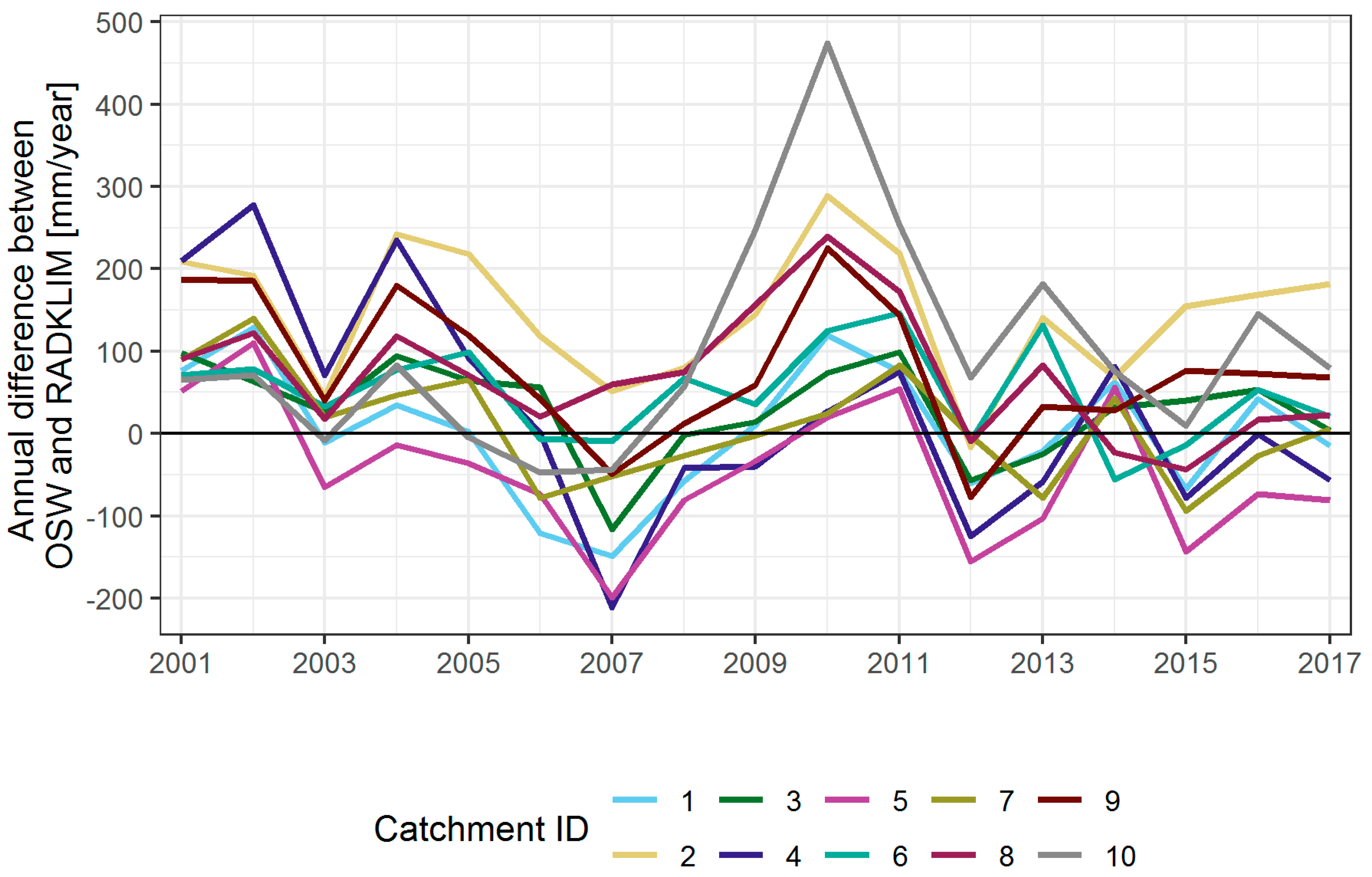
The annual precipitation products derived from OSW and RADKLIM data without the correction for the ten catchments were compared over the 2001–2017 period. Figure 6 shows generally no clear pattern in differences between the two datasets for the selected catchments. Precipitation from gauges can be higher or lower than precipitation from radar and varies from year to year and from catchment to catchment. It can be noted that the deviation was lower for the dry years (e.g., 2003, 2014) compared to the wet years (e.g., 2010), which is probably a result of the small number of selected catchments or uncertainties in precipitation in the datasets obtained from radar beams and extreme events [16,17]. The absolute difference ranges between 100 and 200 mm. Previous studies showed that the QPE radar precipitation show underestimations compared to precipitation from rain gauges [17,25], particularly in mountainous regions where radar beams are often blocked by orography. This effect can be clearly observed in the Tannenberg catchment (ID 10, 662 m.a.s.l.) in 2010, which is considered as a “wet year” with large precipitation sums. Here, the difference between gauges and radar reached the maximum values of over 400 mm on an annual scale. Moreover, the positive bias for the median values of the ten catchments (Table 3) was statistically significant at a daily scale, suggesting that precipitation from gauges is generally higher than from radar. This finding was also confirmed by the study of Kreklow et al. (2019), in which different precipitation datasets were compared in high resolution for the entire Germany. However, precipitation sums from radar were found higher than gauges at the catchment 1, 4, and 5 on a monthly scale and at the catchment 5 on an annual scale. This negative bias was, nevertheless, statistically insignificant (Table 3). Thus, it suggests that the difference of the two precipitation datasets can be arbitrary.
Examining the difference between the two precipitation datasets on different temporal scales revealed a clearer clustering of the discrepancy in the catchments. Two periods, namely winter (October–March) and summer (April–September), showed different characteristics of how the differences are allocated among the study sites (Figure 7). While gauge precipitation in the summer months was mostly higher than radar precipitation, ranging 0–20 mm, with maximum values found in July, the differences in the winter months are divided into two groups associated with the location of the selected catchments. One group (Group 1), where gauge precipitation was found higher than the precipitation from radar resulting an overall higher annual precipitation (Figure 6), includes Holtendorf, Niedermuelsen, Niederzwoenitz, Reicherbach-Oberlausitz, and Tannenberg (IDs 2, 6, 8, 9, and 10, respectively). The other group (Group 2), where RADKLIM indicated higher precipitation in the winter months, includes Grossschweidnitz, Kreischa, Krummenhennersdorf, and Neustadt (IDs 1, 3, 4, and 5, respectively). This can be explained by the distances between the catchments and radar station (Dresden, Klotzsche in our study). Pöschmann et al. (2020) and Winterrath et al. (2018) have showed that the further a study site is from the location of a radar station, the lesser precipitation is captured. This can be observed in Group 1, where distances of the catchments to the radar station in Dresden are longer than the ones in Group 2 (refer to Figure 1).
Furthermore, the radar precipitation was found to be higher than gauge-derived one only in the winter months, particularly in December and January, while the ground stations record more precipitation overall than radar system in the summer months. Thus, in this section, we further examined the correlation of daily precipitation between the two datasets at the study sites. Figure 8 generally shows a high correlation of daily precipitation from OSW and RADKLIM data in all selected catchments (R > 0.8, despite of the Holtendorf catchment in summer). This has assured the similar distribution of the precipitation datasets. The correlations in winter (from October to March), when snow and sleet can possess a substantial part in total precipitation amounts, were found even higher than in summer (from April to September). This could be associated with convective rainfall events, which often occur in summer in the study areas. Due to the very local appearance of such events, ground stations with their limited density could not adequately capture their intensity as shown in the study of Kreklow et al. (2019). On the other hand, radar images have the advantage of providing adequate spatial coverage for such events, so there discrepancies in comparing precipitation amounts from ground stations and radar-based method are quite a common case [2,14,43]. This step also tested the quality of precipitation from RADKLIM product before it was used in the water balance simulations.

3.2. Impact to Water Balance Processes

3.2.1. Water Balance Components

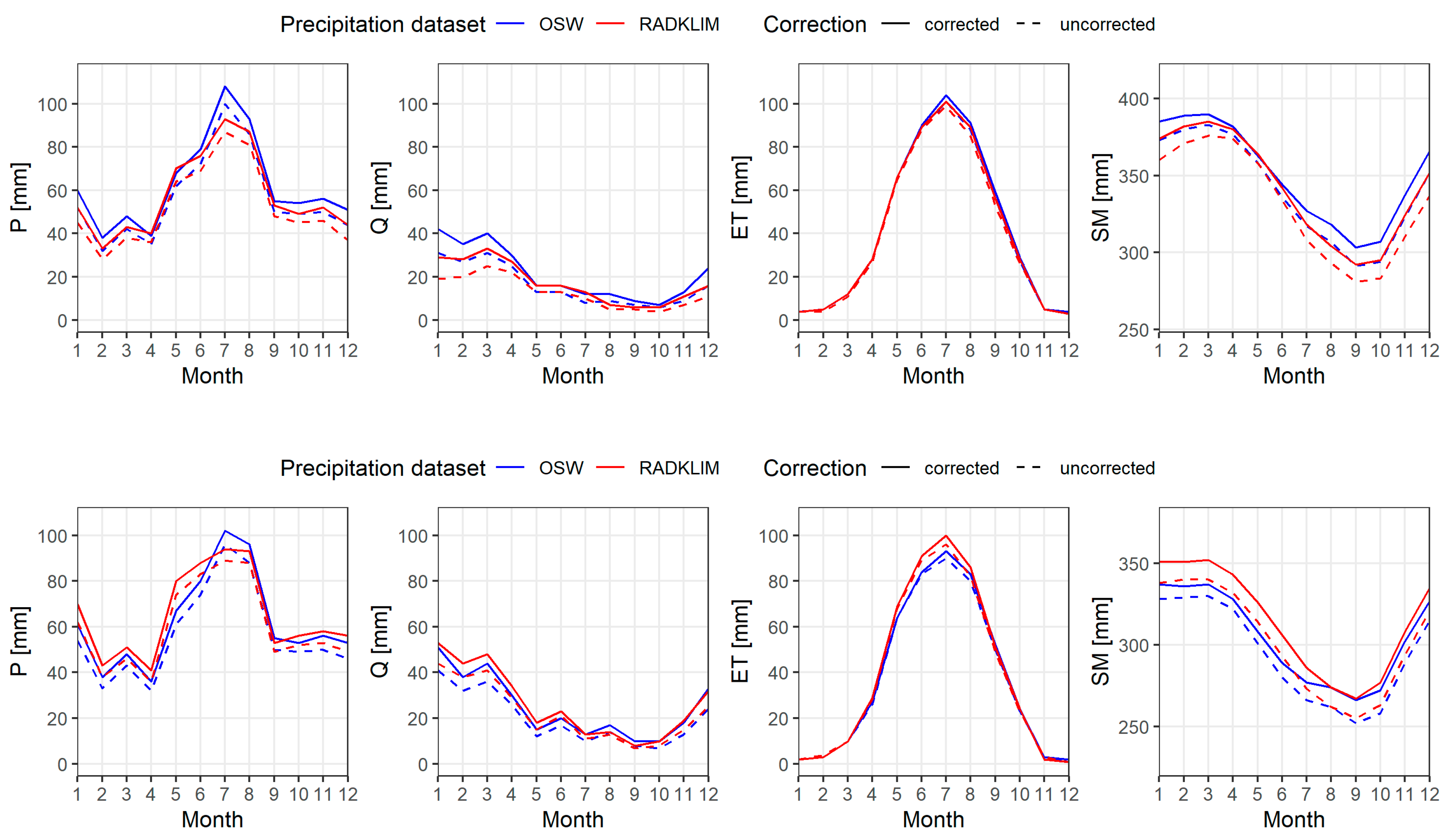
The difference between the two precipitation products, in particular their distribution during the year, leads to different impacts to simulated water balance components. Figure 9 shows two examples with the contrast that in one case the precipitation from rain gauges is larger than the precipitation from the radar (Holtendorf catchment) and in another case vice versa (Niederoderwitz). The model outputs with uncorrected precipitation serve as an uncertainty range when the correction process is not considered. In general, the higher precipitation amount, the more discharge, evapotranspiration, and soil moisture is generated. However, this is more evident for discharge (winter months) and soil moisture (summer months) than for evapotranspiration. This can be explained by the limitation of energy input despite the availability of water in the sites and saturated soil in the winter. As shown in the previous section, rain gauges tend to record more precipitation (10–20 mm monthly average) in the summer months (June–August) than radar, which has a greater impact on ET and soil moisture than discharge. Climatologically, low discharge is typical in the study sites due to the high rate of evapotranspiration and large soil retention capacity. Thus, the difference in precipitation between the two products is reflected in the change in soil moisture and ET if energy input is present. A quantitative assessment, however, can be made only for discharge (see in next sections) due to the availability of measurements. The limitations of soil moisture and ET measurements at the catchment scale leave the comparison at the visual level and physical plausibility.

3.2.2. Discharge Simulation

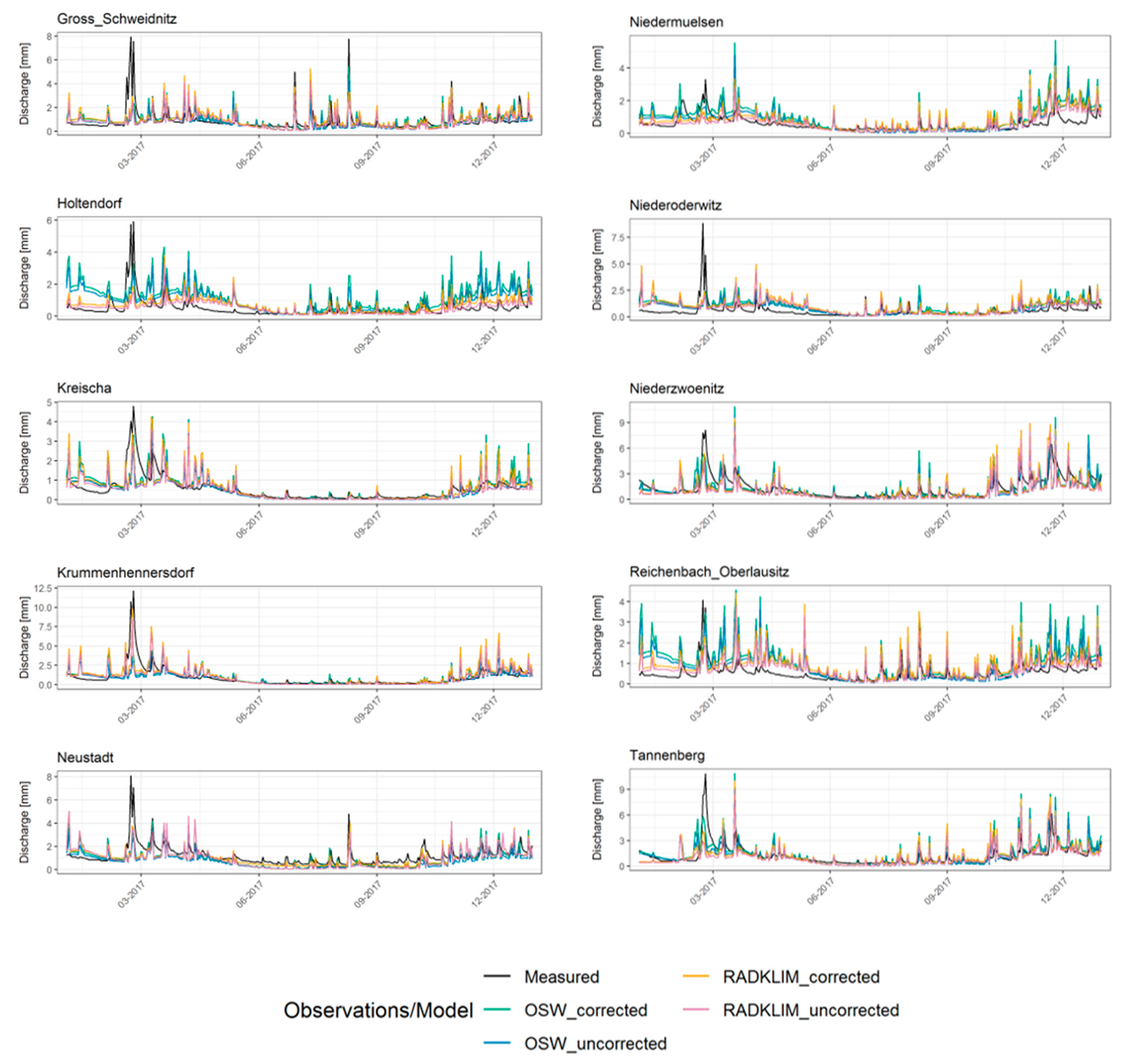
Precipitation is the only model input variable that differs between the simulation scenarios in this study, and it was noted that no calibration process was used in fitting the model parameters to preserve their physical meaning. Although we acknowledge that there are many sources of uncertainty in catchment modeling, this framework was developed to separate the effects of using radar and gauge precipitation and their corrected values as model data with respect to runoff simulation accuracy. A visual comparison of the gauge and radar simulated discharges on a daily scale (exemplary for 2017) shows that the BROOK90 simulations are in approximate agreement with the observed discharge (Figure 10). While the flood peaks are well captured, the model performance resulted in poor performance for some low flow periods particularly in the Holtendorf and Neustadt catchments (ID 2 and 5, respectively). This is not only related to the non-calibration approach, but also the location of the catchment at the border with Czech Republic and Poland, where the number of meteorological stations is limited (Figure 2). This resulted in the largest discrepancy between the two datasets for the catchments (previous section). Particularly, there appears to be a systematical overestimation of the discharge for both datasets in the Holtendorf catchment (ID 2). With that noted, RADKLIM data produced a better performance here than OWS data in this catchment (Figure 10). Although the basic water budget volumes are realistic for systems in the study sites with both data sets, the rain gauged simulations show higher discharges than the simulations with radar. The simulations with corrected precipitation resulted higher discharges in both data sets, but by no mean lead to a systematically better model performance.

3.2.3. Skill Scores Evaluation

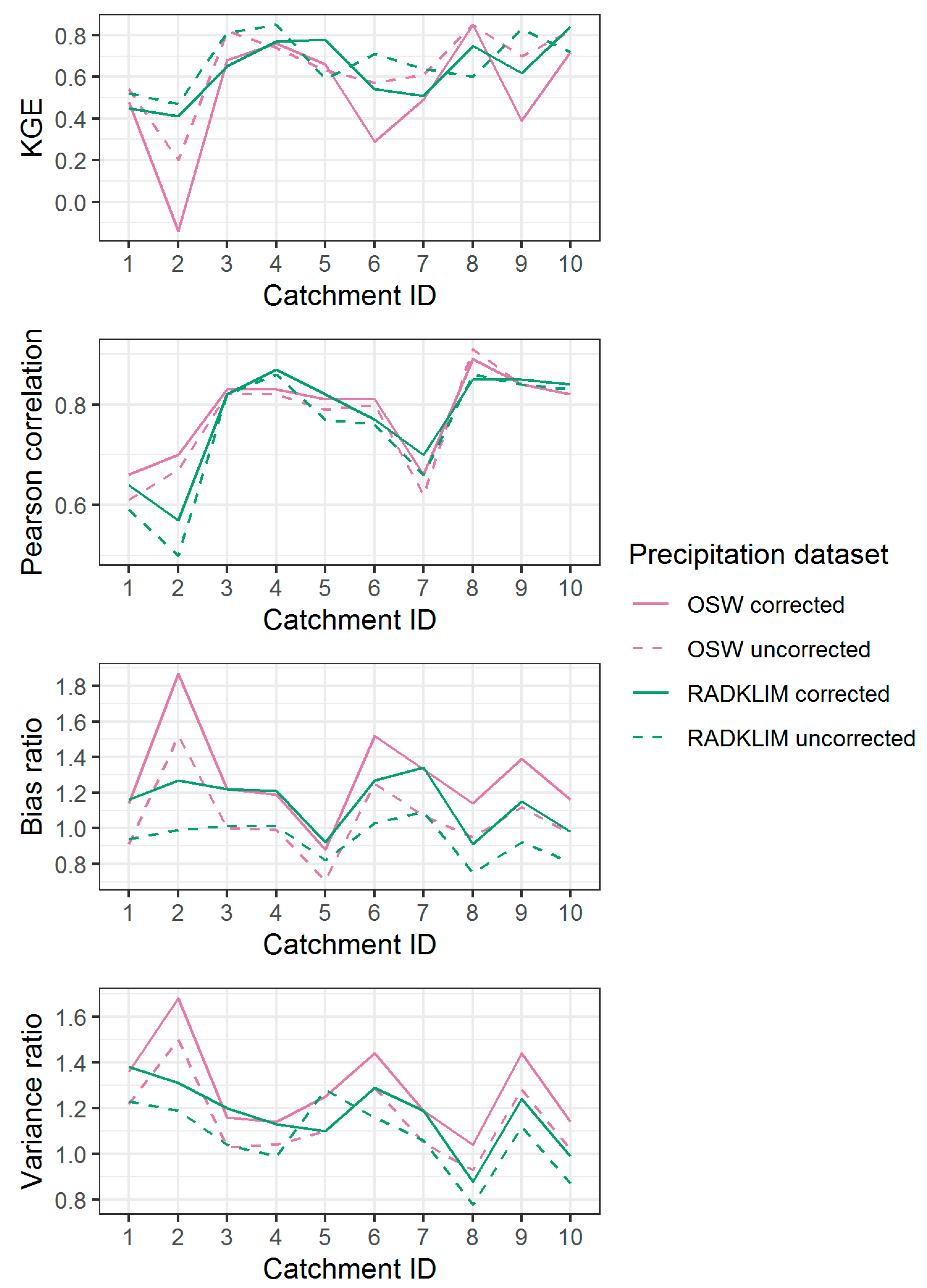
The sensitivity of a model prediction strongly depends on the characteristics of a catchment such as size or/and orography, land use, and meteorological input [10]. Therefore, we examined the performance of the model with different precipitation data sets for each selected catchment based on the selected skill scores, which vary among the catchments (Figure 11). With the exception of the Holtendorf catchment, KGE values ranged from 0.20 to 0.63 on the daily scale (not shown in Figure) and from 0.41 to 0.85 on the monthly scale for the model performance with four sets of precipitation inputs. Similar to previous studies [37,38], the high variability of daily discharge was reduced by averaging over a longer period (monthly), which resulted in a better agreement between observed and simulated discharge. The best performance was found for Kreischa (ID 3), Krummenhennensdorf (ID 4), and Niederzwoenitz (ID 8) catchments (KGE > 0.7) for both datasets. On the other hand, a relatively lower skill score (KGE < 0.5) was observed in Grossschweidnitz, Holtendorf, Niedermuelsen, and Reichenbach Oberlausitz (ID 1, 2, 6, and 9, respectively), due to a relatively big bias and overestimation of variance ratio. Nevertheless, according to [42], the model outputs in the selected catchments are reliable and comparable with similar studies [37,38,44].
The primary advantage of the KGE criteria is the ability to obtain a deeper understanding of model uncertainty through its decomposition. A closer look at the KGE components (Figure 10) shows that correlation coefficients for the catchments are high (r > 0.8), with the exception of the catchment IDs 1, 2, and 7, and the main problems were found in overestimations of the mean (bias ratio > 1 and variance ratio > 1) (except for simulations with radar at the catchments 8 and 10). Overall, we found that neither RADKLIM nor OSW data performs better than the other. While the model with RADKLIM data performed better in Holtendorf, Neustat, Niedermuelsen, Reichenbach Oberlausitz, and Tannenberg (IDs 2, 5, 6, 9, and 10, respectively), the model with gauge precipitation performed better in Großschweidnitz, Kreischa, and Niederzwoenitz (IDs 1, 3, and 8, respectively). However, an interesting result can be seen at the Tannenberg catchment, where the quality of the radar-derived precipitation was found to be poor due to beam blockages [25], yet still resulted in reliable performance (KGE > 0.7).
In addition, the effect of Richter correction of precipitation data sets on model performance reveals surprising results. Most catchments show no model improvement with the inclusion of corrected data. Only three catchments (IDs 5, 8, and 10) indicated better performances with the additional precipitation input for both data sets. This can be explained by their locations. Catchment 5, 8, and 10 are located in the Ore Mountains with an elevation of 386, 600, and 662 m.a.s.l, respectively, where an underestimation endured by wind in measurements often occurs [16,45]. In addition, the most sleet and snow days were also observed in these three catchments (Table 2). Hence, the Richter correction resulted in a positive effect at these study sites. Although, the correction helped to improve the correlation coefficients in most of the catchments, it resulted in high bias (>1) and variances (>1). Thus, here, discharge validation generally failed to show a significant improvement of the runoff simulations. The opposite, however, was true for low elevation areas. Skill scores declined with compensated precipitation.
Besides the main drawbacks of the model framework and parameters, it is worth mentioning the influences of meteorological measurements, especially their spatial distribution within the study catchments. The low performances for the catchment 2, 7, and 9 can be generally associated with the poor coverage by precipitation gauges in these locations, where the density of gauges is lower than for the other catchments (Figure 2). Moreover, the skill scores for radar data here were better than those for gauge precipitation. Figure 2 shows that the maximum values of distances for the precipitation stations are even larger than their areas (Table 1), which can make the information about the spatial variability of precipitation events misleading. Thus, we advise to use radar for catchments that contain few precipitation gauges within their boundaries. Other studies also confirmed a similar dependence on gauge coverage when comparing radar- and gauge derived runoff simulations [4,14,46]. It should be noticed that a better coverage of stations in the hydrometeorological automated data system for small catchments may lead to different results. Further research is needed to determine the spatial and temporal thresholds for the required coverage by gauges, under which modelers should rely on radar precipitation [20,47].

3.2.4. Discharge Magnitude Comparision

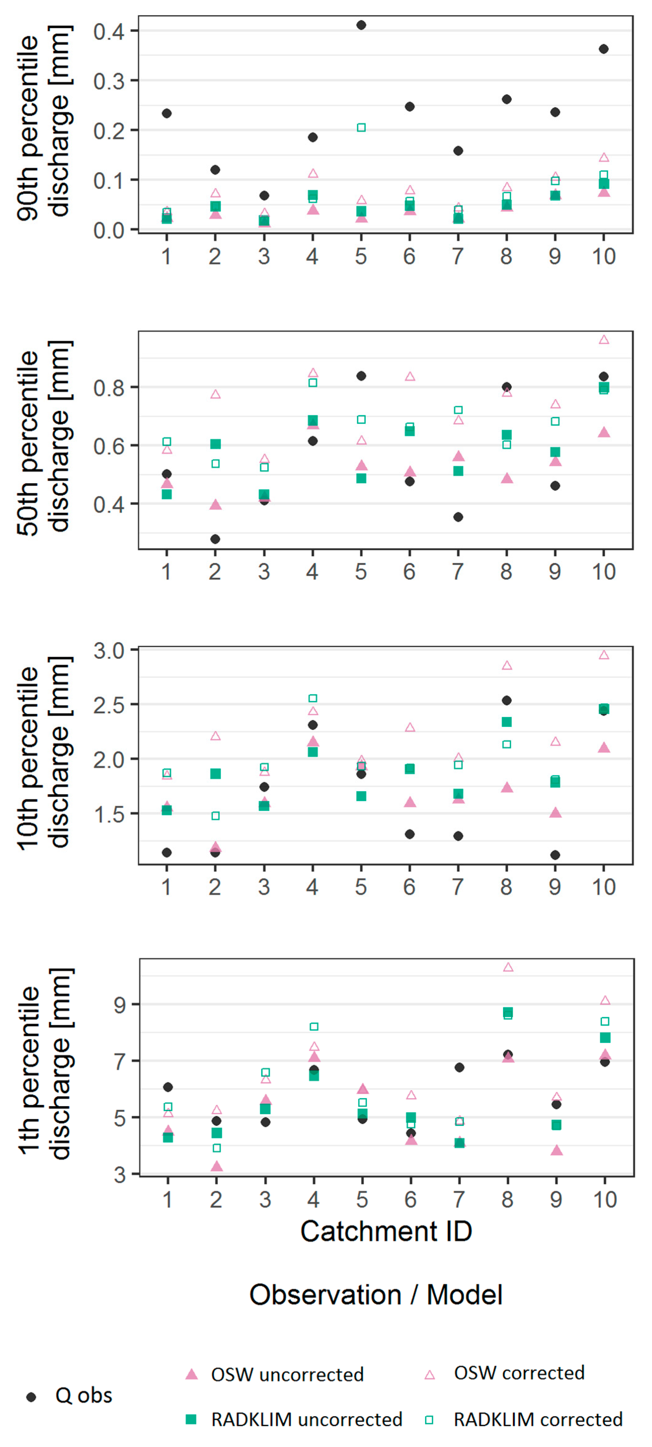
Simulated low discharges (90th percentile), medium discharge (50th percentile), high discharge (10th percentile), and extreme discharge (1st percentile) were compared to observations for each precipitation input and catchment (Figure 12). The framework with gauge precipitation tended to underestimate low flow. The radar simulations produced even lower low discharges but demonstrated improvement over the gauge data in simulating extreme flows. Comparison of the medium and high flows showed a slow shift towards general overestimation by the model. These discharge results demonstrated that precipitation plays a minor role compared to model setup (parameterization) in simulating low flows, while it becomes more important for higher flows. The Richter correction contributed a positive effect at low flows but rather insignificant. Moreover, no clear improvement due to correction was observed at other flow magnitudes. Assuming that observed discharges are accurate, gauge precipitation appeared to advance estimations of low flows; whereas radar, which typically underestimates light precipitation, performed better for heavier precipitation events.

4. Discussion

The results can be associated with the drawbacks of the BROOK90 model and the framework itself, even though this model has a good physically-based description of the evaporation process. The model uses a two-layer version of Penman–Monteith equation, namely Shuttleworth and Wallace to estimate potential evapotranspiration separately for canopy and soil surface accounting for surface energy budget and gradient for the sensible heat flux, respectively. However, canopy parameters are assumed as constants, so phenology or tree growth is neglected, which can lead to underestimation of evapotranspiration, in particular in agriculture sites during the vegetation period. Moreover, the model includes an upper limit for potential evapotranspiration, which may be exceeded. Hence, evapotranspiration can be constrained by the energy input despite of the availability of water supply. Last but not least, one of the major factors for the overestimation of the framework is the lack of information of ground water process, which greatly limits the parameterization, leading to higher uncertainties at lower altitudes.
Our results contribute to the understanding of the complex relationships between model structure, precipitation data resolution and accuracy, and importance of spatial and temporal scaling considerations in catchment modelling [2,48,49]. Several researchers also suggest that the application of the Richter correction to a certain precipitation product in hydrological simulations must be carefully addressed. First, the modelling community requires a thorough investigation of the role of model structure in exploiting information on spatial distributions of precipitation. In semi distributed models and lumped models, the spatial aggregation can eliminate any information provided by high-resolution data, making the increased processing demands unnecessary. The relationship between model structure and input data resolution needs to be explicitly studied [50,51]. Second, model users typically have some control over the spatial discretization level. For example, in lumped models, the user can choose between [37] or regular grids for HRU subset [38]. This decision is based on modelling objectives but could be particularly important in the context of this discussion because spatial variability in precipitation can only be accounted for on the HRU level. If modelers choose to consider the heterogeneity of a catchment in terms of streamflow response, the computational time may be much longer, which can limit the calibration options (as, i.e., in our study). Thus, addressing a study of how much accuracy will be improved by varying levels of discretization for different model configurations would be a great contribution for the modelling community (i.e., [50,52]). Thirdly, it is very reasonable to expect that there will be differences in the accuracy of precipitation data (from all sources) when different types of storm structures and precipitation types are considered. Besides the DWD meteorological network, other available open data sources, which can be integrated in the OSW, should be considered and enhanced to increase sensors’ density. Finally, a study to analyze different precipitation interpolation schemes at different time scales in relation to the available data in different networks in order to improve the accuracy of discharge simulations should provide helpful information for the modelers [53,54].

5. Conclusions

In this study, we presented an application of radar-derived precipitation (RADKLIM RW), meteorological variables from OSW in a water balance model, as well as the effects of wind corrections. RADKLIM data were extracted for the ten selected catchments and compared with interpolated rainfall from rain gauges integrated with an OSW. In general, rain gauge-derived precipitation was slightly higher than that extracted from radar, which has been confirmed in previous studies [16,17,20]. However, both data sets delivered an acceptable performance with regards to water balance simulations. Furthermore, there is no clear trend in the difference between the two data sets, with the exception of the winter months (October to March) when a larger discrepancy between the two data sets was observed in the catchments that are closer to the radar station. The correlation between the two data sets was more pronounced in summer than in winter due to convective events. The results of this study indicate that there is currently no generally preferable precipitation product for water balance modelling. The decision of whether to use radar, gauge, or other precipitation data should be predicated on the basis of desired spatial and temporal scales. One should also take into account the availability of computing resources to use higher resolution products, i.e., high-quality gauge data within or near the catchment versus the complexity of handling gridded precipitation data (as contrasted with the simpler point-based time series of gauge data). Model structure and/or its configuration also plays a crucial role. Here, we used a pseudo-semi distributed model and run it at a relatively fine level of HRUs derived from high-resolution land use and soil maps. However, the implications of the choice for precipitation data go beyond discharge modeling, as several sources of bias are involved.
The study also revealed that applying a wind correction for precipitation such as the Richter method increased monthly precipitation by approximately 10%, and that orography has an effect on the classification of precipitation by temperature. However, even such a simple compensation such as the Richter method to conventional precipitation should be used with caution. This is because it would most likely result in a substantial increase runoff, leading to larger biases and variances compared to measurements. Our results suggest that application of the wind correction method could be more appropriate in higher elevation catchments, while catchments at low elevation would result in lower performance to the correction. Nevertheless, there is considerable potential to improve model results. The accuracy of the spatial interpolation of the meteorological variables can be refined by incorporating additional monitoring networks. By employing dynamic land use, deforestation, storm degradation, the habitat growth of a young forest, and the seasonal variation of the LAI can be also addressed. Additionally, providing local cognition of meteorological and plant properties can ameliorate the model performances. This study should be extended to other catchments in other German states to more thoroughly test the RADKLIM data within Germany and its application in water balance modeling.

Author Contributions

Conceptualization T.T.L. and C.B.; methodology T.T.L., I.V. and R.K.; software T.T.L. and R.K.; results T.T.L., I.V. and J.P.; writing: original draft preparation T.T.L., J.P. and I.V.; review C.B., D.G., J.P. and R.K., editing T.T.L., I.V. and D.G.; visualization T.T.L. and I.V.; supervision C.B. All authors have read and agreed to the published version of the manuscript.

Funding

The research was supported by the EXTRUSO project funded by the European Social Fund (ESF) under award no. 100270097 and the Erasmus Mundus GroundwatCH educational program, as well as by open access funding from the TU Dresden Publication Fund.

Institutional Review Board Statement

Not applicable.

Informed Consent Statement

Not applicable.

Data Availability Statement

All data used in the study are available and can be provided upon request (about 25 GB). The model framework is packaged as an xtruso package and available on Github (https://github.com/GeoinformationSystems/xtruso_R (accessed on 10 March 2020)). The runoff data were collected from the local open platform and the gauge and radar precipitation data are provided by the DWD. An illustration of how the model works and how the results are analyzed is available in the Zenodo Data Store (https://doi.org/10.5281/zenodo.5727126 (accessed on 10 March 2020)).

Acknowledgments

We thank all colleagues (Philipp Körner, Majana Heidenreich and Gesa Bedbur) at the Chair of Meteorology in Tharandt for their support. A special thanks to Stefan Wiemann for creating the xtruso package. We are also grateful for the comments and materials of Tanja Winterrath regarding the RADKLIM product.

Conflicts of Interest

The authors declare no conflict of interest.

Appendix A

The RADKLIM dataset was processed and integrated in the “xtruso” package (https://github.com/GeoinformationSystems/xtruso_R (accessed on 10 March 2020)). The following workflow describes the derivation from the raw data from the DWD to data input for a catchment.
Step1: RADKLIM raw data processing
RADKLIM- RW binary file from the specified link following the official DWD file pattern is used to read the data, after the product configuration is set. In this process, flagged pixels are removed from the RADKLIM image and set to the value NA. After parsing the binary file, we obtain the data as a raster object. The coordinates in the RADKLIM coordinate reference system are derived from column-row-index or cell number, from which we can obtain indices and weights over the RADKLIM raster for a given polygon. A bounding box is also considered in this step.
Step 2: Create NetCDF file for RADKLIM images
The structure of the NetCDF is based on the horizontal and vertical dimensions of the RADKLIM extent. The time dimension is set as unlimited and the attributes as default values. The NetCDF files are created from RADKLIM data based on the abovementioned setting, sorted by year, and stored in a separate folder. As a result, the NetCDF files contain the parameters such as configuration, timestamp, and year, which allows extracting the data in a period of interest using the index associated with the timestamp.
Step 3: Read time series from RADKLIM NetCDF file for a catchment
The parameters required to read time series for a catchment from the created NetCDF files are start date, end date, time format, time zone, an extent or a polygon for which statistics are calculated, statistics flag to request a specified statistic for an extent, and projection if extent is specified as a json string. When the information is provided, we can obtain a final data frame that calculates the mean values for each time stamp (hourly in this case) for the desired period within the extent. Since the model requires daily data input, the extracted time series are aggregated from hourly to daily.
Step 4: Apply correction factor
Similarly to the precipitation from rain gauges, the precipitation from RADKLIM-RW is applied in two versions: uncorrected and corrected. The details of the Richter correction can be found in the following section.

Appendix B

Table A1. Physical meanings and values of main parameters of the BROOK90 model for different vegetation at the study sites.
Parameters
Abbreviation
Physical MeaningConiferous ForestDeciduous ForestAgricultureGrass
RELHTpairs of day of the year and relative height between 0 and 111(1,0,100,0,
213,1,278,1,
308,0,366,0)
(1,0.1,115,0.1,
145,1,268,1,
298,1,366,0.1)
RELLAIpairs of day of the year and relative LAI between 0 and 1(1,0.8,60,0.8,
90,0.8,120,1,274,
0.9,305,0.8,366,0.8)
(1,0,54,0,84,1,
299,1,329,0,366,0)
(1,0,100,0,
213,1,278,1,
308,0,366,0)
(1,0,115,0,
145,1,268,1,
298,0,366,0)
ALBalbedo or surface reflectivity without snow0.070.180.220.2
ALBSNalbedo or surface reflectivity with snow0.30.230.50.5
KSNVPhydraulic conductivity at field capacity corresponding to THETAF and PSIF for a soil layer0.30.311
Z0Gground surface roughness (m)0.020.0030.0050.03
MAXHTmaximum canopy height for the year29262.20.8
MAXLAImaximum projected LAI for the year7.5644
MXRTLNmaximum length of fine roots per unit ground area (m2/m2)310032001101000
MXKPLmaximum plant conductivity (mm/day MPa)8888
FXYLEMfraction of plant resistance that is in the xylem0.50.500
CSratio of projected SAI to HEIGHT0.0350.45-0.035
GLMAXmaximum leaf conductance (cm/s)0.350.11.31.5
LWIDTHaverage leaf width (m)0.0040.10.10.01
CRextinction coefficient for photosynthetically active radiation in the canopy0.50.60.70.7

Appendix C

Table A2. The dependency of coefficients of the correction function (b and ε in Equation (1)) on precipitation type and shielding degree, Richter (1995). Remark: the classification of precipitation types based on temperature is only valid for Germany.
Precipitation Type Tmean (TM)
(Valid for Germany)
εShielding Degree (b)
FreeWeakModerateStrong
Rain (summer)TM > 3.0 °C0.380.3450.3100.2800.245
Rain (winter)0.460.3400.2800.2400.190
Mixed precipitation
(sleet)
3.0 °C ≤ TM ≤ −0.7 °C0.550.5350.3900.3050.185
SnowTM < −0.7 °C0.820.7200.5100.3300.210

References

  1. Beven, K. Towards an alternative blueprint for a physically based digitally simulated hydrologic response modelling system. Hydrological Processes. 2002, 206, 189–206. [Google Scholar] [CrossRef] [Green Version]
  2. Borga, M.; Esposti, S.D.; Norbiato, D. Influence of errors in radar rainfall estimates on hydrological modeling prediction uncertainty. Water Resources Research. 2006, 42, 1–14. [Google Scholar] [CrossRef] [Green Version]
  3. Rozalis, S.; Morin, E.; Yair, Y.; Price, C. Flash flood prediction using an uncalibrated hydrological model and radar rainfall data in a Mediterranean watershed under changing hydrological conditions. J. Hydrol. 2010, 394, 245–255. [Google Scholar] [CrossRef]
  4. Zoccatelli, D.; Marra, F.; Armon, M.; Rinat, Y.; Smith, J.A.; Morin, E. Contrasting rainfall-runoff characteristics of floods in Desert and Mediterranean basins. Hydrol. Earth Syst. Sci. Discuss. 2018. [Google Scholar] [CrossRef] [Green Version]
  5. Tarolli, P.; Borga, M.; Morin, E.; Delrieu, G. Analysis of flash flood regimes in the North-Western and South-Eastern Mediterranean regions. Nat. Hazards Earth Syst. Sci. 2012, 12, 1255–1265. [Google Scholar] [CrossRef] [Green Version]
  6. Braud, I.; Roux, H.; Anquetin, S.; Maubourguet, M.M.; Manus, C.; Viallet, P.; Dartus, D. The use of distributed hydrological models for the Gard 2002 flash flood event: Analysis of associated hydrological processes. J. Hydrol. 2010, 394, 162–181. [Google Scholar] [CrossRef] [Green Version]
  7. Blöschl, G.; Reszler, C.; Komma, J. A spatially distributed flash flood forecasting model. Environ. Model. Softw. 2008, 23, 464–478. [Google Scholar] [CrossRef]
  8. Corral, C.; Velasco, D.; Forcadell, D.; Sempere-Torres, D.; Velasco, E. Advances in radar-based flood warning systems. The EHIMI system and the experience in the Besòs flash-flood pilot basin. In Flood Risk Management: Research and Practice; CRC Press: Boca Raton, FL, USA, 2009; Volume 332, pp. 1295–1303. [Google Scholar]
  9. Kirstetter, P.E.; Delrieu, G.; Boudevillain, B.; Obled, C. Toward an error model for radar quantitative precipitation estimation in the Cévennes-Vivarais region, France. J. Hydrol. 2010, 394, 28–41. [Google Scholar] [CrossRef]
  10. He, X.; Vejen, F. An Opera θ onal Weather Radar—Based Quan θ ta θ ve Precipita θ on Es θ ma θ on and its Applica θ on in Catchment. Water Resour. Model. 2011, 10, 8–24. [Google Scholar]
  11. Borga, M.; Tonelli, F.; Moore, R.J.; Andrieu, H. Long-term assessment of bias adjustment in radar rainfall estimation. Water Resour. Res. 2002, 38, 8-1–8-10. [Google Scholar] [CrossRef] [Green Version]
  12. Knöll, P.; Zirlewagen, J.; Scheytt, T. Using radar-based quantitative precipitation data with coupled soil- and groundwater balance models for stream flow simulation in a karst area. J. Hydrol. 2020, 586, 124884. [Google Scholar] [CrossRef]
  13. Villarini, G.; Krajewski, W.F.; Ntelekos, A.A.; Georgakakos, K.P.; Smith, J.A. Towards probabilistic forecasting of flash floods: The combined effects of uncertainty in radar-rainfall and flash flood guidance. J. Hydrol. 2010, 394, 275–284. [Google Scholar] [CrossRef]
  14. Meissner, D.; Gebauer, S.; Schumann, H.A.; Pahlow, M.; Rademacher, S. Analysis of radar-based precipitation products as input data to improve water-level forecasting for navigation on the Rive Rhine. Hydrol. Wasserbewirtsch. 2012, 56, 16–28. [Google Scholar]
  15. Winterrath, T.; Rosenow, W.; Weigl, E. On the DWD quantitative precipitation analysis and nowcasting system for real-time application in German flood risk management. IAHS- Publ. 2012, 351, 323–329. [Google Scholar]
  16. Kronenberg, R.; Bernhofer, C. A method to adapt radar-derived precipitation fields for climatological applications. Meteorol. Appl. 2015, 22, 636–649. [Google Scholar] [CrossRef]
  17. Kreklow, J.; Tetzla, B.; Kuhnt, G.; Burkhard, B. A Rainfall Data Intercomparison Dataset of RADKLIM, RADOLAN, and Rain Gauge Data for Germany. Data 2019, 4, 118. [Google Scholar] [CrossRef] [Green Version]
  18. Winterrath, T.; Brendel, C.; Hafer, M.; Junghänel, T.; Klameth, A.; Lengfeld, K.; Walawender, E.; Weigl, E.; Becker, A. Radar Climatology (RADKLIM) Version 2017.002 (RW), Gridded Precipitation Data for Germany. 2017. Available online: https://opendata.dwd.de/climate_environment/CDC/grids_germany/hourly/radolan/reproc/2017_002/bin/ (accessed on 10 January 2020).
  19. Lengfeld, K.; Winterrath, T.; Junghänel, T.; Hafer, M. Characteristic spatial extent of hourly and daily precipitation events in Germany derived from 16 years of radar data. Meteorol. Z. 2019, 28, 363–378. [Google Scholar] [CrossRef]
  20. Stisen, S.; Højberg, A.L.; Troldborg, L.; Refsgaard, J.C.; Christensen, B.S.B.; Olsen, M.; Henriksen, H.J. On the importance of appropriate precipitation gauge catch correction for hydrological modelling at mid to high latitudes. Hydrol. Earth Syst. Sci. 2012, 16, 4157–4176. [Google Scholar] [CrossRef] [Green Version]
  21. Stisen, S.; Sonnenborg, T.O.; Hojberg, A.L.; Troldborg, L.; Refsgaard, J.C. Evaluation of Climate Input Biases and Water Balance Issues Using a Coupled Surface—Subsurface Model. Vadose Zone J. 2011, 10, 37–53. [Google Scholar] [CrossRef] [Green Version]
  22. Graf, A.; Bogena, H.R.; Drüe, C.; Hardelauf, H.; Pütz, T.; Heinemann, G.; Vereecken, H. Water Resources Research. Water Resour. Res. 2014, 50, 4837–4857. [Google Scholar] [CrossRef] [Green Version]
  23. Richter, D. Ergebnisse Methodischer Untersuchungen zur Korrektur des Systematischen Meßfehlers des Hellmann-Niederschlagsmessers; Final report of German Weather Service, Bericht des Deutschen Wetterdienstes Nr. 194; Self-Publishing of German Weather Service: Offenbach am Main, Germany, 1995; ISSN 2194-5969. (In German) [Google Scholar]
  24. Kronenberg, R.; Franke, J.; Bernhofer, C. Classification of daily precipitation patterns on the basis of radar-derived precipitation rates for Saxony, Germany. Meteorol. Z. 2012, 21, 475–486. [Google Scholar] [CrossRef]
  25. Pluntke, T.; Jatho, N.; Kurbjuhn, C.; Dietrich, J.; Bernhofer, C. Use of past precipitation data for regionalisation of hourly rainfall in the low mountain ranges of Saxony, Germany. Nat. Hazards Earth Syst. Sci. 2010, 10, 353–370. [Google Scholar] [CrossRef] [Green Version]
  26. Winterrath, T.; Brendel, C.; Hafer, M.; Klameth, A.; Walawender, E. Erstellung Einer Radargestützten Niederschlagsklimatologie 251; Final report of German Weather Service, Bereicht des Deutschen Wetterdienstes Nr. 251; Self-Publishing of German Weather Service: Offenbach am Main, Germany, 2017; ISBN 9783881484992. (In German) [Google Scholar]
  27. Bernhofer, C.; Matschullat, J.; Bobeth, A. Das Klima in der REGKLAM- Modellregion Dresden; Rhombos-Verlag: Berlin, Germany, 2009; ISBN 9783941216228. [Google Scholar]
  28. Franke, J.; Bernhofer, C. A method for deriving a future temporal spectrum of heavy precipitation on the basis of weather patterns in low mountain ranges. Meteorol. Appl. 2009, 522, 513–522. [Google Scholar] [CrossRef]
  29. Abatzoglou, J.T. Development of gridded surface meteorological data for ecological applications and modelling. Int. J. Climatol. 2013, 33, 121–131. [Google Scholar] [CrossRef]
  30. Winterrath, T.; Brendel, C.; Junghänel, T.; Klameth, A.; Lengfeld, K.; Walawender, E.; Weigl, E.; Hafer, M.; Becker, A. An Overview of the New Radar-Based Precipitation Climatology of the Deutscher Wetterdienst- Data, Methods, Products. In Proceedings of the 11th International Workshop on Precipitation in Urban Areas (UrbanRain18), Pontresina, Switzerland, 5–7 December 2018. [Google Scholar]
  31. Kreklow, J. Facilitating radar precipitation data processing, assessment and analysis: A GIS-compatible python approach. J. Hydroinformatics 2019, 21, 652–670. [Google Scholar] [CrossRef] [Green Version]
  32. Federer, C.A.; Vörösmarty, C.; Fekete, B. Sensitivity of Annual Evaporation to Soil and Root Properties in Two Models of Contrasting Complexity. J. Hydrometeorol. 2003, 4, 1276–1290. [Google Scholar] [CrossRef]
  33. Spank, U.; Schwärzel, K.; Renner, M.; Moderow, U.; Bernhofer, C. Effects of measurement uncertainties of meteorological data on estimates of site water balance components. J. Hydrol. 2013, 492, 176–189. [Google Scholar] [CrossRef]
  34. Schwärzel, K.; Feger, K.-H.; Häntzschel, J.; Menzer, A.; Spank, U.; Clausnitzer, F.; Köstner, B.; Bernhofer, C. A novel approach in model-based mapping of soil water conditions at forest sites. For. Ecol. Manag. 2009, 258, 2163–2174. [Google Scholar] [CrossRef]
  35. Luong, T.T.; Pöschmann, J.; Vorobevskii, I.; Wiemann, S.; Kronenberg, R.; Bernhofer, C. Pseudo-Spatially-Distributed Modeling of Water Balance Components in the Free State of Saxony. Hydrology MDPI 2020, 7, 84. [Google Scholar] [CrossRef]
  36. Vorobevskii, I.; Kronenberg, R.; Bernhofer, C. Global BROOK90 (R-package): An automatic framework to simulate the water balance at any location. Water MDPI 2020, 12, 2037. [Google Scholar] [CrossRef]
  37. Klimainformationssystem, ReKIS—Regionales Klimainformationssystem Sachsen, Sachsen-Anhalt und Thüringen. 2014 (Updated on a Monthly Basis). Available online: https://rekis.hydro.tu-dresden.de (accessed on 10 March 2020).
  38. Xu, Y.; Wang, L.; Ross, K.W.; Liu, C.; Berry, K. Standardized soil moisture index for drought monitoring based on soil moisture active passive observations and 36 years of North American Land Data Assimilation System data: A case study in the Southeast United States. Remote Sens. 2018, 10, 301. [Google Scholar] [CrossRef] [PubMed] [Green Version]
  39. Gupta, H.V.; Kling, H.; Yilmaz, K.K.; Martinez, G.F. Decomposition of the mean squared error and NSE performance criteria: Implications for improving hydrological modelling. J. Hydrol. 2009, 377, 80–91. [Google Scholar] [CrossRef] [Green Version]
  40. Knoben, W.J.M.; Freer, J.E.; Woods, R.A. Technical note: Inherent benchmark or not? Comparing Nash-Sutcliffe and Kling-Gupta efficiency scores. Hydrol. Earth Syst. Sci. 2019, 23, 4323–4331. [Google Scholar] [CrossRef]
  41. Pöschmann, J.M.; Kim, D.; Kronenberg, R.; Bernhofer, C. An analysis on temporal scaling behavior of extreme rainfall of Germany based on radar precipitation QPE data. Nat. Hazards Earth Syst. Sci. Discuss. 2020, 1–21. [Google Scholar]
  42. He, X.; Vejen, F.; Stisen, S.; Sonnenborg, T.O.; Jensen, K.H. An Operational Weather Radar-Based Quantitative Precipitation Estimation and its Application in Catchment Water Resources Modeling. Vadose Zone J. 2011, 10, 8–24. [Google Scholar] [CrossRef]
  43. Fleischbein, K.; Lindenschmidt, K.; Merz, B. Advances in Geosciences Modelling the runoff response in the Mulde catchment (Germany). Adv. Geosci. 2006, 9, 79–84. [Google Scholar] [CrossRef] [Green Version]
  44. Körner, P.; Rico, K.; Gliksman, D.; Christian, B. REAL-Fog part 2: A novel approach to calculate high resoluted spatio- temporal fog deposition: A daily fog deposition data set for entire Germany for 1949–2018. J. Hydrol. 2021. [Google Scholar] [CrossRef]
  45. Price, K.; Purucker, S.T.; Kraemer, S.R.; Babendreier, J.E.; Knightes, C.D. Comparison of radar and gauge precipitation data in watershed models across varying spatial and temporal scales. Hydrol. Process 2014, 28, 3505–3520. [Google Scholar] [CrossRef]
  46. He, X.; Sonnenborg, T.O.; Refsgaard, J.C.; Vejen, F.; Jensen, K.H. Evaluation of the value of radar QPE data and rain gauge data for hydrological modeling. Water Resources Research 2013, 49, 5989–6005. [Google Scholar] [CrossRef]
  47. Norbiato, D.; Borga, M.; Sangati, M.; Zanon, F. Regional frequency analysis of extreme precipitation in the eastern Italian Alps and the August 29, 2003 flash flood. J. Hydrol. 2007, 345, 149–166. [Google Scholar] [CrossRef]
  48. Zoccatelli, D.; Borga, M.; Zanon, F.; Antonescu, B.; Stancalie, G. Which rainfall spatial information for flash flood response modelling? A numerical investigation based on data from the Carpathian range, Romania. J. Hydrol. 2010, 394, 148–161. [Google Scholar] [CrossRef]
  49. Spieler, D.; Mai, J.; Craig, J.R.; Tolson, B.A. Automatic Model Structure Identi fi cation for Conceptual Hydrologic Models. Water Resour. Res. 2020, 56, e2019WR027009. [Google Scholar] [CrossRef]
  50. Beven, K.J.; Kirkby, M.J.; Freer, J.E.; Lamb, R. A history of TOPMODEL. Hydrol. Earth Syst. Sci. 2021, 25, 527–549. [Google Scholar] [CrossRef]
  51. Jansen, K.F.; Teuling, A.J.; Craig, J.R.; Molin, M.D. Mimicry of a Conceptual Hydrological Model (HBV): What â€TM s in a Name? Water Resour. Res. 2021, 57, e2020WR029143. [Google Scholar] [CrossRef]
  52. Liu, D.; Zhao, Q.; Fu, D.; Guo, S.; Liu, P.; Zeng, Y. Comparison of spatial interpolation methods for the estimation of precipitation patterns at different time scales to improve the accuracy of discharge simulations. Hydrology Research. 2020, 51, 583–601. [Google Scholar] [CrossRef]
  53. Wiemann, S. Beitrag J: Stefan Wiemann Web-basierte Analyse und Prozessierung hydro- meteorologischer Daten im Kontext von Extremereignissen Web-Based Analysis and Processing of Hydro- meteorological Data in the Context of Extreme Events. 2018, pp. 139–148. Available online: https://ceur-ws.org/Vol-2197/paper10.pdf (accessed on 25 August 2019).
  54. Mazzetti, C.; Todini, E. Combining weather radar and raingauge data for hydrologic applications. In Flood Risk Management: Research and Practice; CRC Press: Boca Raton, FL, USA, 2009; Volume 332, pp. 1345–1348. [Google Scholar]
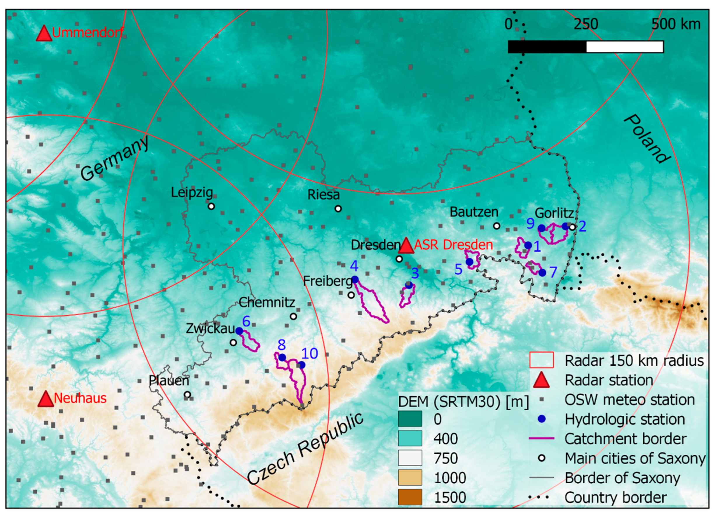
Figure 1. An overview of the study region, Saxony, Germany (WGS-84 Pseudo-Mercator projection), with a background of a digital elevation model (DEM) based on SRTM30. Presented are also radar stations of DWD, recording meteorological station from OSW and the ten selected catchments. The ID numbers of the catchments here match those in Table 1.
Hydrology 09 00204 g001
Figure 2. The distances (calculated as boxplots) of the meteorological sensors: precipitation from gauges (P), global radiation (Rn), temperature (T), and wind speed (Wind) from the centroids of the catchments in the OSW. Note the difference in scales used for the vertical axis.
Hydrology 09 00204 g002
Figure 3. An overview of the model setup, exemplified for the Kreischa catchment: (a) a topographic map based on the digital elevation model STRM30, (b) land use map simplified from CORINE2012, (c) soil map simplified from BK50, (d) RADKLIM-RW exemplary for one hour and meteorological stations available from OSW.
Hydrology 09 00204 g003
Figure 4. Relative difference between the monthly corrected precipitation after Richter correction for the OSW and RADKLIM datasets in the period 2006–2017.
Hydrology 09 00204 g004
Figure 5. Principal scheme of the validation process.
Hydrology 09 00204 g005
Figure 6. The absolute difference between annual precipitations derived from OSW and RADKLIM for the ten selected catchments in the study period 2006–2017.
Hydrology 09 00204 g006
Figure 7. The average differences of monthly precipitations from OSW and RADKLIM for the ten selected catchments in the study period (2001–2017).
Hydrology 09 00204 g007
Figure 8. The correlation of daily precipitation from OSW and RADKLIM for the ten selected catchment in the study period (2001–2017) within the value range from 0 to 50 mm/day. Two seasons were examined, namely summer (red points) and winter (blue points).
Hydrology 09 00204 g008
Figure 9. Monthly average of water balance components (precipitation (P), discharge (Q), evapotranspiration (ET), and soil moisture content (SM)), exemplary for Holtendorf catchment (above) and Niederoderwitz catchment (below) in the period 2001–2017.
Hydrology 09 00204 g009
Figure 10. Exemplarily results of simulated (weighted mean from all HRUs) runoff derived from four different precipitation datasets (OSW uncorrected, OSW corrected, RADKLIM uncorrected, and RADKLIM corrected) compared to the observations for the ten selected catchments, exemplary for 2017.
Hydrology 09 00204 g010
Figure 11. Skill scores of observed and simulated discharge with different precipitation data inputs for the ten selected catchments on a monthly scale.
Hydrology 09 00204 g011
Figure 12. Low (90th percentile), medium (50th percentile), high (10th percentile), and extreme (1st percentile) flow simulated with gauge and radar precipitation with and without Richter corrections.
Hydrology 09 00204 g012
Table 1. Summary of the important characteristics of selected catchments.
Water Gauge
ID
Area (Km²)Average
Elevation
(m.a.s.l.)
HRU/
Km²
Land Use (%)
Agriculture Grass
Land
Deciduous
Forest
Evergreen
Forest
Other
Großschweidnitz141.44239.667.2472121812
Holtendorf254.17269.293.465132137
Kreischa343.88384.9111.244254225
Krummenhenners-dorf4130.92476.964.05729059
Neustadt540.18386.167.7302442814
Niedermuelsen649.58355.619.7472111813
Niederoderwitz728.87123.803.153182423
Niederzwoenitz831.36600.582.8291604411
Reichenbach- Oberlausitz942.51266.056.26418369
Tannenberg1091.48662.024.3242314210
Table 2. Average days for each type of precipitation classified with mean temperature (Appendix C) for the ten selected catchments in the period 2001–2017.
Water Gauge/IDAverage Annual Days of
SnowSleetRain
Großschweidnitz14048277
Holtendorf24149275
Kreischa34250273
Krummenhenners-dorf44452269
Neustadt54551269
Niedermuelsen64149275
Niederoderwitz74350273
Niederzwoenitz84354268
Reichenbach- Oberlausitz93846282
Tannenberg107059236
Table 3. Precipitation difference for the study catchments on the different time scales of gauge versus radar using Wilcoxon–Mann–Whitney statistics test.
Water GaugeDailyMonthlyAnnual
Großschweidnitz5.6 **−1.5 0.3
Holtendorf40 **25 **22.1 **
Kreischa22.5 **3.5 **6.5 **
Krummenhenners-dorf19.7 **−0.9 0.2
Neustadt6.9 **−5.8 **−8.8 **
Niedermuelsen27.9 **7.7 **7.4 **
Niederoderwitz20.6 **0.3 0.8
Niederzwoenitz33.8 **8.2 **7.9 **
Reichenbach- Oberlausitz32.0 **14.5 **9.7 **
Tannenberg35.1 **10.5 **8.3 **
** significant: p value < 0.05.
Publisher’s Note: MDPI stays neutral with regard to jurisdictional claims in published maps and institutional affiliations.