Flood Exposure Assessment and Mapping: A Case Study for Australia’s Hawkesbury-Nepean Catchment

Abstract

Floods are the most common and costliest natural disaster in Australia. However, the Flood Risk Assessments (FRAs) employed to manage them are hazard-focused and tend to overlook exposure and vulnerability. This leaves potential for Australian FRAs to make better use of a technique which holistically incorporates all three flood risk components. In this study, flood exposure assessment and mapping for the Hawkesbury-Nepean Catchment (HNC), a flood-prone region in Australia, was conducted. Three flood exposure indicators—population density, land use type, and critical infrastructure density—were selected to derive the flood exposure index (FEI). Results demonstrated that Statistical Areas Level 2 (SA2s) on or near the floodplain, located near the eastern border of the HNC, are severely or extremely flood-exposed due to the significant presence of flood-exposed assets such as hospitals or police stations. The Wahroonga (West)—Waitara SA2 was the most exposed SA2 in the catchment (extreme exposure). This was followed by the Acacia Gardens, Glendenning—Dean Park, and Cambridge Park SA2s (all severely exposed). The Goulburn SA2 was also identified as severely flood-exposed even though it remains outside of the floodplain. This is due to its many exposed assets as Australia’s first inland town. All selected indicators were found to either strongly or moderately positively correlate with the FEI. Ultimately, this novel FEI can assist in the reduction of flood risk in the HNC, as well as foster community resilience strategies. Additionally, the developed scalable and replicable methodology can be applied to other flood-prone regions of Australia.

1. Introduction

1.1. Floods as a Natural Hazard

Described as “an overflow of water beyond the normal limits of a watercourse” [1], floods have become a recognisable symbol throughout Australian history. They are frequently described as the most common and costliest natural disaster [2]. Flood events such as the 2010–2011 Queensland floods, as well as the recent 2022 floods along the eastern coast of the country, have demonstrated that Australia is not unaccustomed to floods and their destructive socioeconomic costs.

There are three major types of floods: fluvial floods (inland riverine flooding), pluvial floods (inland flash flooding or overland flooding), and coastal inundation (coastal flooding due to storm surge) [3]. From an environmental perspective, these floods are an important component of natural ecosystems because they spread silt and nutrients on floodplains to support vegetation and wildlife [4]. However, the floods which are associated with community and economic disruption in Australia are primarily caused by three major factors. These are: natural variability of key climate drivers such as the El Niño-Southern Oscillation, increasing impacts of climate change, and ongoing urbanisation on floodplains, as described by the Intergovernmental Panel on Climate Change [5]. These factors are also interrelated in the sense that the frequency and intensity of one of these factors can affect the others.

An understanding of flood risk can come from natural hazard risk. The IPCC defines natural hazard risk as “the potential for adverse consequences for human or ecological systems” [5]. Natural hazard risk can be conceptualised through the ‘natural hazard risk triangle’ [6,7]. The risk triangle presents natural hazard risk as the product of three subcomponents: hazard (the natural hazard itself), exposure (what stands to be lost to the natural hazard), and vulnerability (characteristics of the environment which exacerbate the natural hazard event).

The risk triangle can be applied to a flood context in which flood risk is represented by flood hazard, exposure, and vulnerability; this has applications in Flood Risk Assessments (FRAs). FRAs built upon the risk triangle framework can help to understand the flood risk of areas based on exposed or vulnerable elements in relation to hazard. This assists decision makers and local authorities by identifying high flood risk areas, allowing them to prioritise specific flood-prone areas and their communities.

Local- and state-FRAs in Australia abide by best practice flood management guidelines outlined by the Australian Institute for Disaster Resilience; however, the hydrological modelling outputs of these FRAs are typically flood hazard-focused, with less emphasis on flood exposure or vulnerability [8]. A more robust approach to Australian FRA could be achieved through risk assessment using indices. An index within a flood risk context involves condensing large volumes of data into standardised integer values across a given area based on carefully selected indicators. Such indicator-based approaches are also referred to as Multi-Criteria Decision Making (MCDM) techniques, especially during the data standardisation phase (e.g., [9]). Indicators exist as proxies for the spatial and temporal conditions over a given area. Through this, each area is assigned a single value to characterise its flood risk.

Indices have rarely been used to assess inland flood risk in Australia. In earlier Australian FRAs studies, flood risk was assessed in core suburbs of the Local Government Area of Brisbane City, in the context of the 2010–2011 Queensland floods [10], and in Melbourne, also at an Local Government Area level, with a focus on flood vulnerability [11].

Indices are a useful approach to FRA because they are scalable, replicable, and quantitative in nature. They have the potential to provide a more holistic insight into flood risk by assessing all of flood hazard, exposure, and vulnerability. Crucially, the effectiveness of an FRA can be determined in part through the ability for its method to be replicated elsewhere. Index-based FRAs can achieve this more easily than modelling outputs, particularly because they are less resource intensive. For these reasons, indices can be a powerful novel technique in assessing flood risk in Australia.

This study focuses on flood exposure within flood risk. However, it is important to understand the overall context in which flood exposure exists. Flood hazard, exposure, and vulnerability are defined widely and inconsistently in the relevant literature (see

Table A1. Examples of flood exposure definitions present in the literature. Note that flood exposure can be defined widely and inconsistently, therefore characterising it accurately is important to establish appropriate context for this study (this study assumes the Intergovernmental Panel on Climate Change definition).

Source	Definition
United Nations International Strategy for Disaster Reduction (2009)	The people, property, systems, or other elements present in hazard zones that are thereby subject to potential losses.
Kundzewicz and Stoffel (2016)	The assets and populations at risk; the presence of people, livelihoods, or ecosystems… in places and settings that could be adversely affected by floods.
Nasiri et al. (2016)	People and their surroundings and every element present in flood-prone area being exposed to the flood impacts as a subject to potential losses.
United Nations Office for Disaster Risk Reduction (2020)	The assets of interest and at risk (such as the environment, the economy, buildings, or people); the situation of… tangible human assets located in hazard-prone areas.
Membele et al. (2022)	The probability that people or physical items will be impacted by floods.
Ming et al. (2022)	At-risk elements such the types, characters, and values of the properties or buildings that are under threats of flooding.
IPCC (2022)	The presence of people; livelihoods; services and resources; infrastructure; or economic, social, or cultural assets in places and settings that could be adversely affected by a flood event.

, Appendix A for different characterisations of flood exposure). For this study, IPCC definitions have been used within a flood context [5], defining flood exposure: “The presence of people; livelihoods; services and resources; infrastructure; or economic, social, or cultural assets in places and settings that could be adversely affected by a flood event”.

It should be noted that flood exposure and vulnerability are typically characterised similarly in the literature (e.g., [12,13]). The IPCC defines flood vulnerability as “the propensity or predisposition to be adversely affected by a flood event, encompassing a variety of concepts and elements including sensitivity or susceptibility to harm and lack of capacity to cope and adapt” [5]. Outside of the IPCC definitions provided, flood exposure refers to elements of a community which stand to be lost to flood (such as people, shelter, food, or support services), and flood vulnerability refers to characteristics of a community which have the potential to affect overall flood risk (e.g., a house’s elevation above sea level). Distinguishing between flood exposure and vulnerability so that flood exposure could be assessed alone was crucial to this study’s aims and objectives.

1.2. Research Aims and Objectives

The research question which prompted this study was: How can the inland flood exposure of at-risk communities be most accurately assessed using an index-based approach? The aim of this proof-of-concept was then to develop a methodology for flood exposure assessment and to map a flood exposure index (FEI), within the context of an overall flood risk index, in an Australian case study area. The Hawkesbury-Nepean Catchment (HNC) was chosen as this study area because it is significantly flood-prone.

Importantly, an indicator-based method to assess flood hazard risk in the HNC has been developed in [14] and a Flood Hazard Index (FHI) was created. Examining a significant flood event in the HNC in March 2021, it was found that nearly 85% of the HNC was classified by the FHI at the ‘severe’ or ‘extreme’ levels. The urbanised floodplain area in the central-east of the HNC had the highest FHI values. Conversely, regions along the western border of the catchment had the lowest flood hazard.

Additionally, further investigation of an indicator-based approach to flood vulnerability assessment using indicators which represent environmental and socioeconomic characteristics has been conducted in [15]. It was found that flood vulnerability was at its highest in the HNC floodplain region on the outskirts of Greater Western Sydney.

By examining key components of an overall flood risk index in the HNC, earlier studies have developed methodologies for flood hazard assessment [14] and flood vulnerability assessment [15]. By applying indicator-based methods, this research also represents a novel approach to Australian flood exposure assessment which may be replicated elsewhere to produce similar outputs unique to any given area.

The aim and objectives of this research support future research—creating an overall flood risk index based on flood hazard, exposure, and vulnerability indices. It may also be used to inform community flood resilience, as well as other flood risk management approaches such as flood early warning systems. This study can assist in the overall reduction of flood risk in the HNC alongside hazard and vulnerability analyses, as well as act as a strong example of a FRA which employs the novel approach of an index in order to quantitatively analyse flood-exposed assets in a community. It can also contribute to flood resilience analyses, which aim to assess coping, restoring, and adapting to future floods.

2. Materials and Methods

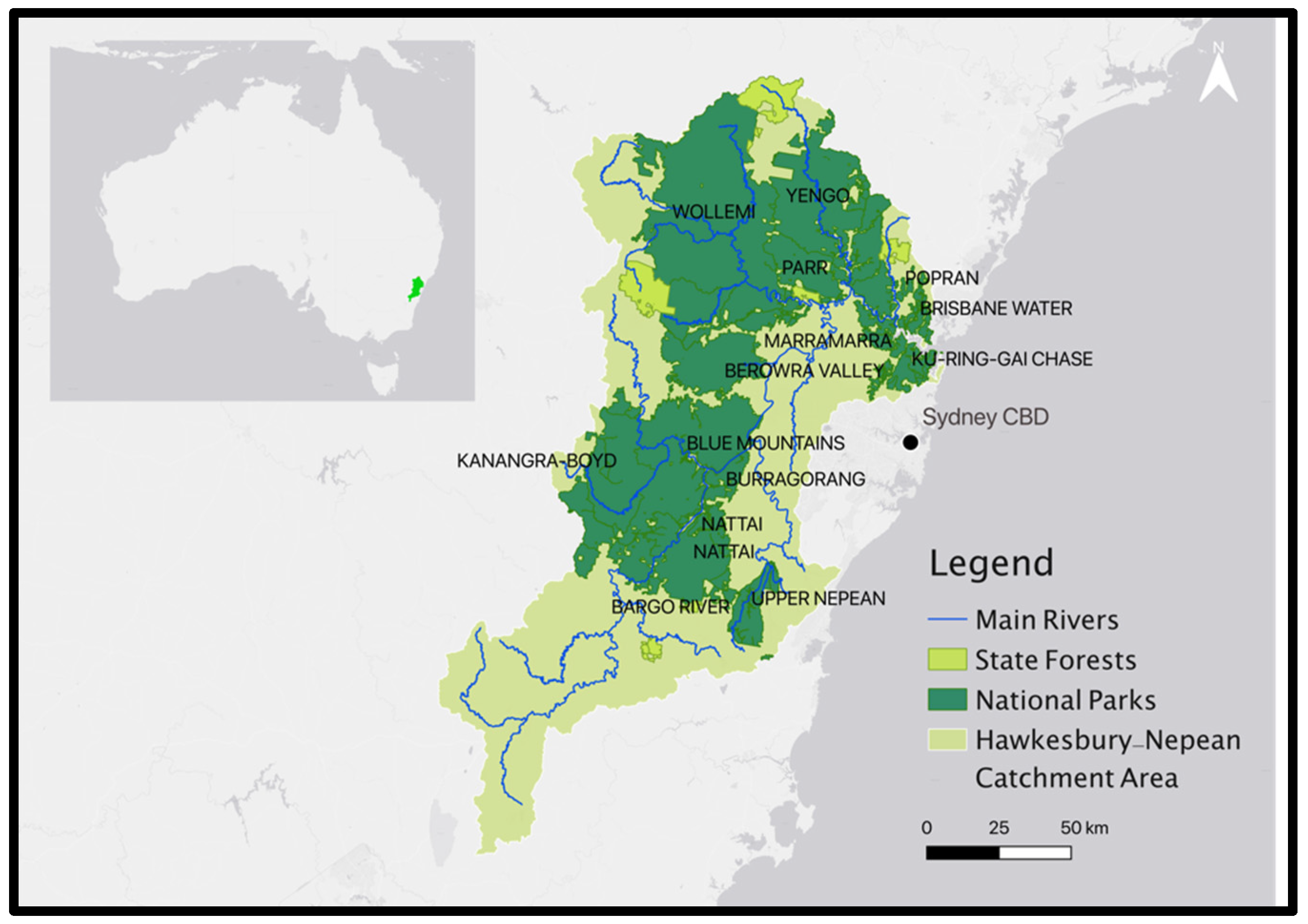
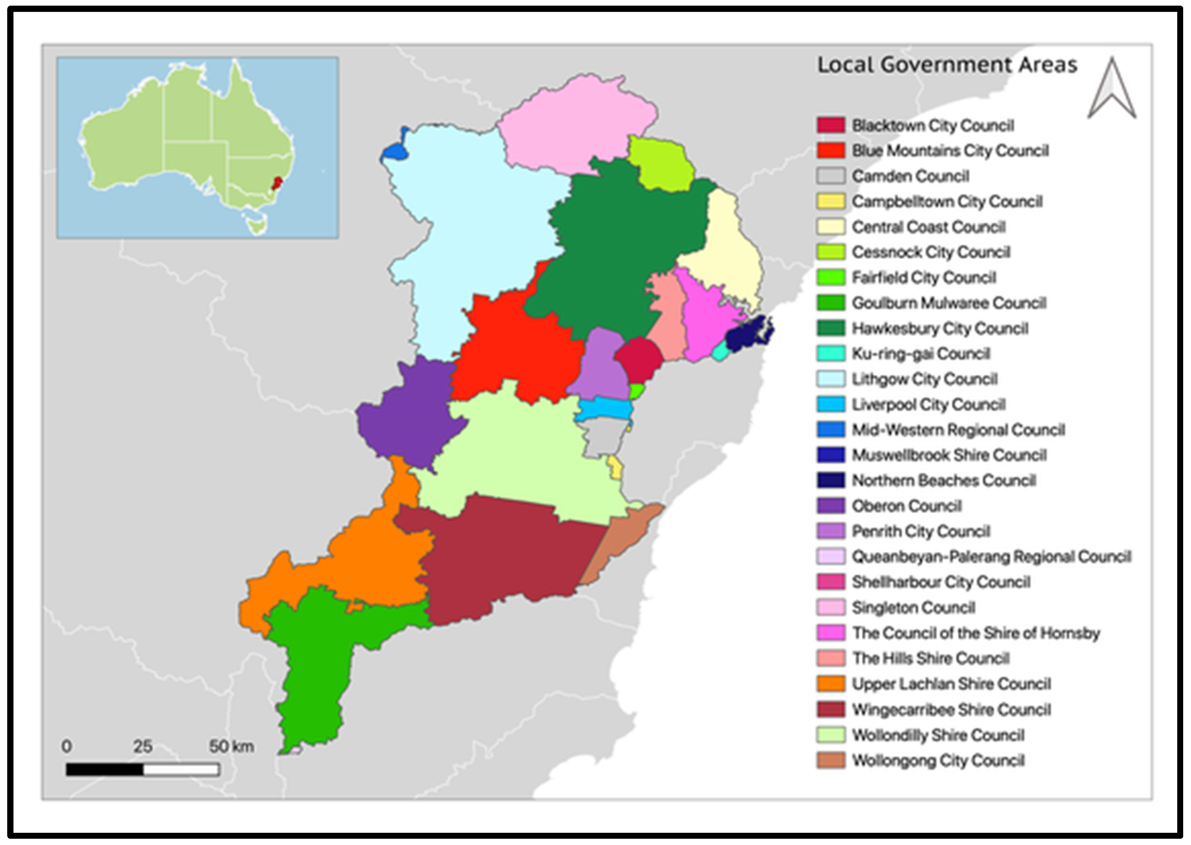
2.1. Study Area

The study area is the Hawkesbury-Nepean Catchment (HNC) (Figure 1). The HNC provides water, food, and other valuable resources to twenty-six Local Government Areas (for detail, see Figure A1, Appendix B), some of which are in the broader Greater Western Sydney area to the west of the Sydney CBD.

The HNC’s communities are at significant risk of flooding. According to [16], the HNC is the highest flood risk area in NSW. Due to a growing population, [16] also claims that the catchment has the greatest flood exposure in NSW, if not Australia. This is because the majority of the catchment’s growing population (up to approximately 134,000 people) lives on or near the floodplain. Similarly, over 25,000 residential properties and approximately two million square metres of commercial space are exposed to flood [16]. This results in the annual average cost of flood damage in the catchment being over approximately AUD 70 million (adjusted for 2022 inflation) [17].

The FEI designed in this study prioritised human health and livelihoods in accordance with the adopted IPCC exposure definition. Likewise, it only considered flood exposure in the context of inland flooding, not coastal inundation. This is because coastal inundation is caused by another natural hazard—storm surge. Accordingly, only fluvial and pluvial flood exposure in the HNC were considered. It should finally be noted that this is the first proof-of-concept FEI to make use of the HNC as the study area of interest, being one of the most flood-prone areas in Australia.

2.2. Flood Exposure Indicators

Three indicators were chosen to characterise flood exposure: population density, land use type, and critical infrastructure density. These indicators were selected as suitable proxies having considered the literature with similar methodologies and scope. As importantly, these three indicators align with specific characteristics of the HNC. In recent years, rapid urban growth has occurred throughout the catchment, alongside the development of diverse economies. This has resulted in a growing population, as well as land use types and critical infrastructures related to urban growth (such as cropping lands or locations of emergency services, respectively), for which a high annual gross regional product of approximately AUD 104 billion exists [16]. For this reason indicators of population density, land use type, and critical infrastructure density capture the urbanised yet flood-exposed HNC for a proof-of-concept FEI. Ultimately, these indicators succeed in characterising the flood-exposed elements of the HNC, namely, people and their built environment, so that actionable results can be drawn upon for future work.

Vegetation cover density was also initially considered as a potential indicator to characterise flood exposure. Vegetation cover density refers to the spatial distribution of vegetation in a community (being standardised between differently sized regions). This indicator was considered because a community’s vegetation cover plays a significant role during a flood event, therefore capturing its flood exposure is likely to be important. Vegetation cover can disrupt surface water discharge by acting as a physical barrier, absorbing water, or changing soil structure to increase its water-holding capacity. However, it typically only describes natural green cover rather than urban development-related green cover. Furthermore, vegetation cover density does not capture the broader socioeconomic flood-exposed elements sought by this study. Since a community focus was the priority of this study, this indicator was excluded from the final FEI.

The following sections explain the justification behind the choice of each selected indicator.

2.2.1. Population Density

Population density is commonly used as an indicator of population exposure in FRAs (e.g., [18,19]). It can be calculated by dividing an estimated resident population (typically obtained via census data) by land area. Population density is positively correlated with flood exposure; an increase in population density results in more people impacted in the presence of a flood event which in turn results in greater flood exposure.

2.2.2. Land Use Type

Land use type is also commonly employed as a flood exposure indicator (e.g., [18,20]). Land use type describes the different land types which exist in a given area based on their use (e.g., irrigated cropping, housing, wetland, or mining). These land types are then typically associated with community value in the context of flood exposure. For example, built infrastructure is typically said to have more community value than minimal use lands because if infrastructure were to be lost to flood, it would most likely result in greater costs to the community. Land use type can be correlated with flood exposure by assigning a value to each land use type (e.g., [21]), where higher values indicate more community value and thus greater flood exposure (such land use type reclassification will be conducted for this study—see Section 2.3.2). Evaluating land use type is important because different land use types contribute to flood exposure to different extents. It should be noted that this indicator can also characterise flood vulnerability (e.g., [19,22,23]). The aim was to avoid this overlap; Appendix C has further information on flood exposure and vulnerability comparisons.

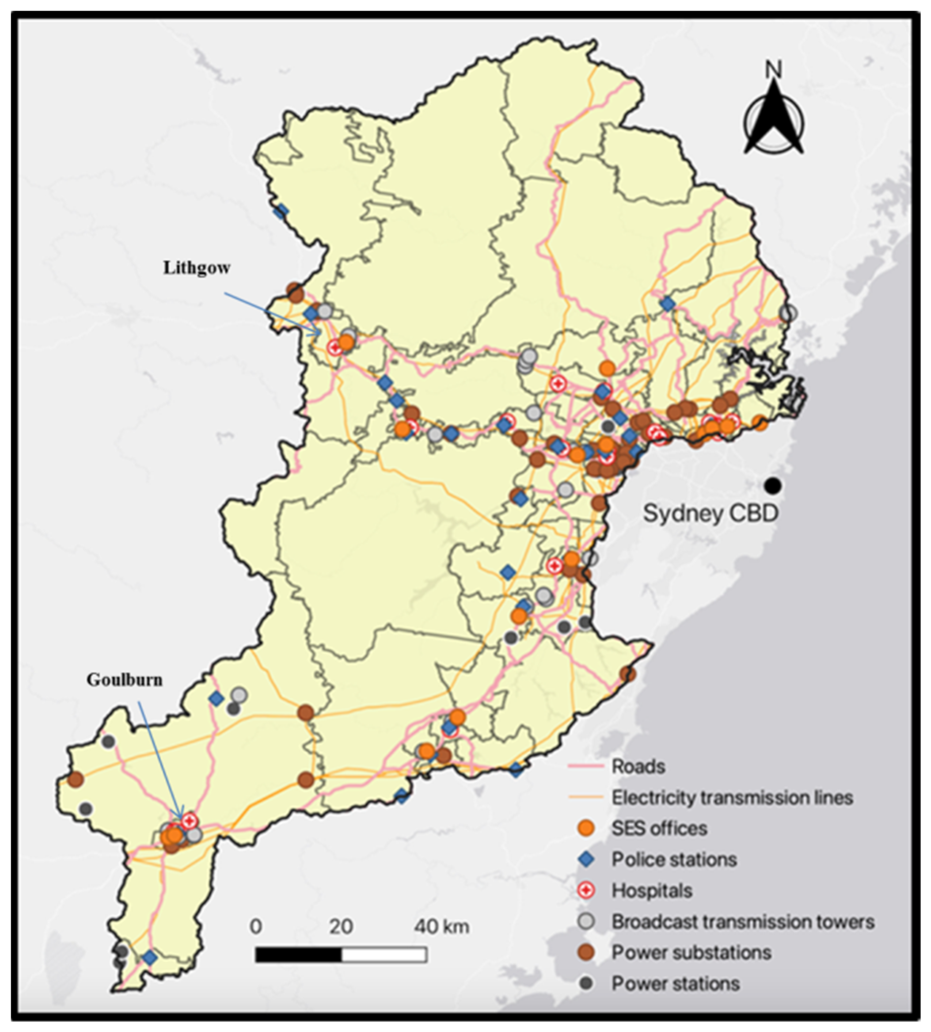
2.2.3. Critical Infrastructure Density

Critical infrastructure (CI) density describes the amount of CI per land area within a community. This indicator is well-characterised in the literature as being important to assess in the context of flood (e.g., [24,25]). This research includes eight CIs (described as sub-indicators): roads (including State Emergency Service [SES] evacuation routes), power stations, power substations, electricity transmission lines, hospitals, police stations, SES offices, and broadcast transmission towers. These describe services, industries, and utilities most important to a community such as transport, energy, emergency services, and communication. It should be noted that cell towers, as a type of broadcast transmission tower, were excluded from this indicator due to data availability difficulties. Cell towers are critical for cellular communication during a flood event, and so this leaves potential for future work.

CI density is positively correlated with flood exposure—an area with more CIs has greater flood exposure. In a similar manner to land use type, this is an essential indicator for this study because a community’s CI and their potential losses during flood events greatly contribute to flood exposure and overall flood risk.

2.3. Data

Metadata for flood exposure indicators comprising the final FEI are given in

Table A2. Datasets and other relevant metadata for each of the three indicators in this study. Note that, following the population density and land use type indicators, data relates to sub-indicators within the critical infrastructure density indicator. All indicators were covered by a CC BY 4.0 licence. The two sub-indicators which were covered by a CC BY-NC 4.0 licence specifically are marked with an *.

Indicator/ Sub-Indicator	Dataset	Source	Original Resolution	Year
Population density	Regional population estimate	ABS	SA2 polygon vector	2021
Land use type	NSW Landuse 2017 v1.2	NSW Government	50 m raster	2017
Roads	GEODATA TOPO 250K Series 3	Geoscience Australia	50 m polyline	2006
Power stations	Foundation Electricity Infrastructure	Geoscience Australia	50 m point	2021
Power substations	Foundation Electricity Infrastructure	Geoscience Australia	50 m point	2021
Electricity transmission lines	Foundation Electricity Infrastructure	Geoscience Australia	50 m polyline	2021
Hospitals	MyHospitals database	Australian Government AIHW	50 m point	2022
Police stations *	ArcGIS Online	ArcGIS Online	50 m point	2021
SES offices *	ArcGIS Online	ArcGIS Online	50 m point	2019
Broadcast transmission towers	Broadcast Transmitter Data (AM Radio, FM Radio, Digital TV, Digital Radio, and current and future temporary transmitters)	Australian Government ACMA	50 m point	2017

, Appendix D.

The population density and CI density indicators were available at Statistical Area Level 2 (SA2). According to [26], SA2s are “medium-sized general purpose areas”, with each representing “a community that interacts together socially and economically”. This community-focused representation was important when seeking to characterise these indicators. Data at SA2 was also readily available and of a high enough resolution to provide insightful results. Hence, the final flood exposure index was mapped at SA2. However, the land use type indicator was not mapped at SA2 because a higher resolution 50 m raster dataset was available (see Table A2, Appendix D), which better represented land use exposure in the catchment.

2.3.1. Population Density

The population density indicator was created using QGIS 3.24 software. An SA2 population estimate dataset was downloaded from the ABS as a GeoPackage; this vector was imported into QGIS and cut to HNC boundaries. Population density was then visually presented in terms of people per SA2 and subsequently rasterised.

2.3.2. Land Use Type

The land use type indicator was created using ArcGIS 10.7 software. NSW Government’s Landuse 2017 v1.2 dataset was downloaded as a shapefile; this 50 m raster was then imported into ArcGIS and cut to HNC boundaries.

This clipped dataset contained thirty-one land use types (

Table A3. All thirty-one land use types present in the NSW Landuse 2017 v1.2 dataset; the eight reclassified land use type categories are also provided in italics above the land use types that were used to create them.

Other Other minimal use Land in transition Irrigated land in transition Water bodies Lake Reservoir/dam River Channel/aqueduct Estuary/coastal rivers Nature conservation Nature conservation Managed resource protection Marsh/wetland Cropping Cropping Irrigated cropping Grazing Grazing native vegetation Grazing modified pastures Grazing irrigated modified pastures

Forestry Production native forestry Plantation forests Irrigated plantation forests Horticulture Perennial horticulture Seasonal horticulture Irrigated perennial horticulture Irrigated seasonal horticulture Intensive horticulture Infrastructure Intensive animal production Manufacturing and industrial Residential and farm infrastructure Services Utilities Transport and communication Mining Waste treatment and disposal

, Appendix E). However, it was important to characterise land use type more suitably because each land use type was then visualised with a respective flood exposure value associated with it. The thirty-one land use types were reclassified into a subset of eight: water bodies, nature conservation, forestry, cropping, grazing, horticulture, infrastructure, and ‘other’ [27]. Such land use reclassification is commonly seen in the literature (e.g., [28,29]). Although it can be said that this reclassification approach introduces some level of subjectivity to analysis, it was conducted based on a comprehensive understanding and informed decisions related to land use types within the study scope. Therefore, it was deemed suitable for this study.

A value was then assigned to each reclassified land use type to give them an exposure rating to flooding, based on the extent to which they may be flood-exposed in the catchment. This is presented in

Table 1. Reclassified land use types, with respective values and ratings, for the land use type indicator.

Classification	Value (Weight Assigned)	Rating
Other	0.1	Very low
Water bodies	0.1	Very low
Nature conservation	0.5	Moderate
Forestry	0.5	Moderate
Cropping	0.7	High
Grazing	0.7	High
Horticulture	0.7	High
Infrastructure	0.9	Very high

. The weighting of reclassified land use types was based on prior literature and the land use type’s significance to the communities in the HNC. Appendix F explains how such weights were assigned, as seen in Table 1. For example, infrastructure was weighted as 0.9 because it is the flood-exposed built environment and this study scoped such. In contrast, water bodies were weighted as 0.1 because it is argued that they, for the most part, represent flood hazards themselves and so do not stand to be lost.

The final output was then a reclassified land use type raster layer, with each of the eight classifications being associated with a particular flood exposure value and rating.

2.3.3. Critical Infrastructure Density

The critical infrastructure density indicator was created using QGIS 3.24 and ArcGIS 10.7 software. Datasets were downloaded as shapefiles (see Table A2, Appendix D for data sources); these vectors were imported into QGIS and cut to HNC boundaries. Importantly, datasets for power stations, power substations, hospitals, police stations, SES offices, and broadcast transmission towers represented point data, and datasets for roads and electricity transmission lines represented polyline data.

Having imported datasets, duplicates were removed from hospital and broadcast transmission tower data layers in QGIS. In addition to the dual carriageways, principal roads, and secondary roads represented by the roads data layer, SES-recommended evacuation routes were included via QGIS. Capturing these was essential as they represent key transport routes in emergency situations [16]. These evacuation routes are located throughout the built-up areas of Wallacia, Penrith, Richmond, Windsor, and Blacktown.

For each of the six point data layers, the number of CIs per SA2 was calculated, and the CI density was calculated by dividing these sums by SA2 land area. For the two polyline data layers (roads and electricity transmission lines), the total length associated with the polyline data was calculated per SA2. One data layer with length sums per SA2 from these two data layers was generated, and the CI density for the polyline data was calculated by dividing these sums by SA2 land area.

On ArcGIS, both the point and polyline CI density data layers were normalised to be between 0 and 1 so that they could then be merged together while being equally weighted. The final data layer was then converted into a raster layer.

CI density, in particular, was calculated because SA2s in the HNC vary significantly in size. A simple count of the CI sub-indicators would not be representative of CI distribution taking into account differently sized-SA2s. CI density is a way of standardising between these SA2s.

2.4. Index Calculation and Mapping

Standardising was required because the collected data varied significantly in unit and quantity between indicators (population density as people per km², land use type as reclassified integer values, and CI density as normalised 0–1 values). Data standardising allowed flood exposure indicator maps to be combined into a final FEI map.

Data was standardised using ArcGIS’ fuzzy membership tool, which is commonly used for index-based FRAs (e.g., [30]). Fuzzy membership involves 0–1 standardising by assigning membership classes. All three indicators were assigned the fuzzy large membership class, because greater values for each indicator related to greater flood exposure. Having done this for each indicator, values above a certain midpoint were weighted more strongly and values below less strongly, with a respective spread (the midpoint and spread being unique to each indicator).

ArcGIS’ Fuzzy Gamma Overlay function was used to combine the three fuzzy maps into a final FEI map. Fuzzy Gamma Overlay is an equal weighting technique which involves multiplying together fuzzy sum and fuzzy product methods, taken to the power of a certain gamma value (Equation (1)). For this study, a general gamma value of 0.9 was used (being the industry standard, e.g., [30]).

µ_gamma = (µ_sum)^γ × (µ_product)^1−γ

(1)

After creating the FEI, it was important to conduct a correlation analysis to determine the spatial similarity between the population density, land use type, and critical infrastructure density indicators, as well as between each of these indicators and the FEI. Doing so provided a statistical insight into each indicator’s relationship with flood risk.

The correlation analysis was conducted using Python programming language (specifically, the SciPy Python library). All four data layers (that of the three indicators and the FEI) were imported into Python as NetCDF files, visualised, interpolated to a common size, and correlated using the Python library.

3. Results

For assessment and mapping of individual indicators and overall flood exposure in the HNC, five risk classes were assigned to fuzzified values: very low, low, moderate, severe, and extreme (

Table 2. Risk classes assigned to fuzzy values for flood exposure indicator maps and the overall flood exposure index map.

Risk Class	Population Exposure Values	Land Use Exposure Values	Critical Infrastructure Exposure Values	Flood Exposure Index Values
Very low	0.001–0.247	0.0003	0.000–0.241	0.001–0.247
Low	0.248–0.494	-	0.242–0.483	0.248–0.494
Moderate	0.495–0.742	0.5000	0.484–0.725	0.495–0.742
Severe	0.743–0.989	0.8432	0.726–0.967	0.743–0.989
Extreme	0.990	0.9497	0.968	0.990

). Note that the ‘low’ risk class was not used for land use exposure as such values represented four distinct reclassified categories—not five. This is because four categories resulted after assigning values and ratings to each reclassified land use type (e.g., both nature conservation and forestry were assigned a value of 0.5; see Table 1).

A map of population flood exposure in the HNC (Figure 2) demonstrates that SA2s on or near the catchment’s floodplain as well as some SA2s in the broader Greater Western Sydney area have moderate, severe, or extreme population exposure. Very low or low population exposure was observed outside of this area, away from the floodplain. Importantly, lower exposure is comparative; this does not suggest that SA2s have absolute low population exposure but rather that, relative to other SA2s, their exposure is lower. Notable exceptions were the Goulburn SA2, the Calga—Kulnura SA2, and SA2s including and around Bayview—Elanora Heights (annotated). These areas, although away from the floodplain, presented moderate, severe, and extreme population exposure, respectively (annotated).

A map of land flood exposure in the HNC (Figure 3) shows that SA2s on the catchment’s floodplain, as well as surrounding SA2s throughout Greater Western Sydney, have extreme land use exposure. Extreme land use exposure was also observed in a region between Blue Mountains National Park (BMNP), as well as in the Goulburn SA2 which is far from the catchment’s floodplain (annotated). Furthermore, SA2s associated with severe land use exposure appeared to surround most extremely exposed areas, as well as the southern part of the catchment. Moderate land use exposure was seen in central and northern areas of the catchment, and very low land use exposure sporadically throughout the catchment. Very low land use exposure was due to either water bodies or minimal use lands. Broadly, very low land use exposure on or near the floodplain was associated with water bodies, with exposure outside of the floodplain being associated with minimal use lands.

A map of CI flood exposure in the HNC (at SA2), after fuzzy standardisation in presented in Figure 4. The map shows that some SA2s on or near the HNC’s floodplain have extreme CI exposure. Surrounding SA2s then presented moderate and severe CI exposure. Note that the Goulburn and Lithgow SA2s, as well as a region between Blue Mountains National Park, presented moderate to severe CI exposure, even though they are far from the floodplain (annotated). Very low or low CI exposure was seen outside of these areas.

A map of the final FEI in the HNC based on three indicators—population density, land use type, and critical infrastructure density—is presented in Figure 5 at 50 m resolution within SA2 boundaries. The map demonstrates that, in general, it is the SA2s on or near the HNC’s floodplain that have extreme flood exposure.

As per Figure 5, all of the eastern region of the catchment which surrounds the Sydney CBD presented moderate or severe flood exposure. One key exception is the Goulburn SA2 (annotated). Goulburn displayed severe exposure in the far south-east of the floodplain. Ultimately, most of the catchment showed low, moderate, severe or extreme flood exposure, with urbanised SA2s in the Greater Western Sydney region presenting higher flood exposure—particularly those on or near the catchment’s floodplain.

Correlation analysis results for the three flood exposure indicators for the HNC was conducted. Each indicator was spatially correlated against the final FEI. It was found that the population density indicator spatially correlated to the FEI the most (R = 0.72, p < 0.0001), followed by the critical infrastructure density indicator (R = 0.67, p < 0.0001), and the land use type indicator the least (R = 0.51, p < 0.0001). All indicators were positively correlated to the FEI.

4. Discussion

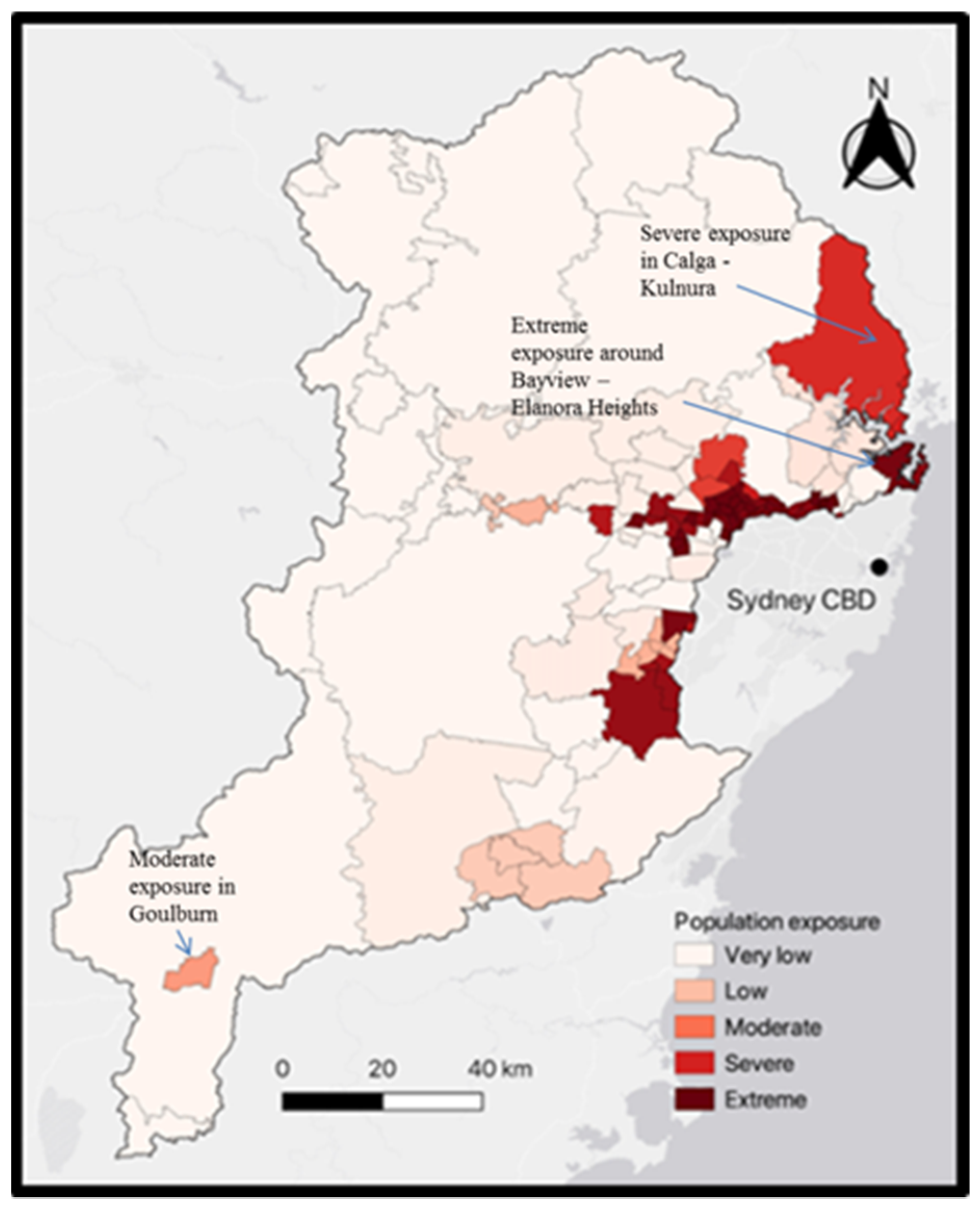
4.1. Population Exposure

4.1.1. Population Exposure Patterns

A map of population flood exposure (Figure 2) demonstrates that populations on or near the HNC’s floodplain have extreme flood exposure. More broadly, all of Greater Western Sydney presented moderate, severe, or extreme flood exposure. This appears to be representative of Greater Western Sydney’s rapid urban growth and therefore population dense SA2s [16]. In contrast, the very low or low flood exposure seen to the west of the catchment represents SA2s which are sparsely populated, due to their being far away from Greater Western Sydney and the Sydney CBD. Ultimately, these flood exposure trends are consistent with Greater Western Sydney’s urban growth, being in proximity to the Sydney CBD. With urbanisation comes population growth [31], and thus higher population exposure in the presence of inland flooding.

As per the population exposure output for this study, the Goulburn, Calga-Kulnura, and Bayview—Elanora Heights SA2s presented higher than expected population exposure, considering their location away from the catchment’s floodplain and more urbanised areas. Goulburn’s moderate population exposure can be attributed to its historic origins, being Australia’s first inland town. As thus, its estimated resident population and respective population exposure have been allowed to increase steadily over time. This also aligns with the key findings from the FHI relevant to this study and the HNC [14]; Goulburn has two converging nearby rivers which present extreme flood hazard in the context of the case study. Calga-Kulnura’s severe exposure appears to be in part due to its tourism origins. Since the late 1800s, its tourism industry has expanded greatly, with land closer to the eastern coast being used for holiday villages and resorts [32]. This, in addition to its favourable location near the coast and the Sydney CBD, results in significantly high population density relative to other SA2s. Finally, the extreme exposure seen in Bayview—Elanora Heights can, for the most part, be attributed again to it being a favourable coastal location that encourages urban development, bolstering its estimated resident population.

It should be noted that the connection between rapid urban growth and increasing flood risk is well-established in the literature. For example, a 2021 FRA of Delhi, India, scoped urban flood-prone areas and found that one of the main causes of flooding was inefficient urban drainage systems, thereby increasing flood risk [33]. A study from Ontario, Canada, also claimed that urbanisation generally reduces hydrologic response time [34]. A catchment’s hydrologic response describes how quickly it can react to a flood event. A reduced hydrologic response results in a catchment counteracting flooding less quickly, thereby increasing flood risk. Through this, there is a strong link between urbanisation and increasing flood exposure as a component of risk.

4.1.2. Population Density Indicator Analysis

It was important to utilise a population density indicator as opposed to an alternative such as an estimated resident population indicator because population density can standardise data between differently sized SA2s (e.g., [35]). Crucially, though, by presenting population density at SA2, there was potential for smaller SA2s in the catchment to be given higher population exposure values, and larger SA2s lower values (regardless of their estimated resident populations). This is because estimated resident populations would be divided by smaller and larger land areas, respectively. Although acknowledged as a constraint of this study, population density at SA2 still provided suitable results to draw upon, because this constraint would not produce noticeable and statistically significant outliers.

The fuzzy midpoint and spread used to standardise population density data were 500 and 2, respectively (see

Table A4. Fuzzy midpoints and spreads for each flood exposure indicator, for ArcGIS’ fuzzification of initial data layers.

Indicator	Fuzzy Midpoint	Fuzzy Spread
Population density	500 people/km2	2
Land use type	50 (integer value)	5
Critical infrastructure density	0.2 (0–1 normalised)	2

, Appendix G, for a summary of such fuzzy information). This produced a fuzzy map of suitable variability, however it also resulted in population density values greater than 500 being pushed further up, and values less than 500 further down during fuzzy membership. This suggested that any SA2 with a population density greater than 500 is significantly exposed, and any SA2 with that less than 500 less exposed. Importantly, though, such a high sensitivity to flood exposure for this indicator was appropriate. Capturing even moderately exposed SA2s provides accurate analysis, because this study prioritised human health and livelihoods.

The correlation coefficient for the population density indicator was 0.72 (statistically significant, p < 0.0001); this was the highest value between all three indicators, indicating that population density was the most spatially similar to the final flood exposure index map within the study scope. A high correlation coefficient value for population density is expected as this indicator is conceptually simple to link to flood exposure; higher population density equates to higher flood exposure.

4.2. Land Use Exposure

4.2.1. Land Use Exposure Patterns

A map of land use flood exposure (Figure 3) shows that this indicator was extreme for SA2s on and around the floodplain of the HNC, as well as in the general Greater Western Sydney area. This is expected because urbanisation on the floodplain encourages highly exposed lands such as infrastructure (this connection being well-established, as mentioned). Land use exposure was also extreme for the Goulburn SA2 due to its rapid urbanisation. Furthermore, land use exposure was extreme in a valley which is not a protected area in Blue Mountains National Park. This has allowed the potential for urban development over time. Therefore, urbanisation and associated infrastructure has resulted in extreme land use exposure as seen in Figure 3.

Severe land use exposure surrounded the extremely exposed areas mentioned prior (Greater Western Sydney, Goulburn, and the valley between national park areas). This indicates the presence of cropping, grazing, and horticulture lands. These lands are particularly prevalent in the southern area of the catchment, near Goulburn. The presence of cropping, grazing, and horticulture lands near infrastructure can be simply understood. Significant land area in the HNC is used to produce food for communities living in these urbanised areas. These lands are also in proximity to urban centres for efficiency in production and transportation. For example, grazing land is used to raise livestock which are significant inputs for the catchment’s agricultural industry. Similarly, cropping and horticulture lands support the production of fruits, vegetables, olives, nurseries, and cut flowers [36]. It should be noted that the initial NSW Government 2017 Landuse dataset used to generate the land use exposure map reveals that it is grazing land which dominates the southern area of the catchment surrounding Goulburn, rather than cropping or horticulture lands. This indicates that the livestock industry has supported Goulburn’s socioeconomic growth over time. Interestingly, very little grazing land (to the same scale) exists outside of the southern area of the catchment, implying that Goulburn’s surrounding livestock industry forms an essential contribution to the catchment’s source of food and other livestock-related products and commodities.

A map of land use flood exposure suggests that moderate land use exposure, and so nature conservation and forestry lands, exist outside of the previously mentioned severely and extremely exposed lands. These nature conservation and forestry lands are located in central and northern areas of the catchment. Crucially, these trends align with the locations of national parks and state forests in the catchment. Therefore, moderately exposed lands broadly represent national parks or state forests which are protected for cultural, environmental, and other socioeconomic reasons.

Furthermore, it is important to note that a general trend appears to exist where, on or near the floodplain, very low land use exposure represents water bodies. Away from the floodplain, very low land use exposure represents minimal use lands. Extremely exposed lands tend to also surround water body-related lands. This indicates the presence of infrastructure near such water bodies, representing the direct link between urban growth and surrounding watercourses. As mentioned prior, urbanisation in this context typically occurs in proximity for water (e.g., [37]). Ultimately, land use exposure trends are consistent with population exposure trends in the sense that with urbanisation comes higher land use exposure.

4.2.2. Land Use Type Indicator Analysis

The land use type indicator was visualised with 50 m resolution. Such a high resolution (especially in comparison to the other indicator and index maps) produced a highly comprehensive and informative map.

It should be noted that reclassifying the land use type indicator may have resulted in some information loss, due to the partial subjectivity that came with this methodology. Reclassification involved assigning 0–1 values to eight land use type categories. This is especially important when considering values above 0.5 were weighted more after fuzzification, and values below 0.5 less so. Yet, this reclassification was appropriate for this study and its scope.

The fuzzy midpoint and spread used to standardise land use type data for ArcGIS analysis were 50 and 5, respectively. This weighted more heavily severe and extreme land use exposure values, and less heavily very low land use exposure values. This highlighted any extremely exposed infrastructure and also reduced the impact of those lands which contribute to land use exposure less (such as flood hazard-related water bodies).

The correlation coefficient for the land use type indicator was 0.51 (statistically significant, p < 0.0001); this was the lowest value between all three indicators, indicating that land use type was the least spatially similar to the final flood exposure index map. A lower correlation coefficient value for land use type, relative to the other two indicators, is expected because this indicator was reclassified into discrete categories. In contrast, the population density and critical infrastructure density indicators contained continuous values.

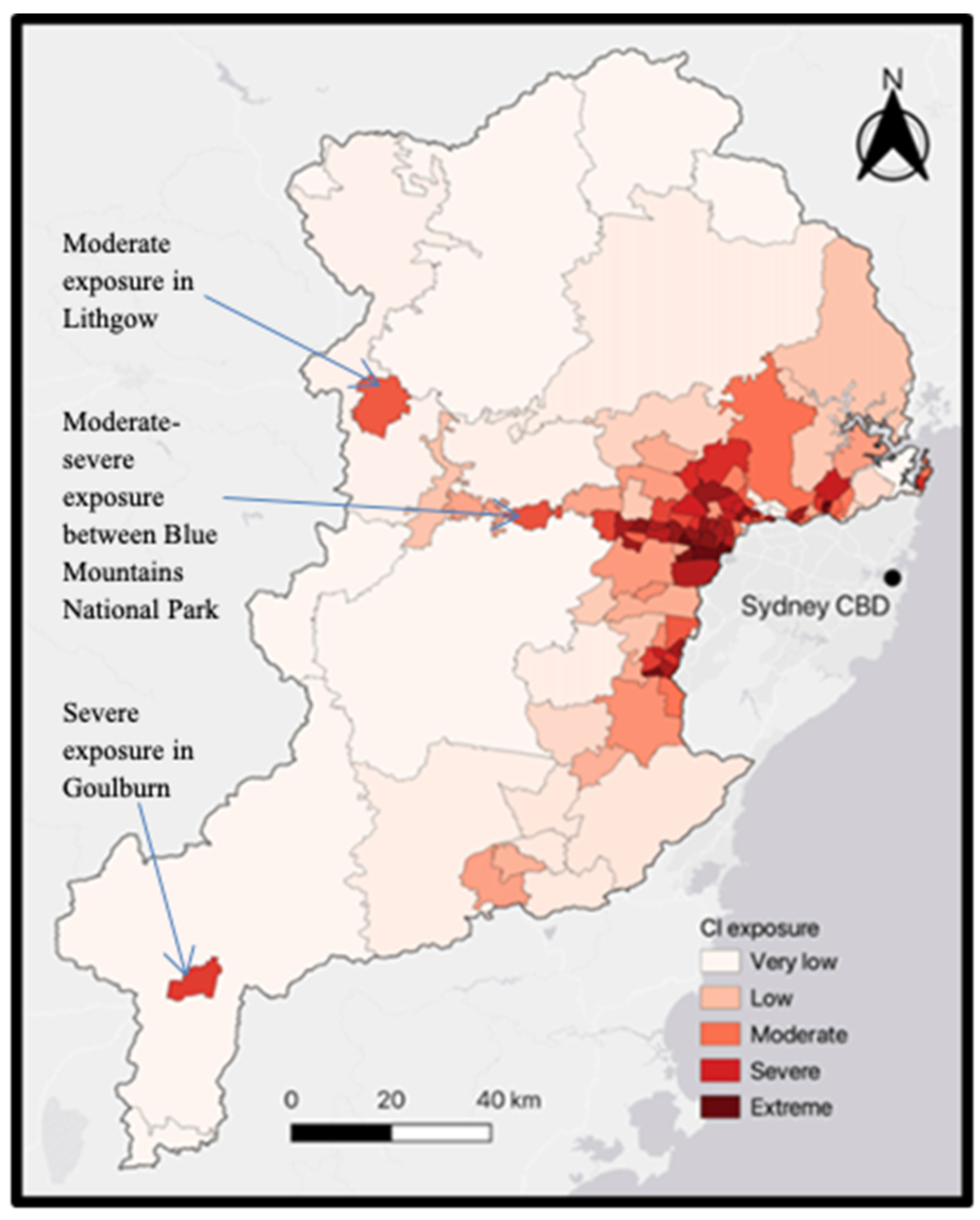
4.3. Critical Infrastructure Exposure

4.3.1. Critical Infrastructure Exposure Patterns

Critical infrastructure (CI) exposure results from this study are particularly important to consider because CI distribution is not dependent on urbanisation alone (urbanisation being the key driver of population density and land use type indicator trends, as outlined). For example, a power station may be located in a less urbanised SA2 because this allows optimal power generation and transmission throughout the HNC.

The obtained results revealed that CI exposure is extreme for SA2s on or near the floodplain of the HNC. This is an urbanised area which would therefore house CI such as hospitals or police stations to meet the needs of the community. However, it is important to note that the SA2s on or near the floodplain are smaller in size. This may have increased final CI density scores, because these are calculated by dividing by land area. Yet, in a similar manner to the population density indicator, the CI indicator was presented as density (rather than absolute values) to standardise between differently sized SA2s in the catchment. This was especially important for this indicator because CI distribution does not necessarily follow expected urbanisation trends, as outlined above.

As per a map of CI flood exposure in the HNC, SA2s surrounding the catchment’s floodplain presented moderate or severe CI exposure, indicating that the amount of CI progressively decreases away from the urbanised Greater Western Sydney region. However, two exceptions existed in the Lithgow and Goulburn SA2s which are far from Greater Western Sydney (see Figure 4). These SA2s presented moderate and severe CI exposure, respectively. Sub-indicator CI exposure trends can be referred to in order to understand these two outliers as well as overall CI distribution patterns (see Figure 6 for details).

A map of CI in the HNC (Figure 6) demonstrates that Lithgow (annotated) has eight CIs within or running through it: one SES office, one police station, one hospital, three broadcast transmission towers, as well as roads and electricity transmission lines. This is a relatively high amount of CI relative to other SA2s outside of the catchment’s floodplain. Furthermore, Goulburn (annotated) has ten: two SES offices, one police station, three hospitals, three broadcast transmission towers, one power substation, as well as roads and some electricity transmission lines. This further reinforces the finding that Goulburn represents what appears to be the most flood-exposed SA2 outside of Greater Western Sydney.

Outside of these areas, SA2s in the HN catchment presented very low or low CI exposure. This indicates that these SA2s are less urbanised and have fewer CIs which contribute to the catchment’s transport network (e.g., roads), communication network (e.g., broadcast transmission towers), or energy grid (e.g., electricity transmission lines, power stations, or power substations). Likewise, it also indicates that these SA2s do not house as many strategically placed CIs which contributes to overall service and utility networks (e.g., power stations connecting to the catchment’s overall energy grid). It can be expected that this aligns strongly with those areas which are sparsely populated. Ultimately, this is an insightful observation that contributes to CI exposure trends throughout the catchment.

4.3.2. Critical Infrastructure Density Indicator Analysis

The fuzzy midpoint and spread used to standardise CI density data were 0.2 and 2, respectively. Such a low fuzzy midpoint may have resulted in some information being lost in the final CI density map, as most values were weighted more highly. However, this approach was again sufficient for this proof-of-concept as it did not produce noticeable or statistically different outliers.

The correlation coefficient for the CI density indicator was 0.67 (statistically significant, p < 0.0001); this intermediate value indicated that CI density was more spatially similar to the final flood exposure index map than land use type, but less than population density. In a similar manner to population density, a higher correlation coefficient value of 0.67 is expected as an easy-to-conceptualise correlation exists between CI density and flood exposure where higher CI density equates to higher flood exposure.

Unlike the other two flood exposure indicators, the CI density methodology used for this study was novel as earlier studies tend to be more limited in their inclusion of CI. It should be noted that this methodology could be replicated for flood exposure assessment and mapping in other flood-prone areas of Australia to produce inland CI exposure results for an index-based FRA. Future work for this indicator also exists in that reclassification and value assigning can be employed to CIs for the HNC, as done for the land use type indicator. Making use of this methodology may produce a more accurate analysis than assuming all CIs in the catchment are flood-exposed to the same extent.

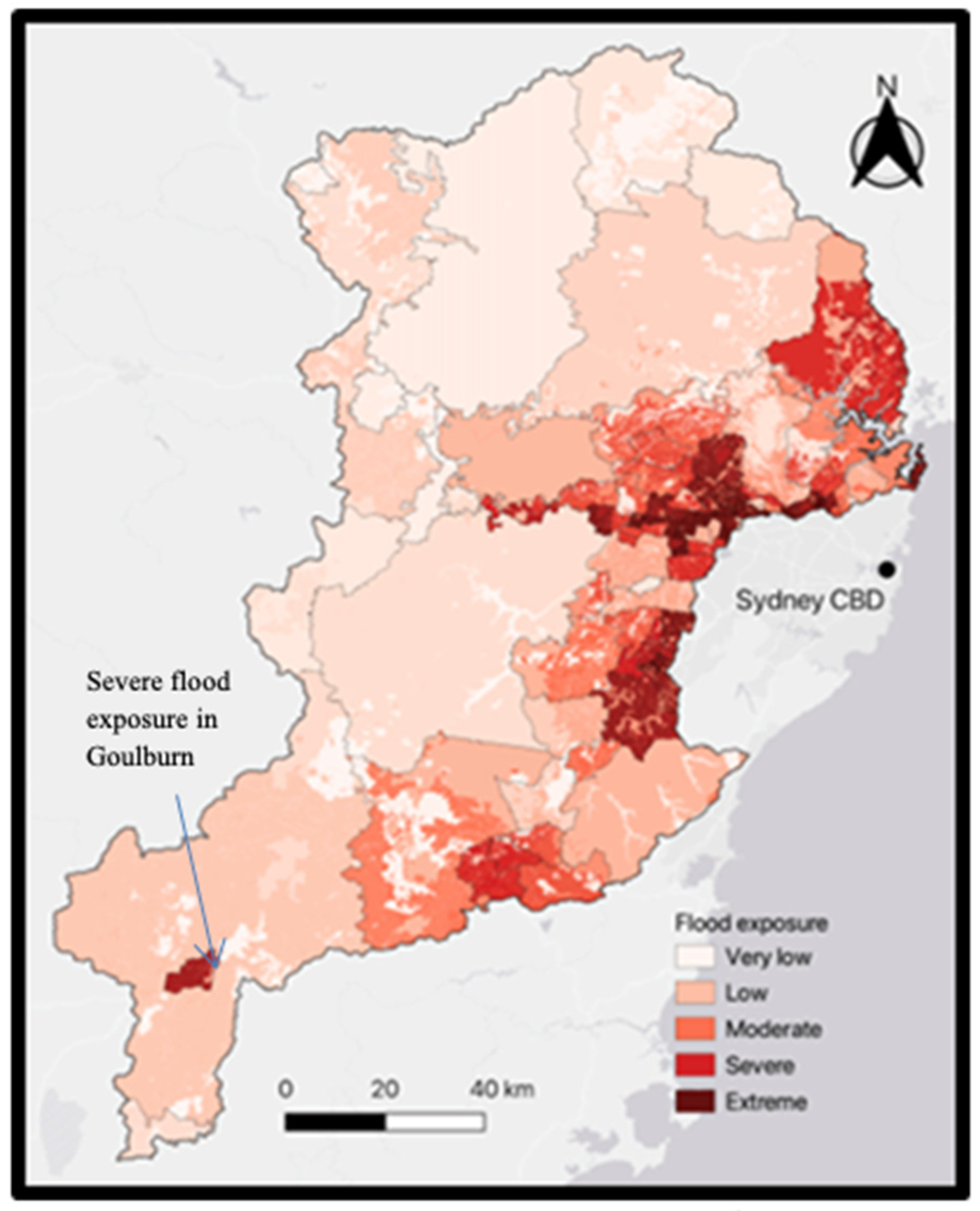
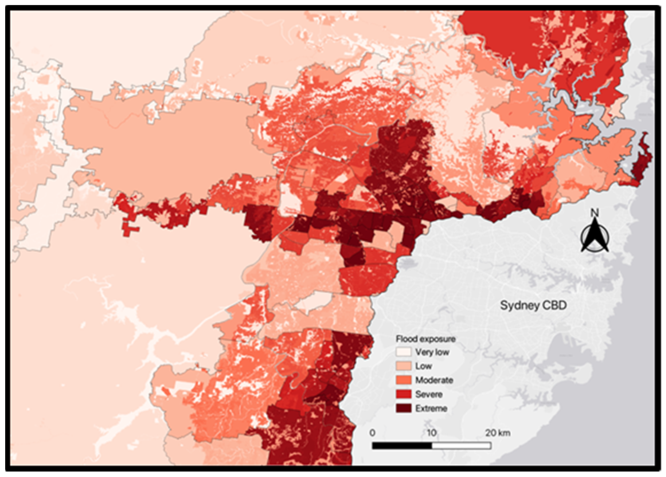
4.4. Flood Exposure Index

The final FEI was derived based on the cumulative inputs of population density, land use type, and critical infrastructure density with their respective distributions. The FEI map revealed two main insights. First, flood exposure increases from very low to extreme levels with increasing proximity to the floodplain within Greater Western Sydney of the HNC (see Figure A2, Appendix H, for smaller SA2s in this area). This is consistent with specific indicator trends mentioned prior, in which more urban growth results in higher flood exposure. Second, outside of Greater Western Sydney, Goulburn (annotated in Figure 5) presented severe flood exposure. This is due to Goulburn’s moderate, extreme, and severe population, land use, and CI exposure, respectively. As mentioned, this is primarily a product of Goulburn’s extent of urbanisation and historic origins.

Importantly, having performed correlation analysis, all correlation coefficient values were positive with flood exposure. The three values were also reasonably close to one another in range, suggesting that they were spatially similar in relation to the FEI. This is desirable for a flood exposure analysis. This is because flood-exposed elements (and so indicators) tend to be more static than dynamic in a given study area—that is, flood-exposed elements (e.g., the amount of hospitals) will not change significantly over time, at least to the extent that flood hazard does, for example. For flood hazard, natural hazards and antecedent conditions can vary significantly on shorter temporal scales, making this risk subcomponent more dynamic. It should also be noted that while these correlation coefficient values are representative of this HNC study area, other flood-prone areas may produce different values to reveal different insights—even with identical or similar flood exposure indicators.

The FEI map can assist local authorities and institutions as well as agencies in all levels of government in identifying priority SA2s in the HNC.

Table 3. SA2s in the Hawkesbury-Nepean Catchment which are severely and extremely exposed to inland flood.

SA2	Flood Exposure Score (Mean)	Flood Exposure Risk Class
Wahroonga (West)—Waitara	0.990	Extreme
Acacia Gardens	0.964	Severe
Glendenning—Dean Park	0.963	Severe
Cambridge Park	0.947	Severe
Goulburn	0.851	Severe

presents a list of severely and extremely exposed SA2s, based on the methodology and scope of this study. These SA2s presented the highest FEI scores, averaged throughout each SA2. Although Goulburn presented a lower score, it is included because it was the only SA2 which was found to be particularly flood-exposed outside of Greater Western Sydney.

These findings may encourage certain resources to be allocated to severely or extremely flood-exposed SA2s, with more robust evidence-based flood risk management approaches to be implemented in such SA2s in the short- and long-term (such as early warning systems), and tailored government funding. By providing an overall snapshot of the catchment’s flood exposure at SA2, the FEI map can also be used to inform key decision making. Importantly, it can contribute to discussion outside of flood risk; for example, by aiding in climate change adaptation strategies or more general multi-hazard analyses which consider the interrelated and compounding effects between natural hazards over time.

This study ultimately contributes to improving Australian FRAs in this space by suggesting a novel catchment-wide and index-based methodology on flood exposure, rather than solely flood hazard, which is typical of most flood management guidelines for councils in Australia. As mentioned, such flood management guidelines rarely assess at a catchment level, nor do they utilise indices or explore less-characterised but equally important flood risk subcomponents of flood exposure and vulnerability. The findings from this study, which align with expected trends and are in turn bolstered by future validity analysis, begin to suggest that this research substantially improves upon the FRA framework and assumes a strong and successful methodology.

Future work in this space can focus on embellishing the FEI map so that it is more specific to an inland flood context as well as the characteristics of the HNC. For example, future research could provide strong justification behind the flood exposure values assigned to reclassified land use types for the land use type indicator. Additionally, a validity analysis should also be conducted for the FEI to ensure that findings are scientifically accurate. Doing so would also bring strong merit to any subjectivity introduced by this study’s methodology. One such method which can be considered for this is the Receiver Operating Characteristic curve analysis, which is well-established in the literature (e.g., [38,39]). Finally, this study’s methodology can be tested for other study areas outside of the HNC to ensure it is robust and replicable. This would enhance the methodology by producing comparable findings. This study’s methodology can also be applied to that of flood hazard and vulnerability, so that flood risk is successfully characterised for the HNC based on the aforementioned risk triangle framework. For example, for flood hazard, maps derived from remote-sensing satellites can be employed as points of reference when comparing hydrological modelling and index-based approaches commonly seen in Australian FRAs (e.g., [40,41]).

5. Conclusions

The aim of this study was to develop and map a flood exposure index for NSW’s Hawkesbury-Nepean Catchment, based on a set of key and easily sourced indicators. The indicators chosen were population density, land use type, and critical infrastructure density. This research can in turn be bolstered by flood hazard and vulnerability indices for the catchment within the context of overall flood risk.

It was found that flood exposure is higher on or near the catchment’s floodplain rivers, alongside the Hawkesbury and Nepean Rivers and related tributaries. This is due to urban development around the floodplain, which in turn results in higher population, land, and critical infrastructure exposure. Goulburn also presented extreme flood exposure, despite being a great distance from the floodplain to the east of the catchment. This is due to its historic origins as NSW’s first inland town, which has provided the opportunity for socioeconomic development and thereby higher flood exposure.

This study is a valuable contribution to the discussion of flood management in Australia and abroad. The strongly correlated indicators of population density, land use type, and critical infrastructure density are suitable proxies in describing the flood-exposed landscape of NSW’s Hawkesbury-Nepean Catchment. Insights from this proof-of-concept can also assist flood mitigation and adaptation in other flood-prone areas outside of the study area; this is bolstered by the openly accessible nature of an index-based methodology. Ultimately, this novel research can help relevant stakeholders to better understand flood risk management for disaster risk reduction. In an increasingly flood-prone landscape in the presence of anthropogenic climate change, the replicable and scalable Flood Risk Assessment scoped by this research will be key to meaningful and proactive action on flood mitigation and adaptation. It is recommended that the methodology used for this study is considered as a potential framework for further index-based flood assessment approaches.

References

1. Australian Bureau of Meteorology (BoM). Understanding Floods; Australian Government Bureau of Meteorology: Melbourne, Australia, 2022. Available online: http://www.bom.gov.au/australia/flood/knowledge-centre/understanding.shtml (accessed on 21 May 2022).
2. FitzGerald, G.; Du, W.; Jamal, A.; Clark, M.; Hou, X.-Y. Flood Fatalities in Contemporary Australia (1997–2008). Emerg. Med. Australas. 2010, 22, 180–186. [Google Scholar] [CrossRef] [PubMed]
3. Bates, P.D.; Quinn, N.; Sampson, C.; Smith, A.; Wing, O.; Sosa, J.; Savage, J.; Olcese, G.; Neal, J.; Schumann, G.; et al. Combined Modeling of US Fluvial, Pluvial, and Coastal Flood Hazard Under Current and Future Climates. Water Resour. Res. 2021, 57, e2020WR028673. [Google Scholar] [CrossRef]
4. Pittock, B.; Abbs, D.; Suppiah, R.; Jones, R. Climatic Background to Past and Future Floods in Australia. In Advances in Ecological Research; Floods in an Arid Continent; Academic Press: Cambridge, MA, USA, 2006; Volume 39, pp. 13–39. [Google Scholar] [CrossRef]
5. Intergovernmental Panel on Climate Change (IPCC). Summary for policymakers. In Climate Change 2022: Impacts, Adaptation and Vulnerability. Contribution of Working Group II to the Sixth Assessment Report of the Intergovernmental Panel on Climate Change; Cambridge University Press: Cambridge, UK, 2022. [Google Scholar]
6. UN Expert Group. Natural Disasters and Vulnerability Analysis: Report of Expert Group Meeting, 9–12 July 1979; Office of the UN Disaster Relief Coordinator: Geneva, Switzerland, 1980. [Google Scholar]
7. Crichton, D.; Ingleton, J. (Eds.) The Risk Triangle; Natural Disaster Management: London, UK, 1999; pp. 102–103. Available online: https://www.ilankelman.org/crichton/1999risktriangle.pdf (accessed on 12 May 2022).
8. Australian Institute for Disaster Resilience (AIDR). Flood Hazard Guideline 7-3; Australian Institute for Disaster Resilience: Melbourne, Vic, Australia, 2017; Available online: https://knowledge.aidr.org.au/media/3518/adr-guideline-7-3.pdf (accessed on 12 May 2021).
9. de Brito, M.M.; Evers, M. Multi-Criteria Decision-Making for Flood Risk Management: A Survey of the Current State of the Art. Nat. Hazards Earth Syst. Sci. 2016, 16, 1019–1033. [Google Scholar] [CrossRef] [Green Version]
10. Espada Jr., R.; Apan, A.; McDougall, K. Understanding the January 2011 Queensland Flood: The Role of Geographic Interdependency in Flood Risk Assessment for Urban Community. In Proceedings of the Australian and New Zealand Disaster and Emergency Management Conference (ANZDMC 2013), Brisbane, Qld, Australia, 28–30 May 2013; AST Management Pty Ltd.: Gold Coast, Australia, 2013; pp. 68–88. [Google Scholar]
11. Rashetnia, S.; Jahanbani, H. Flood Vulnerability Assessment Using a Fuzzy Rule-Based Index in Melbourne, Australia. Sustain. Water Resour. Manag. 2021, 7, 13. [Google Scholar] [CrossRef]
12. Ologunorisa, T.; Abawua, M. Flood Risk Assessment: A Review. J. Appl. Sci. Environ. Manag. 2005, 9, 57–63. [Google Scholar] [CrossRef]
13. Rafiei-Sardooi, E.; Azareh, A.; Choubin, B.; Mosavi, A.H.; Clague, J.J. Evaluating Urban Flood Risk Using Hybrid Method of TOPSIS and Machine Learning. Int. J. Disaster Risk Reduct. 2021, 66, 102614. [Google Scholar] [CrossRef]
14. Kelly, M.; Kuleshov, Y. Flood Hazard Assessment and Mapping: A Case Study from Australia’s Hawkesbury-Nepean Catchment. Sensors 2022, 22, 6251. [Google Scholar] [CrossRef]
15. Schwarz, I.; Kuleshov, Y. 2022: Flood Vulnerability Assessment and Mapping: A Case Study for Australia’s Hawkesbury-Nepean Catchment. Remote Sens. 2022, 14, 4894. [Google Scholar] [CrossRef]
16. Infrastructure NSW. Hawkesbury-Nepean Valley Flood Risk Management Strategy. 2017. Available online: https://www.infrastructure.nsw.gov.au/media/1534/insw_hnvfloodstrategy__1_v2.pdf (accessed on 14 May 2022).
17. Australian Government Infrastructure Australia. Hawkesbury-Nepean Valley Flood Management. 2022. Available online: https://www.infrastructureaustralia.gov.au/map/hawkesbury-nepean-valley-flood-management (accessed on 14 May 2022).
18. Cremen, G.; Galasso, C.; McCloskey, J. Modelling and Quantifying Tomorrow’s Risks from Natural Hazards. Sci. Total Environ. 2022, 817, 152552. [Google Scholar] [CrossRef]
19. Ming, X.; Liang, Q.; Dawson, R.; Xia, X.; Hou, J. A Quantitative Multi-Hazard Risk Assessment Framework for Compound Flooding Considering Hazard Inter-Dependencies and Interactions. J. Hydrol. 2022, 607, 127477. [Google Scholar] [CrossRef]
20. Junger, L.; Hohensinner, S.; Schroll, K.; Wagner, K.; Seher, W. Land Use in Flood-Prone Areas and Its Significance for Flood Risk Management—A Case Study of Alpine Regions in Austria. Land 2022, 11, 392. [Google Scholar] [CrossRef]
21. Ahmed, A.; Hewa, G.; Alrajhi, A. Flood Susceptibility Mapping Using a Geomorphometric Approach in South Australian Basins. Nat. Hazards 2021, 106, 629–653. [Google Scholar] [CrossRef]
22. Membele, G.M.; Naidu, M.; Mutanga, O. Examining Flood Vulnerability Mapping Approaches in Developing Countries: A Scoping Review. Int. J. Disaster Risk Reduct. 2022, 69, 102766. [Google Scholar] [CrossRef]
23. Papathoma-Köhle, M.; Schlögl, M.; Dosser, L.; Roesch, F.; Borga, M.; Erlicher, M.; Keiler, M.; Fuchs, S. Physical Vulnerability to Dynamic Flooding: Vulnerability Curves and Vulnerability Indices. J. Hydrol. 2022, 607, 127501. [Google Scholar] [CrossRef]
24. Pant, R.; Thacker, S.; Hall, J.; Alderson, D.; Barr, S. Critical Infrastructure Impact Assessment Due to Flood Exposure. J. Flood Risk Manag. 2018, 11, 22–23. [Google Scholar] [CrossRef]
25. NSW Government. NSW Critical Infrastructure Resilience Strategy. 2018. Available online: https://www.opengov.nsw.gov.au/publications/19460;jsessionid=8A7CF4082E06B2D165B02408F82BE1A3 (accessed on 14 May 2022).
26. Australian Bureau of Statistics (ABS). Statistical Area Level 2. 2021. Available online: https://www.abs.gov.au/statistics/standards/australian-statistical-geography-standard-asgs-edition-3/jul2021-jun2026/main-structure-and-greater-capital-city-statistical-areas/statistical-area-level-2#:~:text=Statistical%20Areas%20Level%202%20(SA2s,Australia%20without%20gaps%20or%20overlaps (accessed on 14 May 2022).
27. NSW Government. State of the Catchments 2010: Hawkesbury-Nepean Region; Department of Environment, Climate Change and Water: Sydney, NSW, Australia, 2010. [Google Scholar]
28. Doganay, E.; Magaziner, J. Flash Flooding and Green Stormwater Infrastructure in Philadelphia: Areas for Further Improvement. Turk. J. Water Sci. Manag. 2017, 1, 18. [Google Scholar] [CrossRef]
29. Hagos, Y.G.; Andualem, T.G.; Yibeltal, M.; Mengie, M.A. Flood Hazard Assessment and Mapping Using GIS Integrated with Multi-Criteria Decision Analysis in Upper Awash River Basin, Ethiopia. Appl. Water Sci. 2022, 12, 148. [Google Scholar] [CrossRef]
30. Aitkenhead, I.; Kuleshov, Y.; Watkins, A.B.; Bhardwaj, J.; Asghari, A. Assessing Agricultural Drought Management Strategies in the Northern Murray–Darling Basin. Nat. Hazards 2021, 109, 1425–1455. [Google Scholar] [CrossRef]
31. James, A.; Rowley, S.; Davies, A.; Ong, R.; Singh, R. Population Growth and Mobility in Australia: Implications for Housing and Urban Development Policies; Report; Australian Housing and Urban Research Institute: Melbourne, VIC, Australia, 2021. [Google Scholar]
32. Northern Beaches Council. Visit Northern Beaches Council. 2022. Available online: https://www.northernbeaches.nsw.gov.au/things-to-do/visit (accessed on 15 May 2022).
33. Tomar, P.; Singh, S.K.; Kanga, S.; Meraj, G.; Kranjčić, N.; Đurin, B.; Pattanaik, A. GIS-Based Urban Flood Risk Assessment and Management—A Case Study of Delhi National Capital Territory (NCT), India. Sustainability 2021, 13, 12850. [Google Scholar] [CrossRef]
34. Feng, B.; Zhang, Y.; Bourke, R. Urbanization Impacts on Flood Risks Based on Urban Growth Data and Coupled Flood Models. Nat. Hazards 2021, 106, 613–627. [Google Scholar] [CrossRef]
35. Amadio, M.; Mysiak, J.; Marzi, S. Mapping Socioeconomic Exposure for Flood Risk Assessment in Italy. Risk Anal. 2019, 39, 829–845. [Google Scholar] [CrossRef]
36. Maheshwari, B.; Plunkett, M.; Singh, P. Farmers’ Perceptions about Irrigation Scheduling in the Hawkesbury-Nepean Catchment; Sydney, NSW, Australia. 2003. Available online: http://www.regional.org.au/au/apen/2003/refereed/113maheshwari.htm (accessed on 14 May 2022).