Abstract
Soil erosion caused by intense rainfall events is one of the major problems affecting agricultural and forest ecosystems. The Universal Soil Loss Equation (USLE) is probably the most adopted approach for rainfall erosivity estimation, but in order to be properly employed it needs high resolution rainfall data which are often unavailable. In this case, empirical formulas, employing aggregated rainfall data, are commonly used. In this work, we select 12 empirical formulas for the estimation of the USLE rainfall erosivity in order to assess their reliability. Moreover, we used a Stochastic Rainfall Generator (SRG) to simulate a long and high-resolution rainfall time series with the aim of assessing its application to rainfall erosivity estimations. From the analysis, performed in the Rieti province of Central Italy, we identified three equations which seem to provide better results. Moreover, the use of the selected SRG seems promising and it could help in solving the problem of hydrological data scarcity and consequently guarantee major accuracy in soil erosion estimation.
1. Introduction
Soil erosion caused by intense rainfall events is recognized as one of the major problems affecting agricultural and forest ecosystems [1]. Heavy rainfall can indeed provoke phenomena such as shallow landslides, soil loss, pollution of water bodies and can decrease crop productivity [2]. Studies on soil erosion, aiming to select solutions for limiting the soil loss, are hence crucial for conserving and protecting the environment [3]. Since the first decades of the last century, they have increased in number and variety and, in recent years, the soil loss due to rainfall erosivity has been systematically analyzed [4].
Many mathematical models of soil erosion have been developed by the scientific community. One pivotal contribution can be represented by the studies of Wischmeier and Smith [5,6], which gave birth to the worldwide known Universal Soil Loss Equation (USLE), later rearranged in the revised USLE (RUSLE) [7,8]. USLE and its modifications are probably the most adopted approaches to estimate soil erosion.
The soil erosion caused by heavy rainfall occurs with the detachment of soil particles due to the impact of the raindrops and the subsequent downslope transport of the detached material [9]. This is a complex phenomenon that is a combination of different rainfall characteristics, such as intensity and duration, mass and diameter of rainfall drops, plus other factors depending on soil properties, e.g., topographic characteristics, and agroforestry practices.
Concerning rainfall erosivity, USLE expresses the impact of rainfall on soil loss using a rainfall erosivity factor, R. In the original formulation, the R-factor has been defined as the summation of the total storm energy (E) of an erosive rainfall event multiplied by the corresponding maximum rainfall intensity calculated at 30 min resolution (I30) within a certain period, for instance, one year [10]. The original method requires the use of continuous long-term and high-resolution rainfall data for its proper application, but unfortunately this kind of information is usually difficult to obtain due to the commonly reduced number and unequal spatial distribution of rain gauge stations where pluviographic data are available [11]. A second drawback is represented by the common lack of long-term high-resolution rainfall data [12], leading to a low availability of accurate R-factor values for many countries [13].
In order to overcome such drawbacks, the original R-factor calculation is often replaced by the use of empirical formulas, where simple pluviometric information, such as annual, monthly or daily rainfall amounts are present [14,15,16]. However, empirical equations should be applied with caution, because they are usually based on regressions among locally measured data and cannot be applied in larger areas [17]. Moreover, such formulas could not capture the high rainfall intensities, which usually occur at very short time scales and have a significant influence on rainfall erosivity [12]. Indeed, hydrological estimation measures in small and ungauged basins represent a challenging and open research topic for hydrologists [18].
Consequently, in this context of uncertainty, the use of Stochastic Rainfall Generators (SRG) appears helpful for a more in-depth analysis of rainfall-related processes, mainly for obtaining long rainfall time series which are representative of rainfall fields at hydrological spatial and temporal scales. The use of a SRG for rainfall-related processes analyses has been successfully tested in a wide variety of climatic conditions [19,20,21,22,23]. However, some works [24,25] showed that R-factors calculated using synthetic rainfall series often need to be calibrated due to systematic discrepancies of real R-factor values. Thus, we believe that the use of SRG should be more deeply investigated with the aim to assess their application to rainfall erosivity estimation.
Considering all the aforementioned, the aims of the manuscript are as follows:
- To apply to a selected case study corresponding to the Rieti province, in Central Italy, a selection of empirical formulas for the estimation of the rainfall erosivity using the USLE approach, in order to assess the uncertainty in the rainfall erosivity estimation due to the specific empirical formula. The most appropriate empirical formulas will be assessed using a proposed index of reliability. It is noteworthy that the Rieti province, characterized by a mountainous environment and a rainy climate, is lacking an official R-factor map and an official rainfall erosivity estimation.
- To apply, in one rain gauge station of Rieti province, a new and recently developed SRG, parsimonious in terms of input parameters. The application of the SRG allows the synthetic generation of a high-resolution time series that can be used for estimating the rainfall erosivity, employing the same empirical formulas of previous point 1), or using the original USLE formulation. Such application will allow assessment if the proposed SRG can be a suitable alternative for the estimation of soil erosion in case of rainfall data scarcity.
It is important to underline that the novelty of this work is represented by the use of the proposed SRG for rainfall erosivity estimation, and by the introduction of the index of reliability that gives the possibility to choose the most appropriate formula for each selected case study. Moreover, the definition of rainfall erosivity maps for the province of Rieti can be very important for land panning and management. Knowing the areas where a great R-factor value is supposed to be can be helpful in localizing areas prone to soil erosion and hydro-geological risk.
The present manuscript is organized as follows: in Section 2, materials and methods are described. In particular, the paragraph describes the selected case study, reports the investigated formulas, and illustrates the proposed SRG. In Section 3, results are presented and discussed, while in Section 4 the conclusions are reported.
2. Materials and Methods
2.1. Study Area
The selected study area, shown in Figure 1, is the Rieti province, located in the Lazio region of Central Italy. The study area has an extension equal to 2749 km² and it includes 73 municipalities with a total number of inhabitants greater than 155,000. The landscape, vegetation and climate are vary extremely, for instance the elevations range from 25 to almost 2500 m a.s.l.. Typical alluvial valleys, such as the Tiber River and Velino River valleys are present; however, high mountains, such as Terminillo (2217 m) and Monte Navegna (1508 m), that are part of the Apennines, are also visible.
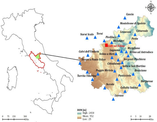
Figure 1.
Study area localization. Left: Italy (grey border), Lazio region (red border), Rieti province (filled green). Right: Rieti province digital elevation model (DEM) with rain gauge stations (blue triangles) and Colli sul Velino rain gauge station (red square).
Climate and Vegetation of the Study Area
The Rieti province belongs to the Italian temperate eco-regional division [26]. This division embraces the northern and inner part of the Italian peninsula, including the main orographic chains of the Alps and the Apennines. It is characterized by a temperate climate, with annual medium temperatures above 5 °C and 4–8 months with medium temperatures below 10 °C. The mountain sectors above 1500 m present a prolonged winter season. Annual thermal excursion is marked. The minimum temperatures of the coldest month (January) are always below 3 °C, not excluding the possibility of frosts, while the maximum temperatures exceed 30 °C in the warmest months (July and August) at hilly elevations. Annual precipitation ranges almost everywhere from 800 mm up to over 2000 mm, so the pluviometric regime can be considered as Continental (with a winter minimum) or Apenninic (with a summer minimum and two maxima in autumn and spring). In the summer season, the aridity period is generally not remarkable and, in any case, shorter than 2 months.
With specific reference to the Rieti province, the annual precipitation ranges from 1200 to 1600 mm, with October, November, and December being the rainiest months [27]. Rainfall has two maxima, the main one in autumn and the second in late spring [28]. The summer aridity period is limited to the months of July and August [27]. Figure 2 confirms the descripted monthly trend. The winter season generally lasts 140 days, covering part of spring [28]. Snow falls generally on hills and mountains, rarely on the valley where it is instead possible to have some foggy days, especially during spring and autumn.
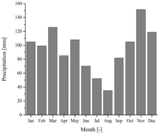
Figure 2.
Observed precipitation data in Rieti province from 2008 to 2018.
Regarding the rainfall data, all the rain gauge stations located inside the selected case study area, and in the immediate external proximity, have been identified from the regional hydrographic offices. Rain gauge stations used in the present work have been selected with the compromise of having both a great number of stations, in order to accurately describe the spatial rainfall distribution, and an adequate number of observed years of rainfall data, in order to accurately characterize the temporal rainfall distribution. In doing so, we selected 30 rain gauge stations, shown in Figure 1, characterized by a continuous daily rainfall data availability ranging from 2008 to 2018, for a total of 11 years. Although we are aware that 11 years is not a great number for an accurate statistical rainfall estimation, it is noteworthy that the data scarcity is a common problem for researchers and practitioners, leading often to analyze a limited number of rainfall data for similar applications. Some examples can be found in Diodato and Bellocchi [4] and in Porto [29], which analyzed stations with only 4 or 5 years of data for a rainfall erosivity estimation employing the USLE formulation.
The majority (19) of the rain gauge stations here selected are located in Lazio region, Rieti province. Five rain gauge stations are located in Lazio region, Roma province, and the remaining six rain gauge stations are located in Umbria region, in the provinces of Perugia and Terni. From the retrieved daily data, it was possible to calculate the USLE R-factor according to the methodologies presented in the following paragraphs.
The complex landscape of the Rieti province with river valleys characterized by the presence of different lakes (the largest lakes are represented by the Ripasottile Lake, located in the Rieti Plain and about 2 km long, and the Salto Lake in the Salto Valley, about 10 km long, and the surrounding Appenninic chains (Monti Reatini, mountains of Salto and Turano valleys, Monti Sabini)) lead to a great variability in habitats and vegetation patterns. River and lake vegetation in the valleys cohabit with extensive crops, mainly maize and cereal cultivation [30], and olive trees on hills. With specific reference to the forest vegetation, it appears similar to a mosaic due to the local variations in terms of altitude, rainfall, temperature and sun exposure. The huge variation in altitude has influenced the distribution of agricultural, silvicultural, and breeding activities during time, and indirectly that of forests.
In relation to the altitude, it is possible to identify at least 15 different forest types. Among them, the most important are beech forests (Fagus sylvatica), chestnuts forests (Castanea sativa), deciduous oak forests (Quercus cerris, Q. robur and Q. pu-bescens) and evergreen oak forests (Quercus ilex).
2.2. USLE R-Factor Original Calculation
Wischmeier [31] was the first to introduce a rainfall erosion index for the soil erosion calculation, paving the way for the USLE - Universal Soil-Loss Equation [5,6]. USLE is one of the most used empirical equations to calculate the theoretical soil erosion in a determinate area, mainly because of its easy employment in terms of calculation and reduced requirement of input data [32]. Since its development, this equation was subject to different modifications and improvements, mainly made to allow its use in GIS environments. It is for this reason that the RUSLE (Revised Universal Soil Loss Equation) [7] was developed. The original USLE equation is expressed as follows:
where A is the annual soil erosion (t * ha−1 * year−1), R is the rainfall erosivity factor (MJ * mm * ha−1 * h−1 * year−1), K is the soil erodibility factor (t * ha−1 * [MJ * (ha * mm)−1 * ha−1]* year−1), LS is the product between length (L) and slope (S) factors (dimensionless), C is the soil coverage and management factor (dimensionless) and P is the support practice factor (dimensionless).
A = R × K × LS × C × P
The rainfall erosivity factor represents the erosivity power that rainfall has on the soil in a determinate area. In its first formulation, the R-factor was defined as the summation of the total storm energy (E) of an erosive rainfall event multiplied by the corresponding rainfall maximum intensity over a time span of 30 min (I30) within a certain time period, for instance one year [10]. It was expressed as follows:
where: EI30 = E × I30; E = 916 + 331*log10(I), with I being the rainfall intensity (in* h−1); (EI30)i is related to storm i-th and j is the total number of storms in an N-year period. It is noteworthy that units of Equation (2) are imperial (R is expressed in 100 foot-ton * in * acre−1 * h−1 * year−1) and that results should be multiplied by 17.02 to convert in metric units (R expressed in MJ * mm * ha−1 * h−1 * year−1).
As it can be noted from Equation (2), the USLE R-factor calculation using the original formulation is possible only if high resolution (at 30 min) rainfall data are available. Due to data scarcity and inaccuracy of old rain gauge stations, many authors elaborated alternative approaches for R-factor estimation, proposing different empirical formulas that are reported in the following paragraph.
2.3. Alternative Approaches for USLE R-Factor Calculation
When high resolution rainfall data are not available, alternative approaches can be used for calculating rainfall erosivity. Almost all these approaches make use of monthly and yearly cumulative rainfall data, or the Modified Fournier Index [33,34]. From an extensive literature analysis, we identified 12 empirical formulas, listed in Table 1, that have been often applied in Mediterranean countries and in semiarid areas.

Table 1.
Rainfall erosivity equations used in this work.
The use of the 12 investigated empirical formulas allowed the calculation of rainfall erosivity for all the selected rain gauge stations using the daily data recorded in the period 2008–2018, assessing the uncertainty in the rainfall erosivity estimation due to the specific applied formulation.
From the values of rainfall erosivity estimated at the rain gauge stations, it was possible to create rainfall erosivity GIS maps, using the software ArcMap 10.6 and a Kriging interpolation. This allowed us to create rainfall erosivity maps of the province of Rieti for all the empirical analyzed formulas.
2.4. The Stochastic Rainfall Generator (SRG)
Many works (see [43], for a list of references) highlighted the capacity of a specific class of SRGs, i.e., the Poisson cluster models, to satisfactorily reproduce observed summary statistics, such as mean, variance, skewness, proportion of dry/wet periods, and k-lag autocorrelation values, of the continuous rainfall process at several fine time scales. Poisson cluster models mainly comprise of Neyman–Scott and Bartlett–Lewis families, which perform equally well [43]. In this context, the most adopted shape for a rain cell in literature, i.e., the rectangular one, is considered in this work and then the Neyman–Scott Rectangular Pulses (NSRP, [43]) are adopted.
The NSRP model is based on the following assumptions from (a) to (d) (see Figure 3): (a) the inter-arrival time between the origins of two consecutive storms is assumed as an independent and identically distributed random variable, and it follows an exponential distribution; (b) each storm includes a number of rain cells (also indicated as bursts or pulses). Such a number is set as geometrically distributed, with the goal of having at least one burst for each storm. Each burst origin occurs, from the associated storm origin, after a waiting time, which is assumed as an exponentially distributed variable; (c) each burst has a rectangular shape, with an intensity and a duration that are both considered as exponential distributed; and (d) the total precipitation intensity at time t is then calculated as the sum of the intensities that are related to the active bursts at time t, starting from rainfall intensities, the aggregated process, i.e., the rainfall height cumulated at the desired temporal resolution, can be calculated.
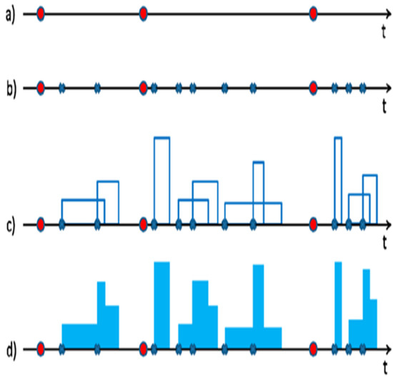
Figure 3.
Representation of the (NSRP) stochastic process for at-site rainfall modeling (from [43]): (a) occurrences of storms; (b) for each storm, determination of the number of pulses and their temporal occurrences; (c) estimation of intensity and duration for all the pulses; (d) calculus of total intensity at time t.
The model has a set of parameters that are usually calibrated by minimizing an objective function, which is defined as the sum of residuals between the considered statistical properties of the observed data at chosen resolutions and their theoretical expressions. The statistical properties are typically referred to as a high-resolution continuous time series. However, continuous high-resolution data sets are very short or absent in many locations, with respect to Annual Maximum Rainfall (AMR) with different durations that usually are available with an adequate sample size. For this reason, the possibility to calibrate the model using only AMR data [43,44,45] and basic statistics, such as cumulate values for monthly or annual rainfall, has been adopted here. Such choice allows for a better reconstruction of extreme events, which are of main interest in many hydrological studies, for instance in the case of soil erosion caused by intense rainfall events.
Moreover, De Luca et al. [46,47] proposed a parsimonious modelling of seasonality, which was adopted in this work. The goal is to avoid an over parameterization by using monthly or seasonal parameter sets. In detail, due to the fact that the information regarding the seasonality of the rainfall process during the year is lost with the use of an AMR series, a simple goniometric series can be defined for any summary statistic of interest for the model.
In conclusion, the NSRP model is calibrated here by selecting the set of parameters, which optimizes the reproduction of mean values for hourly/multi-hourly AMR, plus the cumulative values for the annual rainfall. Then, validation is carried out by comparing the sample and theoretical Amount-Duration-Frequency (ADF) curves for hourly and multi-hourly rainfall heights.
The described NRSP model has been applied in one of the previously described rain gauge stations, i.e., Colli sul Velino station (see Figure 1). The choice of such a station is due to the availability of both daily rainfall data and AMR rainfall data for different durations, a circumstance that allows the comparison of modeled and observed rainfall data not only for daily durations, but also for sub-daily durations. The comparison will allow an assessment if the proposed SRG can be a suitable alternative for the estimation of rainfall erosivity.
3. Results and Discussion
3.1. Analysis of Rainfall Erosivity in Rieti Province
Rainfall erosivity has been calculated using 12 empirical formulas (Table 1). After having calculated, for every single year the rainfall erosivity values, the mean, maximum and minimum values for each equation were examined for the whole period. The average rainfall erosivity values have been reported in Figure 4, where rain gauge stations are numbered in order of decreasing observed yearly cumulative rainfall value.
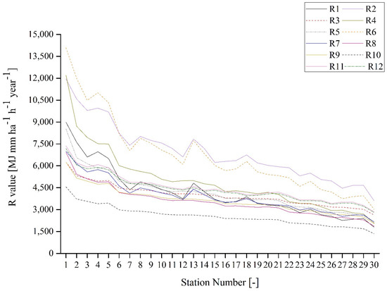
Figure 4.
Average rainfall erosivity values obtained with the selected 12 formulas for each Rain gauge station. The stations were numbered in order of decreasing observed yearly cumulative rainfall value.
It is interesting to note the spatial geomorphological characteristics of the study area. In Figure 5, the rainfall erosivity maps obtained with the 12 investigated empirical formulas are shown. As it is possible to see, even if the maximum rainfall erosivity values vary a lot between all the maps, these are always located in the Monte Terminillo area, where the highest mountains of the province are located. It is also interesting to note that other high mountains are located in the South East part of the Rieti province, but not so high rainfall erosivity values have been obtained for such stations.
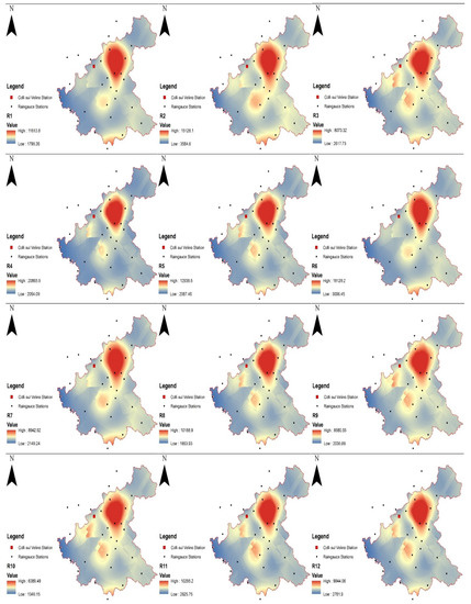
Figure 5.
Rainfall erosivity maps created using the 12 equations. All the values are expressed in MJ * mm * ha−1 * h−1 * year−1.
Finally, Figure 6 shows the minimum, average, and maximum rainfall erosivity values for all the formulas investigated, considering all years from 2008 to 2018. As it possible to see, there are not big differences between the average values of all the formulas. Only R2, R6, and R10 are quite different, with R2 and R6 having a higher value than the mean, and R10 a lower value than the mean. Concerning the minimum rainfall erosivity values, they too are similar, and the differences are negligible.
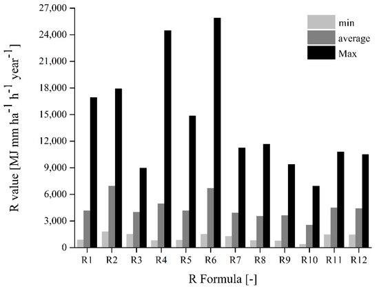
Figure 6.
Minimum, average, and maximum rainfall erosivity values obtained with the 12 selected formulas.
Even if the average and minimum values are similar, we can observe strong differences between all the formulas in the maximum rainfall erosivity values. Here the difference of the values can vary from about 8000 MJ * mm * ha−1 * h−1 * year−1, that is the lowest maximum value (R10), to more than 24,000 MJ * mm * ha−1 * h−1 * year−1 for R4 and R6 formulas.
The rain gauge station that generated the maximum rainfall erosivity values is the Monte Terminillo station (Station number 18 in Figure 4), in the year 2010. In the year 2010, it is possible to see that 14 of the rain gauge stations produced their rainfall erosivity maximum values.
The rainfall erosivity equations that generated the maximum values are R4 and R6, both coming from Renard and Freimund’s research [37]. The first one utilizes the annual mean precipitation, the second one the Modified Fournier Index (MFI), and both are exponential equations. It is interesting to note that R5, that comes from the same research, does not have such a high maximum rainfall erosivity value. Indeed, the maximum value for this equation is almost 15,000 MJ * mm * ha−1 * h−1 * year−1, while R4 and R6 present a 25,000 MJ * mm * ha−1 * h−1 * year−1 value.
From the aforementioned analysis, it is not possible to individuate a reference equation to estimate the rainfall erosivity, probably because too few rainfall data are available. In fact, the sample of data at our disposal is not "hydrologically" significant.
In order to overcome the scarce availability of rainfall data and to individuate a reference equation for rainfall erosivity, an additional analysis has been conducted, using 50 years of synthetic rainfall time series generated for Colle sul Velino rain gauge station (Station number 13 in Figure 4). The rain gauge station choice is based on the considerations seen in Figure 5, where it appears evident that Colli sul Velino station could be considered representative of the whole study area, considering both the average rainfall erosivity values and the precipitation data.
3.2. Analysis of the Synthetically Generated Rainfall Time Series
By employing the proposed NSRP model, 50 years of synthetic rainfall time series at 30 min resolution have been generated for Colli sul Velino raingauge station. As previously mentioned, for the selected station, both daily both AMR rainfall data for the durations D of 1, 3, 6, 12, and 24 h are available. Before employing the synthetic rainfall time series for the R-factor estimation, a comparison analysis with observed rainfall data is desirable in order to verify if the synthetic rainfall series can be representative of the case study rainfall field. For the sake of brevity, and since the focus is here on the soil erosion due to extreme rainfall events, the comparison is performed by analyzing the corresponding AMR for the recorded rainfall durations.
In Figure 7 the relationships between the return period (Tr) and the observed AMR in terms of cumulative rainfall values (hp) are shown. The return period has been estimated according to the Weibull empirical cumulative distribution [48]. As it can be seen from Figure 7, the NSRP application is characterized by good performances. In particular, for D = 1 h we have a slight overestimation for Tr lower than 5 years, and then the differences decrease for higher Tr. For D = 3 h and D = 6 h we have a slight overestimation, for Tr lower than 2 years, and a slight underestimation for Tr higher than 3 years, then the differences decrease for higher Tr. For D = 12 h we have a moderate underestimation for Tr higher than 3 years. Finally, for D = 24 h we have a moderate underestimation for Tr higher than 3 years; however, the differences decrease for higher Tr.
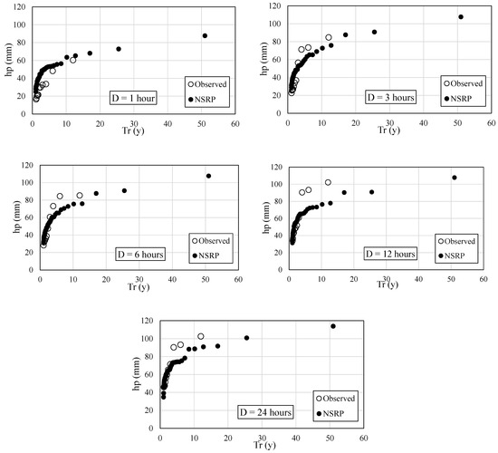
Figure 7.
Relationships, for different rainfall durations (D), among return periods (Tr) and cumulative values of annual maxima rainfall (hp).
Looking at Figure 7, the best performances of the model are obtained for D = 1, 3 and 6 h. Since a short duration (e.g., a few hours) rainfall is generally characterized by a high rainfall intensity, and since we are focusing here on soil erosion caused by extreme rainfall events, the obtained results seem to justify the use of the synthetic rainfall time series for R-factor calculation.
3.3. Comparison between Rainfall Erosivity Values Using Observed and Modelled Rainfall for the Station “Colli sul Velino”
Using the investigated 12 equations, a comparison between rainfall erosivity values obtained using synthetically generated and observed rainfall data has been conducted, in order to identify the most reliable equation to calculate rainfall erosivity in the study area.
Figure 8 shows, for all equations, the variability of R-factor for the Colli sul Velino rain gauge station. In the graph, average values of 12 simulated and observed data are shown, where the red line represents the average of 12 values obtained considering the synthetically generated rainfall data, while the black dashed line represents the average of 12 values obtained considering the observed data.
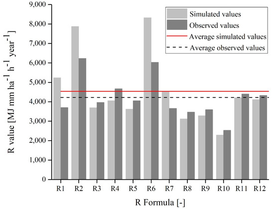
Figure 8.
Rainfall erosivity value obtained with the 12 investigated equations, respectively, with simulated and observed rainfall data set. The red line represents the average of 12 values obtained considering the synthetically generated rainfall data, while the black dashed line represents the average of 12 values obtained considering the observed data.
The dimensionless ratio between the rainfall erosivity value and its average value has been calculated for the simulated and observed rainfall data set. Through this dimensionless ratio, it was possible to establish, with the procedure described below, the degree of reliability of each equation.
The equation reliability degree can be high, medium or low. In particular, if the equation presents at least one of the following characteristics it will be assigned a low degree of reliability:
- Both values of columns 4 and 5 of Table 2 differ from the unitary value by +/−15%;
Table 2. Equation reliability degree based on rainfall erosivity values using simulated and observed rainfall for rain gauge station Colli sul Velino.
- Only one of the columns 4 and 5 of Table 2 differs from the unitary value by +/−15% and these values are opposite (for example one greater than the unitary value and the other smaller).
The degree of reliability is evaluated as "medium" if the following conditions are met:
- Only one of the columns 4 and 5 of Table 2 differs from the unitary value by +/−15%, but these values are both greater or smaller than the unitary value;
- Both the values of columns 4 and 5 of Table 2 differ from the unitary value by less than +/−15% and these values are opposite (for example one greater than the unit and the other smaller).
Finally, the degree of reliability is rated “high” if the following conditions are met:
- Both the values of columns 4 and 5 of Table 2 differ from the unitary value by less than +/−15%, but these values are both greater or smaller than the unitary value;
- Both the values of columns 4 and 5 of Table 2 differ from the unitary value by less than +/−10% and these values are opposite (for example one greater than the unit and the other smaller).
From the data reported in Table 2 we can conclude that:
- (i)
- the dimensionless ratio between rainfall erosivity values obtained using simulated rainfall and their average values only three times greater than 1 (equations no. 1-2-6), while the same ratio calculated with observed rainfall data is five times greater than 1 (equations no. 2-4-6-11-12). In general, in 8 times out of 12, the analysis on the observed rainfall data returns higher rainfall erosivity values; this aspect could be due to the larger sample data considered by modelled analysis.
- (ii)
- Equations no. 11 and 12 [41,42], both validated for Mediterranean zones, confirm a high reliability degree for the observed data set that, as said, is very small.
- (iii)
- Equation no. 7 [38] provides the better result for the synthetic data set. This demonstrates the adequacy of Yu and Rosewell’s equation for estimating the R-factor, one of the most used in international literature.
4. Conclusions
Intergovernmental Panel on Climate Change (IPCC) reports have shown higher precipitation projections, increasing the risk of soil loss by water runoff in the next century.
Therefore, evaluation of the rainfall erosivity is an important task, the determination of which affects the correct evaluation of soil erosion. In this paper, rainfall erosivity variability in the Rieti province of Central Italy has been investigated, analyzing 12 empirical formulas, suggested by literature, and using rainfall daily data observed from 2008 to 2018.
Starting from these premises, this work describes the efforts made to develop a methodology for rainfall erosivity evaluation in the case of ungauged or scarcely gauged areas. In fact, despite the fact that in the literature there are several equations to estimate rainfall erosivity, these two conditions represent a strong constrain to individuate the more reliable approach.
Results of numerical tests carried out for the Colli sul Velino rain gauge station were presented and discussed. In particular, the observed rainfall data were compared with numerical results obtained using a synthetic rainfall generator model developed by De Luca et al. [44,45,46,47,48]. Some peculiar features were observed.
The results reported in Figure 8 show consistent behavior across the three equations. In particular, it is interesting to note that equation no. 7 [38] represents one of the most used and one of oldest available in the literature. Particularly important are two other equations (no. 11 and 12) [41,42] that were developed for a Mediterranean habitat.
In our opinion, the use of a synthetic rainfall time series could help in solving the problem of hydrological data scarcity and consequently, guarantee major accuracy in estimating the R-factor for soil erosion evaluation.
Moreover, the availability of other rainfall data and the installation of new rain gauge stations in the Rieti province will make an upgrade of this work possible that could be seen as an interesting initial shift in the Lazio region’s soil loss management, which is still grounded in merely theoretical approaches.
Author Contributions
Conceptualization, A.P.; methodology, all authors; software, D.L.D.L.; writing—original draft preparation, A.P., D.L.D.L., C.A. and P.S.; writing—review and editing, all authors. All authors have read and agreed to the published version of the manuscript.
Funding
The Department for Regional Affairs and Autonomies (DARA), Presidency of the Council of Ministers, Rome (Italy), has co-financed this research. Number of Grant: DARA-DAFNE 40506.
Conflicts of Interest
The authors declare no conflict of interest.
References
- Beguería, S.; Serrano-Notivoli, R.; Tomas-Burguera, M. Computation of rainfall erosivity from daily precipitation amounts. Sci. Total Environ. 2018, 637–638, 359–373. [Google Scholar] [CrossRef] [PubMed]
- Xin, Z.; Yu, X.; Li, Q.; Lu, X.X. Spatiotemporal variation in rainfall erosivity on the Chinese Loess Plateau during the period 1956–2008. Reg. Environ. Chang. 2011, 11, 149–159. [Google Scholar] [CrossRef]
- Apollonio, C.; Petroselli, A.; Tauro, F.; Cecconi, M.; Biscarini, C.; Zarotti, C.; Grimaldi, S. Hillslope Erosion Mitigation: An Experimental Proof of a Nature-Based Solution. Sustainability 2021, 13, 6058. [Google Scholar] [CrossRef]
- Diodato, N.; Bellocchi, G. MedREM, a rainfall erosivity model for the Mediterranean region. J. Hydrol. 2010, 387, 119–127. [Google Scholar] [CrossRef]
- Wischmeier, W.H.; Smith, D.D. Predicting Rainfall-Erosion Losses from Cropland East of the Rocky Mountains. Guide for Selection of Practices for Soil and Water Conservation; Agriculture Handbook No. 282; US Department of Agriculture: Washington, DC, USA, 1965.
- Wischmeier, W.H.; Smith, D.D. Predicting rainfall-erosion losses: A Guide to Conservation Farming; Agricultural Handbook 537; US Department of Agriculture: Washington, DC, USA, 1978; pp. 1–151.
- Renard, K.G.; Foster, G.R.; Weesies, G.A.; McCool, D.K.; Yoder, D.C. Predicting soil erosion by water: A guide to conservation planning with the Revised Universal Soil Loss Equation (RUSLE); Agriculture Handbook No. 703; United States Department of Agriculture: Washington, DC, USA, 1997; p. 404.
- Foster, G.R. User’s Reference Guide. Revised Universal Soil Loss Equation Version 2 (RUSLE2); National Sedimentation Laboratory, USDA-Agricultural Research Service: Washington, DC, USA, 2004; p. 418.
- Lim, Y.S.; Kim, J.K.; Kim, J.W.; Park, B.I.; Kim, M.S. Analysis of the relationship between the kinetic energy and intensity of rainfall in Daejeon, Korea. Quat. Int. 2015, 384, 107–117. [Google Scholar] [CrossRef]
- Brown, L.C.; Foster, G.R. Storm erosivity using idealized intensity distribution. Trans. ASAE 1978, 30, 379–386. [Google Scholar] [CrossRef]
- Cecílio, R.A.; Moreira, M.C.; Pezzopane, J.E.M.; Pruski, F.F.; Fukunaga, D.C. Assessing rainfall erosivity indices through synthetic precipitation series and artificial neural networks. An. Acad. Bras. Ciências 2013, 85, 1523–1535. [Google Scholar] [CrossRef] [Green Version]
- Panagos, P.; Ballabio, C.; Borrelli, P.; Meusburger, K.; Klik, A.; Rousseva, S.; Tadić, M.P.; Michaelides, S.; Hrabalíková, M.; Olsen, P.; et al. Rainfall erosivity in Europe. Sci. Total Environ. 2015, 511, 801–814. [Google Scholar] [CrossRef] [Green Version]
- Isikwue, M.; Ocheme, J.; Aho, M. Evaluation of rainfall erosivity index for Abuja, Nigeria using Lombardi method. Niger. J. Technol. 2015, 34, 56. [Google Scholar] [CrossRef] [Green Version]
- Yu, B.; Hashim, G.M.; Eusof, Z. Estimating the R-factor with limited rainfall data: A case study from Peninsular Malaysia. J. Soil Water Conserv. 2001, 56, 101–105. [Google Scholar]
- Davison, P.; Hutchins, M.G.; Anthony, S.G.; Betson, M.; Johnson, C.; Lord, E.I. The relationship between potentially erosive storm energy and daily rainfall quantity in England and Wales. Sci. Total Environ. 2005, 344, 15–25. [Google Scholar] [CrossRef] [PubMed]
- Capolongo, D.; Diodato, N.; Mannaerts, C.M.; Piccarreta, M.; Strobl, R.O. Analyzing temporal changes in climate erosivity using a simplified rainfall erosivity model in Basilicata (southern Italy). J. Hydrol. 2008, 356, 119–130. [Google Scholar] [CrossRef]
- Gioia, A.; Lioi, B.; Totaro, V.; Molfetta, M.G.; Apollonio, C.; Bisantino, T.; Iacobellis, V. Estimation of Peak Discharges under Different Rainfall Depth–Duration–Frequency Formulations. Hydrology 2021, 8, 150. [Google Scholar] [CrossRef]
- Grimaldi, S.; Nardi, F.; Piscopia, R.; Petroselli, A.; Apollonio, C. Continuous hydrologic modelling for design simulation in small and ungauged basins: A step forward and some tests for its practical use. J. Hydrol. 2021, 595, 125664. [Google Scholar] [CrossRef]
- Ritschel, C.; Ulbrich, U.; Névir, P.; Rust, H.W. Precipitation extremes on multiple timescales—Bartlett–Lewis rectangular pulse model and intensity–duration–frequency curves. Hydrol. Earth Syst. Sci. 2017, 21, 6501–6517. [Google Scholar] [CrossRef] [Green Version]
- van Vliet, M.T.H.; Blenkinsop, S.; Burton, A.; Harpham, C.; Broers, H.P.; Fowler, H.J. A multi-model ensemble of downscaled spatial climate change scenarios for the Dommel catchment, Western Europe. Clim. Chang. 2012, 111, 249–277. [Google Scholar] [CrossRef] [Green Version]
- Blenkinsop, S.; Harpham, C.; Burton, A.; Goderniaux, P.; Brouyère, S.; Fowler, H.J. Downscaling transient climate change with a stochastic weather generator for the Geer catchment, Belgium. Clim. Res. 2013, 57, 95–109. [Google Scholar] [CrossRef] [Green Version]
- Forsythe, N.; Fowler, H.J.; Blenkinsop, S.; Burton, A.; Kilsby, C.G.; Archer, D.R.; Harpham, C.; Hashmi, M.Z. Application of a stochastic weather generator to assess climate change impacts in a semi-arid climate: The Upper Indus Basin. J. Hydrol. 2014, 517, 1019–1034. [Google Scholar] [CrossRef] [Green Version]
- Jones, P.D.; Harpham, C.; Burton, A.; Goodess, C.M. Downscaling regional climate model outputs for the Caribbean using a weather generator. Int. J. Climatol. 2016, 36, 4141–4163. [Google Scholar] [CrossRef] [Green Version]
- Yu, B. An assessment of uncalibrated CLIGEN in Australia. Agric. For. Meteorol. 2003, 119, 131–148. [Google Scholar] [CrossRef]
- Zhang, Y.-G.G.; Nearing, M.A.; Zhang, X.-C.C.; Xie, Y.; Wei, H. Projected rainfall erosivity changes under climate change from multimodel and multiscenario projections in Northeast China. J. Hydrol. 2010, 384, 97–106. [Google Scholar] [CrossRef]
- Blasi, C.; Capotorti, G.; Copiz, R.; Guida, D.; Mollo, B.; Smiraglia, D.; Zavattero, L. Classi-fication and mapping of the ecoregions of Italy. Plant Biosyst. 2014, 148, 1255–1345. [Google Scholar] [CrossRef]
- Bartolucci, F. Contributo alla conoscenza della flora dei monti carseolani (settore laziale): Monte Navegna (LAzio, Rieti). Inf. Bot. Ital. 2006, 38, 3–35. [Google Scholar]
- Anderlini, M.; De Santoli, L.; Fraticelli, F. Distributed Energy Generation: Case Study Of A Mountain School Campus In Italy. WIT Trans. Ecol. Environ. 2013, 73, 537–549. [Google Scholar]
- Porto, P. Exploring the effect of different time resolutions to calculate the rainfall erosivity factor R in Calabria, southern Italy. Hydrol. Process. 2016, 30, 1551–1562. [Google Scholar] [CrossRef]
- Mensing, S.A.; Schoolman, E.M.; Tunno, I.; Noble, P.J.; Sagnotti, L.; Florindo, F.; Piovesan, G. Historical ecology reveals landscape transformation coincident with cultural development in central Italy since the Roman Period. Sci. Rep. 2018, 8, 2138. [Google Scholar] [CrossRef] [Green Version]
- Wischmeier, W.H. A rainfall erosion index for a Universal Soil-Loss Equation. Soil Sci. Soc. Am. Proc. 1959, 23, 246–249. [Google Scholar] [CrossRef]
- Benavidez, R.; Jackson, B.; Maxwell, D.; Norton, K. A review of the (Revised) Universal Soil Loss Equation ((R)USLE): With a view to increasing its global applicability and improving soil loss estimates. Hydrol. Earth Syst. Sci. 2018, 22, 6059–6086. [Google Scholar] [CrossRef] [Green Version]
- Fournier, F.G.A. Climat et Erosion: La Relation Entre L’érosion du Sol par L’eau et les Précipitations Atmosphériques, 1st ed.; PUF: Paris, France, 1960. [Google Scholar]
- Arnoldus, H.M.J. An approximation of the rainfall factor in the Universal Soil Loss Equation. In Assessment of Erosion; John Wiley and Sons Ltd.: Hoboken, NJ, USA, 1980; pp. 127–132. [Google Scholar]
- Arnoldus, H.M.J. Methodology used to determine the maximum potential average annual soil loss due to sheet and rill erosion in Morocco. FAO Soils Bull. 1977, 34, 39–48. [Google Scholar]
- Lo, A.; El-Swaify, S.A.; Dangler, E.W.; Shinshiro, L. Effectiveness of EI30 as an erosivity index in Hawaii. Soil Conserv. Soc. Am. 1985. [Google Scholar]
- Renard, K.G.; Freimund, J.R. Using Monthly Precipitation Data to Estimate the R Factor in the Revised USLE. J. Hydrol. 1994, 157, 287–306. [Google Scholar] [CrossRef]
- Yu, B.; Rosewell, C.J. Technical notes: A robust estimator of the R-factor for the universal soil loss equation. Trans. ASAE 1996, 39, 559–561. [Google Scholar] [CrossRef]
- Ferrari, R.; Pasqui, M.; Bottai, L.; Esposito, S.; Di Giuseppe, E. Assessment of soil erosion estimate based on a high temporal resolution rainfall dataset. In Proceedings of the 7th European Conference on Applications of Meteorology (ECAM), Utrecht, Netherlands, 12–16 September 2005; pp. 12–16. [Google Scholar]
- Torri, D.; Borselli, L.; Guzzetti, F.; Calzolari, M.C.; Bazzoffi, P.; Ungaro, F.; Bartolini, D.; Salvador Sanchis, M.P. Italy. In Soil Erosion in Europe; Wiley: Chichester, UK, 2006; pp. 245–261. [Google Scholar]
- De Santos Loureiro, N.; De Azevedo Coutinho, M. A new procedure to estimate the RUSLE EI30 index, based on monthly rainfall data and applied to the Algarve region, Portugal. J. Hydrol. 2001, 250, 12–18. [Google Scholar] [CrossRef]
- Ferreira, V.; Panagopoulos, T. Seasonality of Soil Erosion Under Mediterranean Conditions at the Alqueva Dam Watershed. Environ. Manag. 2014, 54, 67–83. [Google Scholar] [CrossRef] [PubMed]
- Burton, A.; Fowler, H.J.; Blenkinsop, S.; Kilsby, C.G. Downscaling transient climate change using a Neyman-Scott rectangular pulses stochastic rainfall model. J. Hydrol. 2010, 381, 18–32. [Google Scholar] [CrossRef]
- De Luca, D.L.; Galasso, L. Calibration of NSRP Models from Extreme Value Distributions. Hydrology 2019, 6, 89. [Google Scholar] [CrossRef] [Green Version]
- De Luca, D.L.; Petroselli, A.; Galasso, L. Modelling Climate Changes with Stationary Models: Is It Possible or Is It a Paradox? In Numerical Computations: Theory and Algorithms. NUMTA 2019; Lecture Notes in Computer Science (Including Subseries Lecture Notes in Artificial Intelligence and Lecture Notes in Bioinformatics); Springer: Cham, Switzerland, 2020; Volume 11974, pp. 84–96. [Google Scholar]
- De Luca, D.L.; Petroselli, A.; Galasso, L. A transient Stochastic Rainfall Generator for climate changes analysis at hydrological scales in Central Italy. Atmosphere 2020, 11, 1292. [Google Scholar] [CrossRef]
- De Luca, D.L.; Petroselli, A. STORAGE (STOchastic RAinfall GEnerator): A user-friendly software for generating long and high-resolution rainfall time series. Hydrology 2021, 8, 76. [Google Scholar] [CrossRef]
- Recanatesi, F.; Petroselli, A.; Ripa, M.N.; Leone, A. Assessment of stormwater runoff management practices and BMPs under soil sealing: A study case in a peri-urban watershed of the metropolitan area of Rome (Italy). J. Environ. Manag. 2017, 201, 6–18. [Google Scholar] [CrossRef] [PubMed]
Publisher’s Note: MDPI stays neutral with regard to jurisdictional claims in published maps and institutional affiliations. |
© 2021 by the authors. Licensee MDPI, Basel, Switzerland. This article is an open access article distributed under the terms and conditions of the Creative Commons Attribution (CC BY) license (https://creativecommons.org/licenses/by/4.0/).