Article

Implications of a Priori Parameters on Calibration in Conditions of Varying Terrain Characteristics: Case Study of the SAC-SMA Model in Eastern United States

1
Department of Fisheries and Oceans, 343 Université Ave, Moncton, NB E1C 5K4, Canada
2
Forest Sciences Centre 2030, University of British Columbia, 2424 Main Mall, Vancouver, BC V6T 1Z4, Canada
3
Coweeta Hydrologic Lab, Center for Forest Watershed Research, Southern Research Station, USDA Forest Service, 3160 Coweeta Lab Road, Otto, NC 28734, USA
*
Author to whom correspondence should be addressed.
Hydrology 2021, 8(2), 78; https://doi.org/10.3390/hydrology8020078
Submission received: 17 March 2021 / Revised: 29 April 2021 / Accepted: 1 May 2021 / Published: 11 May 2021

Abstract

:
This study seeks to advance the knowledge about the effect of a priori parameters on calibration using the Sacramento Soil Moisture accounting Model (SAC-SMA). We investigated the catchment characteristics where calibration is most affected by the limitations in the a priori parameters and we studied the effect on the modeled processes. The a priori parameters of SAC-SMA model parameters were determined from soil-derived physical expressions that make use of the soil’s physical properties. The study employed 63 catchments from the eastern United States (US). The model calibration employed the Shuffle-Complex algorithm (SCE-UA) and used the a priori parameters as default allowing for ±35% as a range of deviation. The model efficiency after calibration was sensitive to the catchment landscape properties, particularly the soil texture and topography. The highest efficiency was obtained in conditions of well-drained soils and flat topography where the saturation excess overland flow is predominant. Most of the catchments with smaller efficiency had poorly drained soils where mountainous and forested catchments of predominant subsurface stormflow had the lowest efficiency. The current regional study shows that improvements of SAC-SMA a priori parameters are crucial to foster their operational use for calibration and prediction at ungauged catchments.

1. Introduction

There has always been a need to understand the hydrological behavior of catchments at the regional scale because it drives the decisions of water resource planners and managers [1]. The regional evaluation of runoff processes and streamflow pattern provides some degree of predictability of the catchments’ behavior [2,3]. Streamflow analysis at a regional scale entails the use of hydrological modeling. The uncertainty due to model calibration and parameter estimation is among the challenges of hydrological modeling [4,5,6,7,8].
The technique of a priori parameter estimation was designed to facilitate the model parameterization and calibration [9]. The a priori parameters derive values directly from spatiotemporal data. The technique recourses to establishing “physical” or “conceptual” correlations between measured watershed characteristics (e.g., geology, topography, soils, and land cover, etc.) and the parameters to represent the hydrological processes of the model [10].
The a priori parameters can be used to minimize the number of parameters to calibrate, to estimate parameters when calibration is not possible (ungauged catchments conditions), and to guide the model calibration in accordance with a parameter range [11]. While the estimate of a priori parameters is far from being perfect, it has been receiving increased attention from hydrologists and water resources managers e.g., [9,12,13,14,15].
Though a priori parameters’ estimation was initiated decades ago, it remains available only for few hydrological models, e.g., [9,16]. The authors of [17] developed empirical equations to correlate the VIC-2LLSM parameters to basin features. In [12], the authors correlated the parameters of the Simple Water Balance (SWB) model to catchments’ features in the southeast of the United States (US). The authors of [18] related 16 parameters of the conceptual Tank model to land use and soil types using multiple linear regressions. The regressions had limited success. First, because the correlation between the catchment characteristics (e.g., the soil hydraulic properties and the soil depth) and the model parameters is indirect. Second, the calibrated parameters that were used to develop the regressions induced uncertainty in the relationships, e.g., [11,19].
The authors in [9] employed geographically based information (topography, soil data, land use/land cover data, etc.) to estimate spatially varied parameters of the GXM model (spatially distributed Grid-Xinanjiang model).
In physically-based distributed models, the a priori parameters are often directly measured. This strategy implies a lack of accuracy in situations of major inconsistencies between the sampling spatial resolution and the size of the grid used to conduct the model calibration [20,21]. It has always been questioned whether there is consistency between what we can measure/observe in terms of parameters and whether this responds to the model complexity [22]. Some parameters in models are difficult to measure. The lack of consistency between what can be measured and what the model requires should not urge us to opt for less complex models [23]. The Sacramento Soil Moisture Accounting Model (SAC-SMA) is among the few lumped models that have soil-derived a priori parameters. These parameters are the outcome of analytical and empirical equations [23]. The lumped SAC-SMA model is well suited to conduct regional studies because (i) lumped models are parsimonious [24], (ii) the a priori expressions of SAC-SMA parameters employ a physically realistic technique that is applicable worldwide [6,23], and (iii) the spatially-explicit soil data are widely available at resolutions appropriate for regional assessments.
One area worth investigating is the implications of a priori parameters on SAC-SMA predictions and calibration. There will be a great gain of knowledge if a regional framework is adopted as the analysis will benefit from the variability in hydrological and physiographic characteristics of the catchments. The a priori parameters are derived from a globally applicable approach. Therefore, the wider community will also gain insights into the design of a priori parameters and the aspects leading to model deficiency.
Within the framework of the Model Parameter Experiment (MOPEX), the SAC-SMA a priori parameters have been estimated in several catchments across the continental United States [25]. All a priori parameters are soil derived and used the State Soil Geographic Database (STATSGO) map to estimate θwlt (the water content at wilting point), θs (the water content at saturation), θfld (the water content at field capacity), and Ks (the hydraulic conductivity at saturation) [12,23]. In the eastern United States and using a small number of catchments from the mid-latitudes, [23] found that flow simulation from a priori parameters led to similar model efficiencies as the calibrated parameters. The use of a priori parameters in calibration helps to retain physical consistency and reduce equifinality [13,23]. The study by [26] obtained non-satisfactory predictions using a few geographically distant MOPEX catchments in the US. The uncertainty in values of a priori parameters used to calibrate the model would have been transferred to the calibrated parameters. The limited number of catchments used in [23,26] are not sufficient to make a statement about the use of a priori parameters in SAC-SMA calibration.
The SAC-SMA model efficiency might be closely dependent on catchments’ physiography given that a priori parameters—used to conduct the calibration—are based on the hydraulic properties of the soil. Whether the calibration based on a priori parameters captures the effect of the changing terrain characteristics on the hydrological response is unknown. There is a need to identify the catchment conditions leading to low (high) efficiency after SAC-SMA calibration.
Therefore, the objectives of the current study are:
(i) to reveal the effect of variation in terrain characteristics on SAC-SMA predictions, using a priori parameters and calibrated parameters (ii) to understand the effect of SAC-SMA a priori parameters on the modeled processes in conditions of varying physiography. The study also explores and discusses the opportunities to improve the SAC-SMA predictions after a priori parameters-based calibration.
This investigation remains a case study of the SAC-SMA model. Hence, it does not intend to generalize the outcomes to all models for which a priori parameters had been designed. Nonetheless, the study provides insights on how to better conceive and set a priori parameters in order to improve hydrological modeling and storm flow forecasting. Being a regional study, this investigation advances our understanding about the effect of catchment characteristics on models’ performance. In addition, it underlines the aspects to be cautious of when using the a priori parameters in hydrological modeling.

2. Database and Study Area Characteristics

The MOPEX database contains historical hydrometeorological data and land surface characteristics for many hydrological basins in the US and in other countries [6]. MOPEX research has been driven by a series of international workshops that brought together interested hydrologists and modelers to exchange knowledge and experience in developing and applying model parameter estimation techniques. With its focus on parameter estimation, MOPEX plays a major role in the context of international initiatives, such as Prediction in Ungauged Basins (PUB) [27]. Our regional study used 63 MOPEX catchments in the eastern United States where the mean annual precipitation (MAP) varies between 702 mm and 2072 mm (Table 1). The catchments range in size from 67 km2 to 8052 km2 (Table 1) (20% of the catchments have sizes above 4000 km2).
Daily time series of streamflow, areal averaged precipitation, and potential evapotranspiration (PET) for all study catchments were provided by the MOPEX project [9]. The database is freely available and was retrieved from the following website: https://hydrology.nws.noaa.gov/pub/gcip/mopex/US_Data/Us_438_Daily/ (accessed on 10 May 2021). In MOPEX, the data available are precipitation, potential evapotranspiration, flow, maximum air temperature, and minimum air temperature. The time step for the MOPEX data is daily. There is a readme.txt file that provides a detailed description of the data available. The list of the stations from this study can be found in the supplementary excel file. The excel sheet name is “Study Stations”.
The precipitation was determined by means of weighted averaging using rain gages’ measurements and PRISM data [14]. The PET was estimated on the basis of the NOAA Evaporation Atlas. The NOAA Atlas maps were derived by analysis of evaporation pan data [14]. The perennial snow cover was absent for most catchments [28]. The mean monthly depths of precipitation across the study catchments were comparable and had limited fluctuations throughout the seasons [28]. However, the storm characteristics, in particular, the storm intensity, had systematic seasonal variations [29]. The catchments within the study area were mostly forested and were minimally impacted by human influences [28].
In the study region, the Appalachian Mountains created a contrast in the topography. The catchments with low relief were primarily located on the east coast and in the State of Georgia, while the interior catchments had higher relief. The maximum elevation across the region was 2029 m.a.s.l. (meters above sea level) (Figure 1). The variation in soil texture across the study catchments affects the soil hydrologic characteristics [30]. Figure 1 shows the spatial change in the main hydrologic groups: HGB (soil with medium infiltration rate) and HGC (soil with slow infiltration rate). There is a gradual decrease in HGB soils from south to north. In mid-latitudes, the soil is a combination of HGB and HGC, while in the northeast it is predominantly the HGC group. The soil group HGA (soil with high infiltration rate) is also present in eastern United States primarily in the state of West Virginia.

3. Materials and Methods

Given the regional aspect of the study, the criterion of homogeneity in the hydrologic response was considered through the use of homogeneous regions in eastern US [31]. The idea behind working in homogeneous regions was to allow for model efficiency comparison between the regions and within the same region. The criteria of homogeneity facilitated the study of a priori parameter effect on model performance and on calibration. The analysis used the regionalization of [32]. Within each region, each MOPEX catchment had a set of a priori parameters that was used to make a first prediction. This first prediction used the same record length as that used to conduct the model calibration (1948–1963). This prediction was denoted as the APRIORI phase (step 1 in Figure 2). The model was then calibrated using the SCE-UA algorithm (record length 1948–1963). The a priori parameters were the starting values to conduct the calibration (step 2 in Figure 2). This phase was denoted as CAL and generated a set of calibrated parameters (step 3 in Figure 2). CAL and APRIORI both used the same record length for consistency. Each catchment of the same region had a set of a priori parameters and a set of calibrated parameters. The model efficiency was measured in each region using the a priori and calibrated parameters applied on the same MOPEX data during the calibration period (1948–1963) and the validation period (1964–2000) (please check Section 3.2.2 for more about calibration, validation, and model efficiency metrics) (step 4 in Figure 2).
The value of each parameter varied among catchments of the same region. The variability of each a priori parameter among catchments of the same region was quantified. After calibration, the variability of the same parameter was also quantified. The level of variability of the model parameters was compared between the APRIORI and CAL phases (step 5 in Figure 2). If the variability of one specific parameter from APRIORI to CAL increased in one region, then the calibration better mimicked the variability of that parameter value among the catchments of the same region. The parameter was then considered among the parameters most influential on the prediction. The criteria of increased variability was previously used in [23,26]. The physical meaning of each parameter having an increase in variability from APRIORI to CAL tells about the hydrological processes mostly driving the runoff prediction. If the parameter variability is stable between APRIORI to CAL, then the calibrated parameters barely changed from the a priori values after calibration.
The topographic index (TI) distribution at the catchment scale in eastern United States, analyzed in [33], was used to determine the dominant runoff generation mechanisms in each catchment for this study. The dominant runoff generation mechanisms, the prediction efficiency, the parameters’ physical meaning and nuances in their variability between APRIORI and CAL allowed the exploration of the a priori parameters’ performance and their implication on SAC-SMA calibration (step 6 in Figure 2).

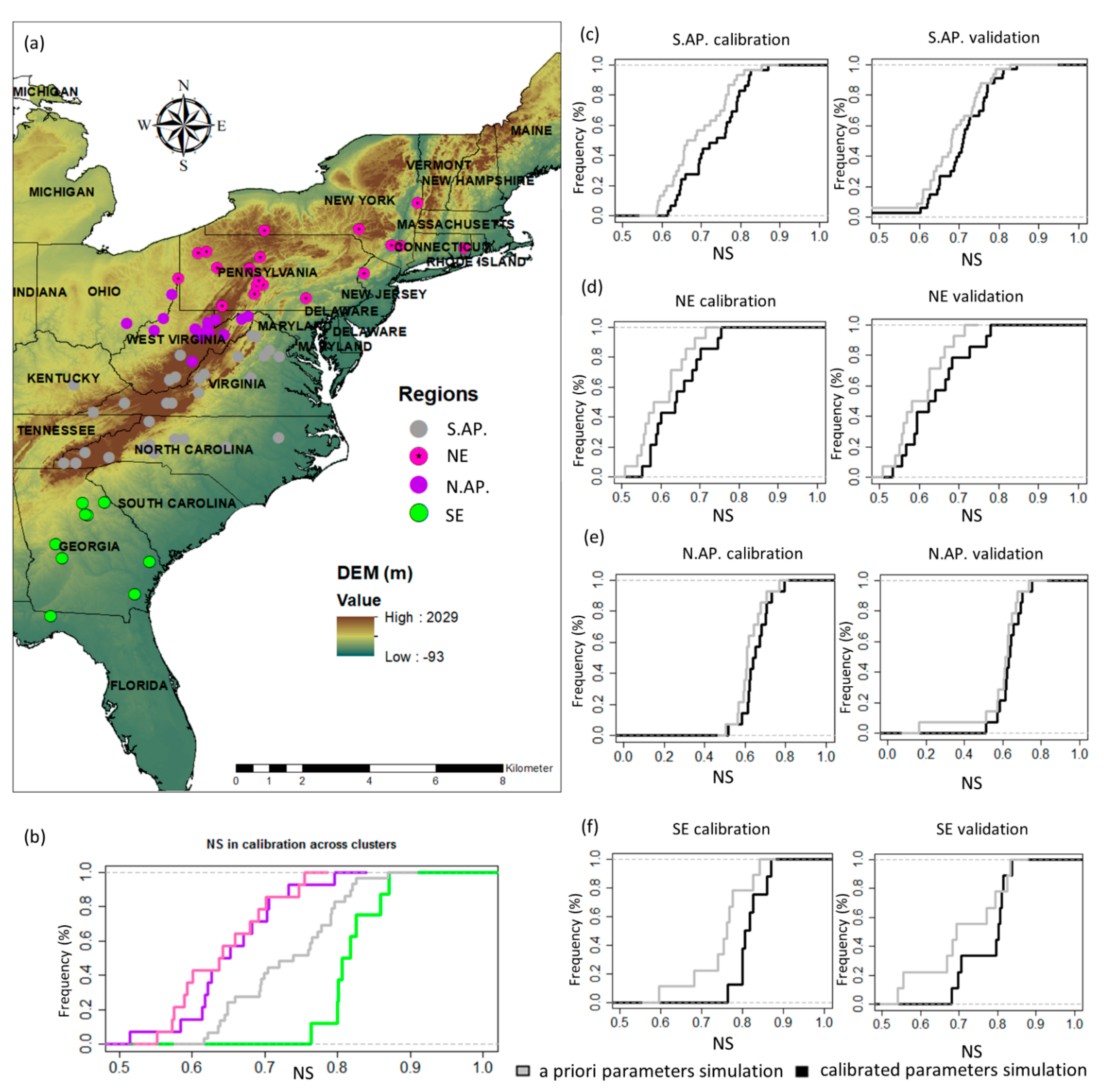
3.1. Catchment Classification

According to [30], a classification should be physically meaningful and provide a means to assess the dominant controls on the streamflow patterns [34]. Ideally, it reveals some understanding of the catchment’s hydrologic partition function (interception, infiltration, and percolation) and the storage function (vegetation, depression, retention, groundwater, and snowpack) [30]. In this paper, we used the catchment classification of [31], which subdivides the study region into four regions with similar hydrologic responses. This classification disclosed the dominant runoff processes in each region using six hydrologic signatures: the baseflow index, runoff ratio, slope of FDC (Flow Duration Curve), streamflow elasticity to precipitation, hydrograph rising limb, and snow day ratio. The novelty of the classification in [31] is not in the signatures themselves but in their combination to quantify the hydrologic function and, therefore, the hydrologic similarity between the catchments. For the purposes of this study, we refer to Southern Appalachian as S.AP., Northeast as NE, Northern Appalachian as N.AP., and Southeast as SE.

3.2. SAC-SMA Model Structure and Calibration

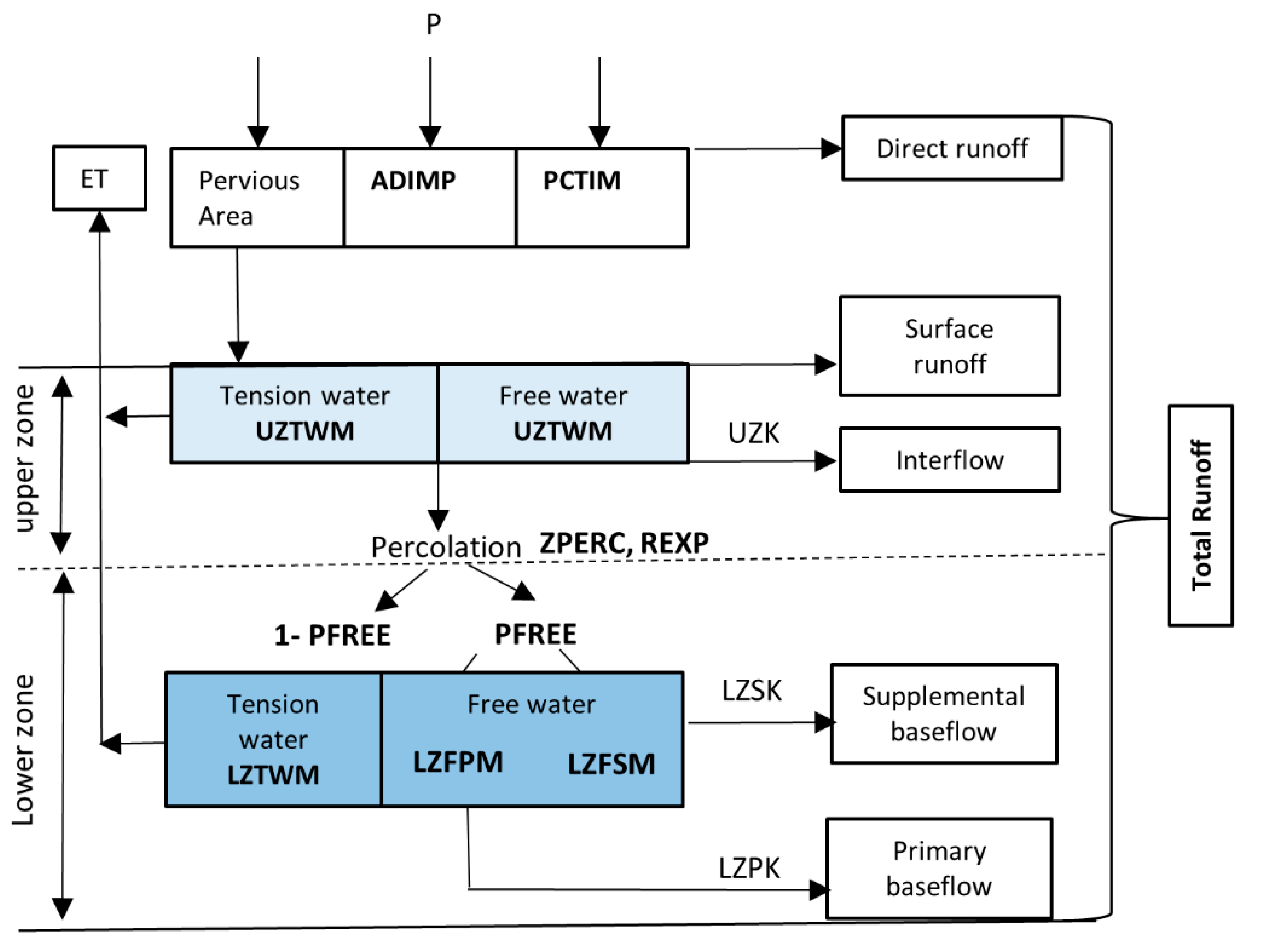
3.2.1. Model Parameters and Physical Meaning

The SAC-SMA model has been applied worldwide, particularly in the different hydroclimate regimes of the United States [23].
The SAC-SMA conceptual model allows for detailed flow simulations dealing with runoff components, i.e., the direct runoff, surface runoff, interflow, and baseflow [35]. The model has a two-soil-layer structure (Figure 3). Each layer is made of tension and free water storages that interact to simulate soil moisture and five runoff components [23,26]. The tension water storages simulate the evapotranspiration (ET). The daily average PET from MOPEX data is one of the inputs necessary for ET simulations. The free water storage of the lower layer has two sub-storages that simulate supplemental (fast) and primary (slow) groundwater flows (Figure 3).
The storage in the tension and free water of the upper zone partitions the rainfall into surface runoff and infiltration into the lower zone storage. The model had 13 parameters in total that are explicitly described in Table 2.
The excess from the tension water capacity of the upper zone (UZTWM) becomes the excess rainfall, and the excess from above the free water capacity (UZFWM) generates the surface runoff. At saturation of the upper zone storages, the runoff rate is influenced by deficiencies in the lower zone reservoirs, the tension water, LZTWM, and the free water, LZFSM and LZFPM, capacities. The runoff is generated at each free water reservoir depending on the depletion coefficients, namely, the UZK coefficient in the upper zone and LZSK and LZPK in the lower zone (see Figure 3). The percolation rate into the lower zone is a nonlinear function of the deficiencies of the lower and upper reservoirs and includes two parameters: the maximum rate of percolation, ZPERC, and an exponent value, REXP [24]. The water from the deep percolation divides into three storages. The PFREE parameter determines the fractional split between the tension and free water storages. The parameters not estimated by the a priori expressions are ADIMP and PCTIM because they are not soil-derived [24].

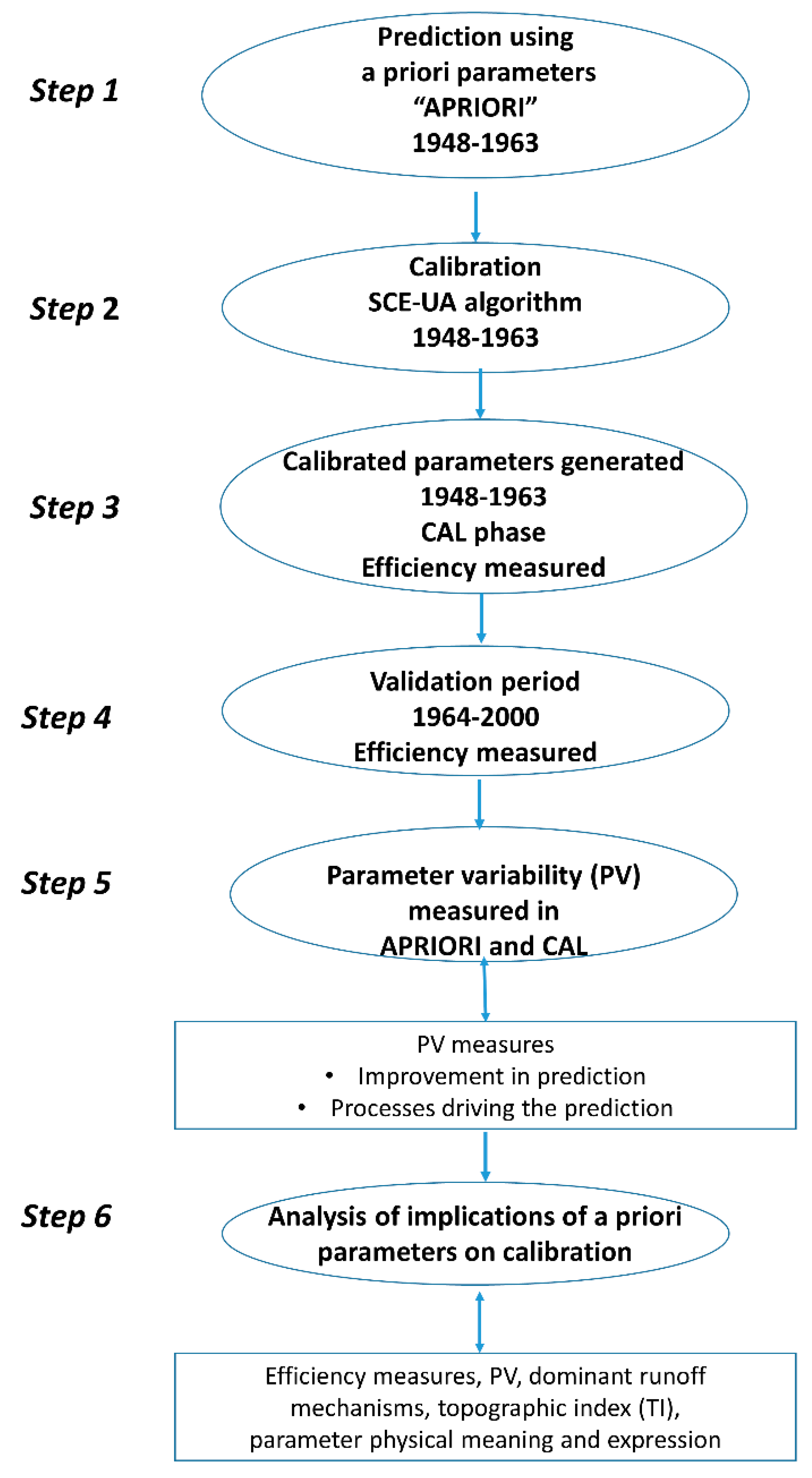
3.2.2. SAC-SMA Calibration and Validation

SAC-SMA Calibration

We calibrated the thirteen SAC-SMA model parameters using the Shuffle Complex algorithm (SCE-UA) with 10,000 iterations [36]. The calibration period used flow data and precipitation from 1948–1963. The SCE-UAE algorithm is extensively used as an optimization approach that identifies global optimums. The SCE-UA algorithm helped achieve different research goals, such as studying model parameter transferability (e.g., [26,32]) and building a large database for the continental United States (e.g., [37]).
Calibration within the Bayesian framework through the Monte Carlo (MCMC) approach is also popular in hydrological modeling. It provides a probabilistic framework that addresses model and parameter uncertainties [38]. However, convergence of the method may be problematic in the case of inappropriate selection of the posterior distribution to quantify the parameters. The calibration may be trapped in local posterior modes [39]. There are efforts to solve—to some extent—the issues of “global” and “local” posterior modes within the Bayesian framework [40]. For the current study, we did not use the Bayesian framework but rather we opted for an optimization approach that is well suited for the SAC-SMA model, as shown recently in [37]. In SCE-UA, the search space for the parameters set is made of complexes. The criteria of dependence between the parameters of the same set is implicit in the search [41]. The population of points are spread over complexes where each evolve independently into an improvement direction. Shuffles are repeatedly performed and the points are reassigned to complexes. As the search progresses, there is convergence toward the global optimum [42].
Similar to [23,26], we used a constrained range of parameters centered on the a priori estimates to maintain physical consistency and to reduce equifinality after calibration. So, the starting value to conduct the calibration was the a priori value of each parameter. We set ±35% as the range of deviations allowed from the default parameters (a priori parameters). This range was larger than the range used in [23] (i.e., ±25%). We set this range in order to allow for more parameters’ variability—around the a priori values—that is used by the SCE-UA algorithm to find the global optimum. The model was calibrated for the period 1948–1963. The objective function minimized RMSE (Root Mean Square Error) between daily observed and simulated discharges.
RMSE = i = 1 n   P i O i 2 n
i: Variable i, I = 1, ..., n;
P: Predicted value of the discharge;
O: Observed value of the discharge;
n: The total number of observations during the simulation period.
There are growing concerns regarding the suitability of performance metrics to meet particular goals in rainfall–runoff modeling and their ability to describe the overall model performance (e.g., [43,44,45]). The RMSE (absolute differences between observed and modeled values in their original unit) is regarded as one of the metrics that well describes the performance of rainfall–runoff modeling ([45,46]). The lower the RMSE the better is the fit. For further evaluation and performance illustration, we used the Nash–Sutcliffe coefficient (NS) [46] and the percentage bias (PBIAS) in mean flow [47]. A better fit is associated with a lower PBIAS and a larger NS. In order to allow for comparison, we used the same metrics to evaluate the efficiency during the calibration phase using the a priori parameters.

SAC-SMA Validation

Once the model calibration was accomplished and the values of calibrated parameters were obtained, the model predictions were further tested during the validation period. The major concern about validation is the approach used by the modeler to conduct this test of the model efficiency. Usually, in hydrological modeling we use either the cross validation method or the split sample method [48]. In the former approach (cross validation), the model validation is alternated with the calibration via a machine learning tool (i.e., MCMC approach). In the split sample approach, the total length of the flow data are split into two periods; (i) the calibration period, which is a period of the flow record that is used to run the calibration algorithm in order to determine the model parameters that lead to a best fit (lower RMSE, lower PBIAS, and larger NS), (ii) the validation period employs the rest of the flow data to test the model prediction using the same metrics (RMSE, PBIAS, NS) for consistency. Usually, the flow record employed in the validation phase is longer. In this study, the validation period spanned over 1964–2000.The efficiency from the prediction using a priori parameters was also quantified during the validation period. The efficiency metrics helped to compare between the predictions using the a priori and calibrated parameters. The validation phase allowed testing the efficiency of the calibrated and a priori parameters during a different period of the flow record. The split sample approach is intensively used in hydrological modeling and is called [48].

4. Results

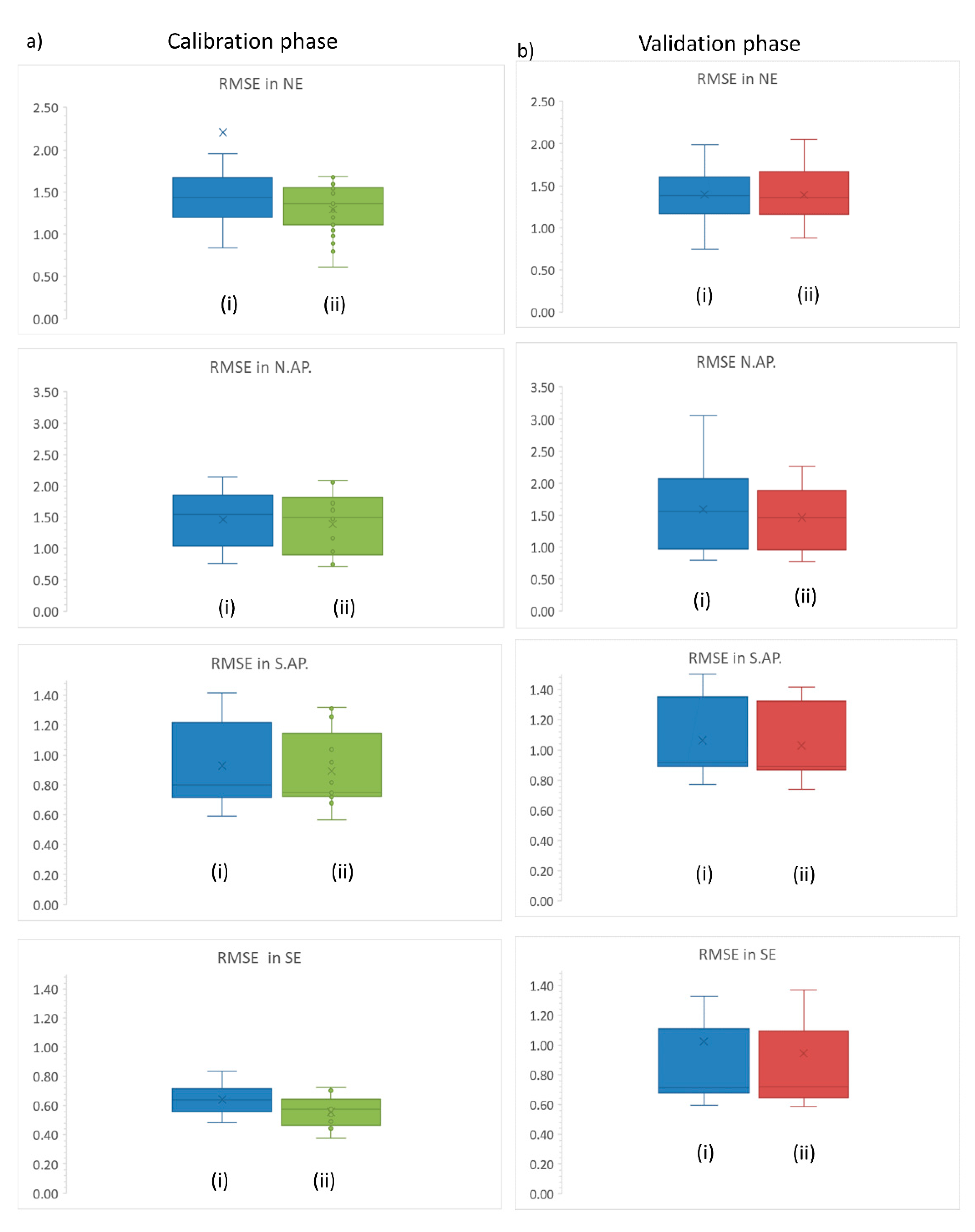
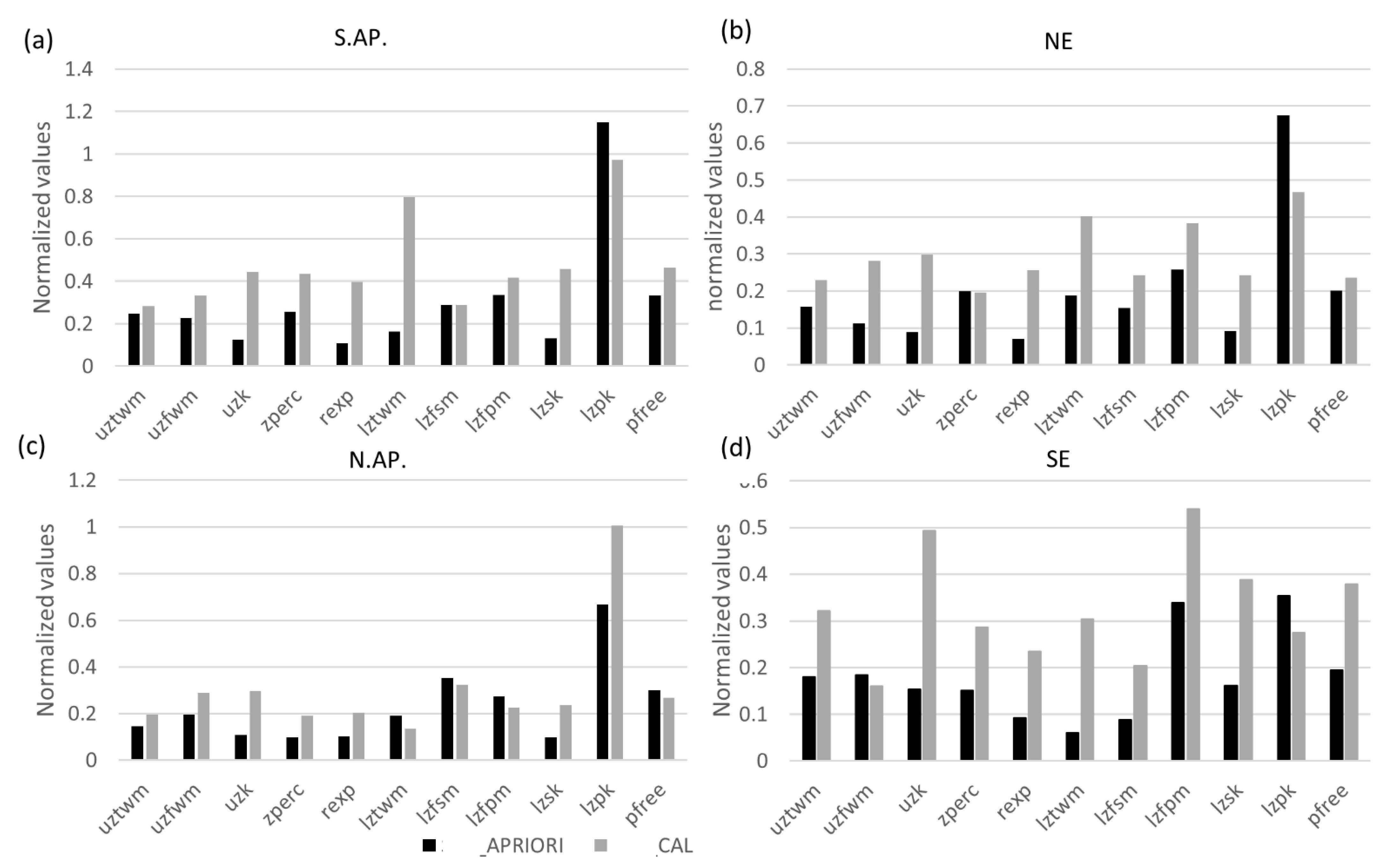
4.1. Model Performance Using A Priori and Calibrated Parameters

The study regions are presented in Figure 4a, and the results of model calibration are summarized in Figure 4 and Figure 5. The cumulative distribution function (CDF) of the NS coefficients showed that the best performance at calibration was in SE and S.AP. The catchments with the poorest performance were in N.AP. and NE (Figure 4b). According to Figure 4, the major improvements from APRIORI to CAL simulations were observed in S.AP., NE, and SE Figure 4c,d,f, respectively). The same pattern of improvement was observed in the validation phase as well.
The RMSE as specified in Equation (1) measures the errors in simulations using observed and predicted discharges at each study station. In Figure 5, we present the results of RMSE per region and per simulation period; panel (a) provides results for the calibration period (1948–1963). Panel (b) presents results for the validation period (1964–2000). In each simulation period the efficiency was evaluated using the a priori parameters (boxplots (i)) and the calibrated parameters (boxplots (ii)). The criteria of a better fit entails that the lower the RMSE, the higher is the model performance. The RMSE decreased the most during calibration period for S.AP., NE, and SE (Figure 5a). For the validation period, the RMSE in these regions remained lower than the values obtained using the a priori parameters during the same test period (Figure 5b). It is worth noting that in NE, at validation, the RMSE did not differ much between the a priori and calibrated parameters (Figure 5b). The NS of the calibration and validation periods in N.AP. barely improved compared with the a priori parameters (Figure 4e). The RMSE did not remarkably decrease between the a priori and calibrated parameters (Figure 5 for N.AP. region). Nonetheless, the calibration assured the maintenance of the model efficiency higher than 0.5 after the validation though the simulations using a priori parameters dropped to 0.2 in one study catchment (see Figure 4e).

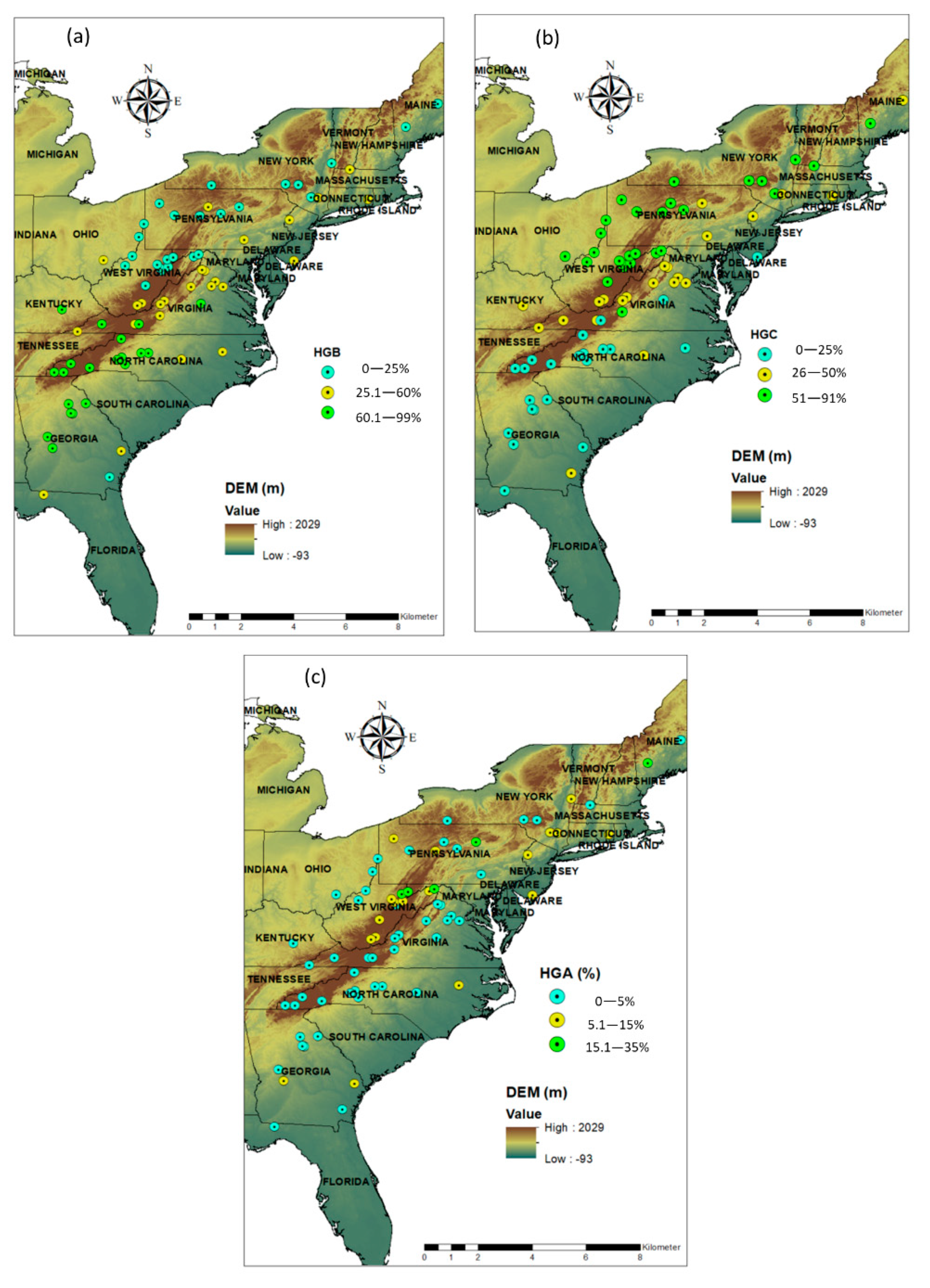
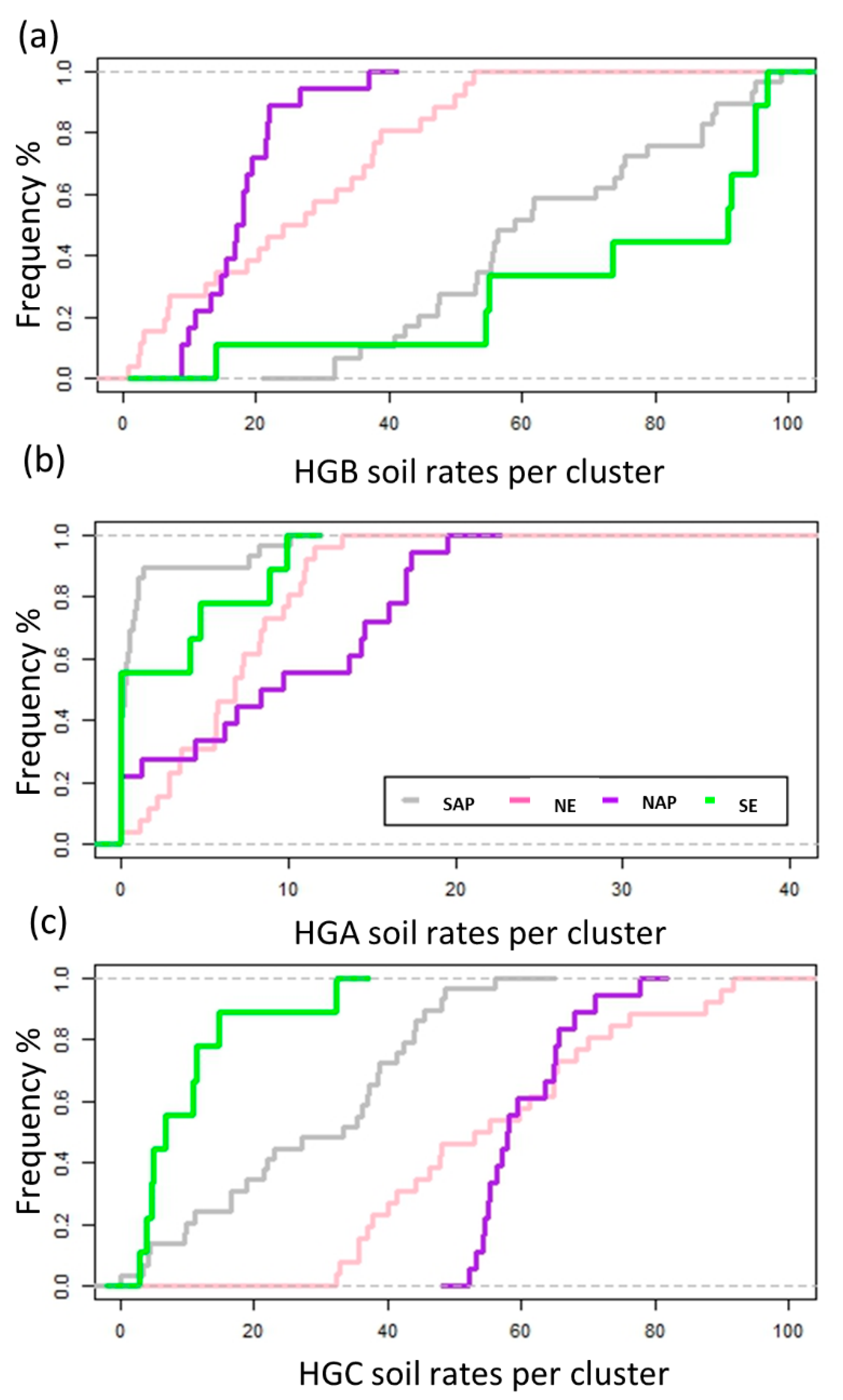
4.2. Analysis of Predictions from A Priori Parameters and Calibration: The Catchment Land Scape Properties and Runoff Processes

In NE and N.AP., the soils are poorly drained and have a steep topography, whereas, in SE, the catchments have well-drained soils and are located at lower elevations (Figure 4a). In Figure 6, large differences were observed in the spatial patterns of the soil hydrologic groups. The CDFs of HGB showed that it was predominant in SE and S.AP. (Figure 6a). The proportion of HGA soils was small across regions (soils with high infiltration, Wood et al. 1984 [30]), except in N.AP. (Figure 6b). Meanwhile, HGC soils (slow infiltration rate) were prominent in N.AP. and NE (Figure 6c).
The CDFs of HGB showed that it was predominant in SE and S.AP. (Figure 6a). The proportion of HGA soils was small across regions (soils with high infiltration, Wood et al., 1984), except for N.AP. (Figure 6b). Meanwhile, HGC soils (slow infiltration rate) were large in proportions in N.AP. and NE (Figure 6c).
According to Table 3, in S.AP. as the percent of the HGB soils rose, the model efficiency in each catchment improved for APRIORI and CAL simulations. The increase in fine soil textures proportions (HGC and HGBD (slow infiltration rate according to Wood et al., 1984)) affected the model efficiency in APRIORI and CAL. The correlations of the NS coefficient with the different soil hydrologic groups were statistically significant (p-value < 0.05).
At calibration, in S.AP., the main improvements were associated with an increase in variability of deep percolation parameters (ZPERC, REXP in Figure 7a) and depletion from free water storage in the upper layer (UZK, Figure 7a), which implied additional water leakages from the interflow and improved infiltration toward the lower layers were achieved after calibration. The increase in LZTWM variability (see Section 3.2.1 for physical meaning) suggested that the deep percolation permitted for additional evapotranspiration from the lower layer.
In NE region and according to Table 3, the increase in the HGA and HGB soil proportions increased the model efficiency. This effect was not statistically significant (p-value > 0.05). However, the increase in the HGC soils decreased the NS coefficients in APRIORI and CAL (p-value < 0.05). After calibration, the effect of the fine soil texture on the model performance was adjusted by increasing the variability of the deep percolation parameters (UZK and REXP in Figure 6b). Therefore, additional water was needed to move downwards to increase the evapotranspiration from the deep soils (more variable LZTWM after calibration in Figure 7b).
As for N.AP., the results of the correlations in Table 3 indicated that the model performance improved in APRIORI and CAL as the amount of HGA soils decreased (p-value < 0.05). The effect of HGC and HGB soils was not statistically significant (p-value > 0.05). In Figure 6c, the depletion coefficient from the lower layer (LZPK) was the most variable parameter in both simulations. The variability of the drainage parameter from the upper layer and its depletion coefficient (UZFWM and UZK, respectively) slightly increased after calibration.
In SE (located in the State of Georgia), APRIORI was affected by HGA soils but more significantly by HGB and HGC soils (p-value < 0.05 in Table 3). The model efficiency improved as the HGB soils increased (p-value < 0.05). After calibration, the parameters responsible for the subsurface processes increased in variability, e.g., UZK, ZPERC, and REXP (Figure 7d). In addition, the baseflow contribution was enhanced due to an increase in the LZFPM and LZSK variability (the lower layer depletion coefficients in Figure 7d).
In S.AP., SE and in most catchments from NE, the saturation excess is predominant, according to Chouaib et al. (2018) (see Figure 6 in this manuscript). This was where the parameters simulating the model processes of deep percolation had the highest variability (particularly in S.AP. and NE) and those responsible of baseflow, particularly in SE, increased in variability after calibration. In N.AP., all the catchments are at high altitudes in the Appalachians (Figure 7). In N.AP. the catchments were dominated by the subsurface stormflow. In these catchments, the parameters responsible for interflow had the highest variability after calibration.

5. Discussion

This regional study evaluated the use of a priori parameters to facilitate the SAC-SMA model calibration and predictions. It also examined the effect of a priori parameters—when used either for prediction or calibration—on the modeled processes. The analysis revealed the catchment characteristics for which the predictions were less efficient.
The results demonstrated that CAL efficiency was low in catchments with poorly drained soils. The highest efficiency using a priori parameters without calibration was in SE (in Georgia). After calibration (CAL), the efficiency from catchments in S.AP. and NE was less important than in SE (Figure 4c,d,f, respectively). The poorest efficiency after calibration was found in NE and N.AP. NE and N.AP. are regions with slow infiltration rates (large proportions of HGC soils, Figure 1). The differences in efficiency across the regions suggested that in catchments with finer soil texture, the flow simulation is challenging. The a priori parameters of SAC-SMA guided the calibration. Therefore, some of the uncertainty in the a priori parameters may have been transferred to the calibrated parameters. Lower efficiency of APRIORI and CAL phases found in S.AP., NE, and N.AP entails that the uncertainty of a priori parameter was pronounced in poorly drained soils of the eastern US.
The physiographic characteristics of catchments in SE, primarily low relief and well-drained soils were an indication of large water infiltration. In SE (Georgia), the increase in the variability of all parameters after calibration (Figure 7d) pointed to improved representation of the differences in soil properties among the catchments of the same region compared to a priori parameters results (see the average NS coefficients in SE for APRIORI and CAL). Remarkably, the groundwater processes were prevalent in SE due to relatively large variability in LZFPM (a parameter responsible for drainage from the lower layer to baseflow). The prevalent groundwater processes agreed with results from [32] with regard to topographic index (TI) in SE; the saturation excess overland flow was predominant in this region (see Figure 11 in [32]). In SE, the increase in LZFPM variability after calibration referred to a better representation of the differences in groundwater effect between the catchments. The lower layer a priori parameters did not have the same level of variability, which hints at an increased uncertainty. This is of particular interest to catchments with deep groundwater, such as those of SE. The soil information from STATSGO used to calculate the a priori values do not exceed 2.5 m depth. The higher values of NS coefficients after calibration suggest that some of the uncertainty was reduced.
The lower efficiency of S.AP. and NE compared to SE and S.AP. can be explained by differences in landscape properties (the topography and soil in Figure 1). In S.AP. and NE, the catchments had either steep or subdued topography with lower soil drainage conditions compared to SE. It appears that, in addition to the limitation of the STATSGO spatial resolution, the finer soil textures resulted in even more uncertain estimates of each of the soil physical properties (θwlt, θs, θfld, and Ks). In S.AP. and NE, the a priori parameters mostly affected by these uncertainties were LZPK (baseflow), ZPERC, and REXP (deep percolation), given their increased variability after calibration compared to APRIORI. In S.AP. and NE, the relatively poorly-drained soils would be the reason for less accurate values of a priori parameters, particularly, those related to deep percolation (REXP and ZPERC). The predominant saturation excess overland flow (Figure 11 in [32]) required more accurate baseflow depletion coefficient (LZPK) than those suggested by the a priori values. The increase in the LZPK variability after calibration suggested some improvement in S.AP. and NE. The LZPK, ZPERC, and REXP had the highest variability after calibration compared to a priori parameters in studies by [23,26]. The consistency in results with previous studies demonstrates that in SAC-SMA, the major uncertainty of SAC-SMA a priori parameters is related to the deep percolation and groundwater processes. The free water drainage at the upper layer (UZK) was also highly variable between catchments in S.AP. and NE, which agreed with subsurface processes being dominant in some catchments from these regions (Figure 11 in [32]). The θwlt used to estimate UZK (see the UZK equation in [23] on page 252) should require improved estimates in catchments from S.AP. and NE.
According to [23], the limitation in STATSGO resolution is generated by interpolations that downscale soil data to a grid size of 1 km × 1 km. The lack of soil sampling (once per 100 or 200 km2) in some regions would be responsible for increased uncertainty associated with spatial interpolation, which reduces the reliability of a priori parameters [23]. The steeper topography in S.AP. and NE could have resulted in larger heterogeneity in the catchment soil characteristics than in conditions of flat topography (SE). Therefore, most likely in mountainous catchments of fine soil texture (S.AP. and NE) the lower performance after calibration is due to (i) uncertainty of measured physical properties in poorly drained soils, and (ii) lack of soil sampling. Less dense sampling increases the uncertainty from spatial interpolations in STATSGO. Both levels of uncertainty affect a priori parameters’ values and propagate to calibration.
In N.AP. (West Virginia), the region with poorest model efficiency, the increase in HGA (soil with high infiltration rate) reduced model performance. This finding was in contrast with results from other regions. The most variable parameters in N.AP. were LZPK (the primary baseflow depletion coefficient) and UZK (the depletion coefficient from the upper layer) (Figure 7c). This was consistent with subsurface stormflow being the dominant runoff process. LZPK simulates the baseflow and is computed from an exponential equation that involves the hydraulic conductivity (Ks) and other variables [23]. According to [48], Ks is one of the most difficult hydraulic properties to assess, particularly in forested soils. The main responsible factors are the non-uniformity of the soil porosity with depth as a result of the biological activity and macropores. In N.AP., all catchments were mountainous and forested [31]. The soils were poorly drained (Figure 1) The catchments in N.AP. lies over steep slopes at high altitudes of the Appalachian. Lateral preferential flow was likely taking place under these physiographic conditions. The predominant subsurface stormflow in N.AP. could increase the likelihood of lateral preferential flow (Figure 11 in [32]). The hypothesis of lateral preferential flow would also be applicable for the few highland catchments in S.AP. The lateral preferential flow is among the most relevant mechanisms in highland forested catchments ([49,50,51]). The transient process of infiltration via macropores enables large volumes of water to be quickly delivered to stream channels ([50,51]). This mechanism is usually neglected in most conceptual and physically-based hydrologic models ([51,52]).
Using another model to capture nonlinearity of lateral preferential flow, specifically in catchments from N.AP., is worth testing. Many research studies are attempting to understand the particularity of lateral preferential flow and to develop more convenient model structures for accurate predictions ([53,54]).
Precipitation data is another source of uncertainty. Although a minimum of rain gauges density had been met in MOPEX catchments [8], precipitation depths were difficult to estimate in mountainous catchments, particularly, in S.AP., NE and N.AP..
Despite the limitations of a priori parameters, the calibration helped to obtain satisfactory predictions in most of the study catchments. This finding showed that the soil-derived a priori parameters can represent, to some extent, the spatial heterogeneity of land surface characteristic. The calibrated parameters issued from calibration of a priori parameters were physically consistent and led to predictions that were helpful in regional assessment of the flow response.
The use of soil properties to estimate a priori parameters has been promising in other studies. For example, the approach to determine a priori parameters in [55] allowed to reach reasonable efficiency when soil properties were used (e.g., soil texture, soil physical properties, soil depth). Ref. [56] emphasized the advantage of physically measurable parameters to run physically-based models. A study by [16] provided promising results using SSURGO soil map (Soil Survey Geographic Database) instead of STATSGO to determine SAC-SMA a priori parameters. However, the SSURGO is limited to a small number of catchments in the United States. It appears that future venues to improve a priori parameters is about improving measurable catchment properties (e.g., the soil physical properties).
The current study pointed to the need of adjusting a priori parameter in highland catchments of fine soil texture. The physiographic features are complex there and have great impact on the flow processes. More attention should be given to subsurface processes, particularly, the uncertainty in lower layer parameters primarily dependent on soil hydraulic properties. Remote sensing (e.g., LIDAR) delivers more dense data of soil and topography. This data can be used to reduce uncertainty from the spatial interpolation of the terrain information in STATSGO. As such, the a priori values of the parameters can be re-evaluated to reflect the real conditions of the terrain (i.e., [57]). Better data coverage will subsequently improve SAC-SMA model predictions using the a priori parameters. As a future recommendation, we suggest to the use of digital mapping to estimate SAC-SMA a priori parameters and to test their effects on predictions and calibration. One should not undermine the uncertainty that may emerge from the digital mapping of soil data. The opportunity to improve SAC-SMA a priori parameters is far-reaching.

6. Conclusions

The need to evaluate SAC-SMA a priori parameters and their effect on the calibration while gaining more advanced knowledge from conducting the analysis at a regional scale motivated the objective of this paper. The study used 63 catchments from the eastern United States. The prediction from calibration and a priori parameters have lower efficiency in catchments with fine soil texture and high relief/steep slopes. Predictions of higher efficiency are obtained in catchments with well-drained soils, flatter topography and predominant saturation excess overland flow. The results suggested that soil physical properties obtained from the STATSGO soil map in conditions of poorly-drained soils require adjustments; particularly those parameters responsible for simulating subsurface processes (e.g., saturated hydraulic conductivity). The estimate of saturated hydraulic conductivity should be further refined in mountainous forested catchments with dominant subsurface stormflow and poorly drained soils (predominantly HGC or a combination of HGC and HGB). The likelihood of lateral preferential flow in these specific conditions of the catchment would increase the uncertainty of the lower zone parameters values. Similar to most of the hydrologic models, the SAC-SMA structure does not account for the lateral preferential flow in the simulated runoff processes. The a priori parameters’ limitations and their implications on the modeled processes, as shown in the current study, suggest we focus more research on enhancing the existing globally applicable technique of SAC-SMA a priori parameters estimation. Main modifications may consider the use of remote sensing tools of soil digital mapping. The present regional investigations is an initial step towards improving the operational use of SAC-SMA a priori parameters. Being a regional study, this investigation advances our understanding about the effect of catchment characteristics on models’ performance. It also provides insights on how to improve runoff predictions and storm flow forecasting when dealing with hydrological modelling.

Supplementary Materials

The following are available online at https://www.mdpi.com/article/10.3390/hydrology8020078/s1, Table S1: Study Stations.

Author Contributions

Conceptualization, W.C., Y.A. and P.V.C.; project administration, funding acquisition, software, formal analysis, investigation, data curation, writing—original draft preparation, W.C.; supervision, review and editing, Y.A. and P.V.C. All authors have read and agreed to the published version of the manuscript.

Funding

Wafa Chouaib is grateful for the Islamic Development Bank who funded her Ph.D. studies at the University of British Columbia. This study was partially funded by internal awards of the Faculty of Forestry: ((Weldwood of Canada Limited H. Richard Whittall, 2016), (Mary and David Macaree, 2015), and (Peter Rennie Memorial Award, 2017)) and the NSERC Discovery Grant of Dr. Younes Alila (RGPIN 194388-11).

Institutional Review Board Statement

Not Applicable.

Informed Consent Statement

Not Applicable.

Data Availability Statement

Not Applicable.

Conflicts of Interest

The authors declare no conflict of interest.

References

  1. Sanborn, S.C.; Bledsoe, B.P. Predicting streamflow regime metrics for ungauged streams in Colorado, Washington, and Oregon. J. Hydrol. 2006, 325, 241–261. [Google Scholar] [CrossRef]
  2. Dooge, J.C.I. Theory of Flood Routing. In River Flow Modelling and Forecasting. Water Science and Technology Library; Kraijenhoff, D.A., Moll, J.R., Eds.; Springer: Dordrecht, The Netherlands, 1986; pp. 39–65. [Google Scholar]
  3. Savenije, H.H.G. Equifinality, a blessing in disguise? Hydrol. Process. 2001, 15, 2835–2838. [Google Scholar] [CrossRef]
  4. Sivapalan, M.; Kalma, J.D. Scale problems in hydrology: Contributions of the Robertson workshop. Hydrol. Process. 1995, 9, 243–250. [Google Scholar] [CrossRef]
  5. McDonnell, J.J.; Sivapalan, M.; Vaché, K.; Dunn, S.; Grant, G.; Haggerty, R.; Hinz, C.; Hooper, R.; Kirchner, J.; Roderick, M.L.; et al. Moving beyond heterogeneity and process complexity: A new vision for watershed hydrology. Water Resour. Res. 2007, 43. [Google Scholar] [CrossRef] [Green Version]
  6. Beven, K. Linking parameters across scales: Sub grid parameterizations and scale dependent hydrological models. Hydrol. Process. 1995, 9, 507–525. [Google Scholar] [CrossRef]
  7. Beven, K.; Feyen, J. The Future of Distributed Modelling. Hydrol. Process. 2002, 16, 169–172. [Google Scholar] [CrossRef]
  8. Duan, Q.; Schaake, J.; Andréassian, V.; Franks, S.; Goteti, G.; Gupta, H.; Gusev, Y.; Habets, F.; Hall, A.; Hay, L.; et al. Model Parameter Estimation Experiment (MOPEX): An overview of science strategy and major results from the second and third workshops. J. Hydrol. 2006, 320, 3–17. [Google Scholar] [CrossRef] [Green Version]
  9. Yao, C.; Li, Z.; Yu, Z.; Zhang, K. A priori parameter estimates for a distributed, grid based Xinanjiang model using geographically based information. J. Hydrol. 2012, 468–469, 47–62. [Google Scholar] [CrossRef]
  10. Yilmaz, K.K.; Gupta, H.V.; Wagener, T. A process-based diagnostic approach to model evaluation: Application to the NWS distributed hydrologic model. Water Resour. Res. 2008, 44, 1–18. [Google Scholar] [CrossRef] [Green Version]
  11. Ao, T.; Ishidaira, H.; Takeuchi, K.; Kiem, A.S.; Yoshitari, J.; Fukami, K.; Magome, J. Relating BTOPMC model parameters to physical features of MOPEX basins. J. Hydrol. 2006, 320, 84–102. [Google Scholar] [CrossRef]
  12. Duan, Q.; Schaake, J.; Koren, V.I. A Priori estimation of land surface model parameters. In Water Science and Application; American Geophysical Union: Washington, DC, USA, 2001; Volume 3, pp. 77–94. [Google Scholar]
  13. Sivapalan, M. Prediction in ungauged basins: A grand challenge for theoretical hydrology. Hydrol. Process. 2003, 17, 3163–3170. [Google Scholar] [CrossRef]
  14. Schaake, J.; Cong, S.; Duan, Q. US MOPEX data set. In Large Sample Basin Experiments for Hydrological Model Parameterisation; Andreassian, V., Hall, A., Chahinian, N., Schaake, J., Eds.; IAHS Press: Wallingford, UK, 2006. [Google Scholar]
  15. Zhang, Y.; Zhang, Z.; Reed, S.; Koren, V. An enhanced and automated approach for deriving a priori SAC-SMA parameters from the soil survey geographic database. Comput. Geosci. 2011, 37, 219–231. [Google Scholar] [CrossRef]
  16. Anderson, R.M.; Koren, V.I.; Reed, S.M. Using SSURGO data to improve Sacramento Model a priori parameter estimates. J. Hydrol. 2006, 320, 103–116. [Google Scholar] [CrossRef]
  17. Abdulla, F.A.; Lettenmaier, D.P.; Wood, E.F.; Smith, J.A. Application of a macroscale hydrologic model to estimate the water balance of the Arkansas-Red River Basin. J. Geophys. Res. Space Phys. 1996, 101, 7449–7459. [Google Scholar] [CrossRef]
  18. Yokoo, Y.; Kazama, S.; Sawamoto, M.; Nishimura, H. Regionalization of lumped water balance model parameters based on multiple regression. J. Hydrol. 2001, 246, 209–222. [Google Scholar] [CrossRef]
  19. Gupta, H.V.; Bastidas, L.A.; Sorooshian, S.; Shuttleworth, W.J.; Yang, Z.L. Parameter estimation of a land surface scheme using multicriteria methods. J. Geophys. Res. Space Phys. 1999, 104, 19491–19503. [Google Scholar] [CrossRef] [Green Version]
  20. Nguyen, P.; Thorstensen, A.; Sorooshian, S.; Hsu, K.; AghaKouchak, A.; Sanders, B.; Koren, V.; Cui, Z.; Smith, M. A high resolution coupled hydrologic–hydraulic model (HiResFlood-UCI) for flash flood modeling. J. Hydrol. 2016, 541, 401–420. [Google Scholar] [CrossRef] [Green Version]
  21. Vereecken, H.; Huisman, J.A.; Bogena, H.; VanderBorght, J.; Vrugt, J.A.; Hopmans, J.W. On the value of soil moisture measurements in vadose zone hydrology: A review. Water Resour. Res. 2008, 44, 1–18. [Google Scholar] [CrossRef] [Green Version]
  22. Beven, K. Changing ideas in hydrology: The case of physically based models. J. Hydrol. 1989, 105, 157–172. [Google Scholar] [CrossRef]
  23. Koren, V.; Smith, M.; Duan, Q. Use of a priori parameter estimates in the derivation of spatially consistent parameter sets of rainfall-runoff models. In Calibration of Watershed Models; American Geophysical Union: Washington, DC, USA, 2003; pp. 239–254. [Google Scholar] [CrossRef]
  24. Beven, K. On the future of distributed modelling in hydrology. Hydrol. Process. 2000, 14, 3183–3184. [Google Scholar] [CrossRef]
  25. Koren, V.I.; Smith, M.; Wang, D.; Zhang, Z. Use of soil property data in the derivation of conceptual rainfall-runoff model parameters. In Proceedings of the 15th Conference on Hydrology, Long Beach, CA, USA, 9–13 January 2000; pp. 103–106. [Google Scholar]
  26. Gan, T.Y.; Burges, S.J. Assessment of soil-based and calibrated parameters of the Sacramento model and parameter transferability. J. Hydrol. 2006, 320, 117–131. [Google Scholar] [CrossRef]
  27. Hrachowitz, M.; Savenije, H.; Blöschl, G.; McDonnell, J.; Sivapalan, M.; Pomeroy, J.; Arheimer, B.; Blume, T.; Clark, M.; Ehret, U.; et al. A decade of Predictions in Ungauged Basins (PUB): A review. Hydrol. Sci. J. 2013, 58, 1198–1255. [Google Scholar] [CrossRef]
  28. Berghuijs, W.R.; Sivapalan, M.; Woods, R.A.; Savenije, H.H.G. Patterns of similarity of seasonal water balances: A window into streamflow variability over a range of time scales. Water Resour. Res. 2014, 50, 5638–5661. [Google Scholar] [CrossRef] [Green Version]
  29. Hershfield, D.M. Rainfall Frequency Atlas of the United States for Durations from 30 Minutes to 24 Hours and Return Periods from 1 to 100 Years; Technical Report No. 40; US Department of Commerce, Weather Bureau: Washington, DC, USA, 1961. [Google Scholar]
  30. Wood, M.K.; Blackburn, W.H. An evaluation of the hydrologic soil groups as used in the SCS runoff method on rangelands. JAWRA J. Am. Water Resour. Assoc. 1984, 20, 379–389. [Google Scholar] [CrossRef]
  31. Wagener, T.; Sivapalan, M.; Troch, P.; Woods, R. Catchment Classification and Hydrologic Similarity. Geogr. Compass 2007, 1, 901–931. [Google Scholar] [CrossRef]
  32. Sawicz, K.A.; Wagener, T.; Sivapalan, M.; Troch, P.A.; Carrillo, G.A. Catchment classification: Empirical analysis of hydrologic similarity based on catchment function in the eastern USA. Hydrol. Earth Syst. Sci. 2011, 15, 2895–2911. [Google Scholar] [CrossRef] [Green Version]
  33. Chouaib, W.; Caldwell, P.V.; Alila, Y. Regional variation of flow duration curves in the eastern United States: Process-based analyses of the interaction between climate and landscape properties. J. Hydrol. 2018, 559, 327–346. [Google Scholar] [CrossRef]
  34. McDonnell, J.J.; Woods, R. On the need for catchment classification. J. Hydrol. 2004, 299, 2–3. [Google Scholar] [CrossRef]
  35. Van Werkhoven, K.; Wagener, T.; Reed, P.; Tang, Y. Characterization of watershed model behavior across a hydroclimatic gradient. Water Resour. Res. 2008, 44. [Google Scholar] [CrossRef]
  36. Sorooshian, S.; Duan, Q.; Gupta, V.K. Calibration of rainfall-runoff models: Application of global optimization to the Sacramento Soil Moisture Accounting Model. Water Resour. Res. 1993, 29, 1185–1194. [Google Scholar] [CrossRef]
  37. Newman, A.J.; Clark, M.P.; Sampson, K.; Wood, A.W.; Hay, E.L.; Bock, A.R.; Viger, R.J.; Blodgett, D.L.; Brekke, L.D.; Arnold, J.R.; et al. Development of a large-sample watershed-scale hydrometeorological data set for the contiguous USA: Data set characteristics and assessment of regional variability in hydrologic model performance. Hydrol. Earth Syst. Sci. 2015, 19, 209–223. [Google Scholar] [CrossRef] [Green Version]
  38. Bulygina, N.; Gupta, H. Estimating the uncertain mathematical structure of a water balance model via Bayesian data assimilation. Water Resour. Res. 2009, 45. [Google Scholar] [CrossRef]
  39. Jeremiah, E.; Sisson, S.; Marshall, L.; Mehrotra, R.; Sharma, A. Bayesian calibration and uncertainty analysis of hydrological models: A comparison of adaptive Metropolis and sequential Monte Carlo samplers. Water Resour. Res. 2011, 47. [Google Scholar] [CrossRef]
  40. Costa, V.; Fernandes, W. Bayesian estimation of extreme flood quantiles using a rainfall-runoff model and a stochastic daily rainfall generator. J. Hydrol. 2017, 554, 137–154. [Google Scholar] [CrossRef]
  41. Bárdossy, A. Calibration of hydrological model parameters for ungauged catchments. Hydrol. Earth Syst. Sci. 2007, 11, 703–710. [Google Scholar] [CrossRef] [Green Version]
  42. Muttil, N.; Jayawardena, A.W. Shuffled Complex Evolution model calibrating algorithm: Enhancing its robustness and efficiency. Hydrol. Process. 2008, 22, 4628–4638. [Google Scholar] [CrossRef] [Green Version]
  43. Schaefli, B.; Gupta, H.V. Do Nash values have value? Hydrol. Process. 2007, 21, 2075–2080. [Google Scholar] [CrossRef] [Green Version]
  44. Dawson, C.; Abrahart, R.; See, L. HydroTest: A web-based toolbox of evaluation metrics for the standardised assessment of hydrological forecasts. Environ. Model. Softw. 2007, 22, 1034–1052. [Google Scholar] [CrossRef] [Green Version]
  45. Napolitano, G.; Serinaldi, F.; See, L. Impact of EMD decomposition and random initialisation of weights in ANN hindcasting of daily stream flow series: An empirical examination. J. Hydrol. 2011, 406, 199–214. [Google Scholar] [CrossRef]
  46. Nash, J.E.; Sutcliffe, J.V. River flow forecasting through conceptual models part I: A discussion of principles. J. Hydrol. 1970, 10, 282–290. [Google Scholar] [CrossRef]
  47. Moriasi, D.N.; Arnold, J.G.; Van Liew, M.W.; Bingner, R.L.; Harmel, R.D.; Veith, T.L. Model Evaluation Guidelines for Systematic Quantification of Accuracy in Watershed Simulations. Trans. ASABE 2007, 50, 885–900. [Google Scholar] [CrossRef]
  48. Moriasi, D.N.; Wilson, B.N.; Douglas-Mankin, K.R.; Arnold, J.G.; Gowda, P.H. Hydrologic and Water Quality Models: Use, Calibration, and Validation. Trans. ASABE 2012, 55, 1241–1247. [Google Scholar] [CrossRef]
  49. Bonell, M. Progress in the understanding of runoff generation dynamics in forests. J. Hydrol. 1993, 150, 217–275. [Google Scholar] [CrossRef]
  50. Weiler, M.; McDonnell, J.J. Conceptualizing lateral preferential flow and flow networks and simulating the effects on gauged and ungauged hillslopes. Water Resour. Res. 2007, 43, W03403. [Google Scholar] [CrossRef] [Green Version]
  51. McDonnell, J.J. A Rationale for Old Water Discharge Through Macropores in a Steep, Humid Catchment. Water Resour. Res. 1990, 26, 2821–2832. [Google Scholar] [CrossRef]
  52. Beven, K.; Germann, P. Macropores and water flow in soils. Water Resour. Res. 1982, 18, 1311–1325. [Google Scholar] [CrossRef] [Green Version]
  53. Dornes, P.F.; Tolson, B.A.; Davison, B.; Pietroniro, A.; Pomeroy, J.W.; Marsh, P. Regionalisation of land surface hydrological model parameters in subarctic and arctic environments. Phys. Chem. Earth Parts A/B/C 2008, 33, 1081–1089. [Google Scholar] [CrossRef]
  54. Beckers, J.; Alila, Y. A model of rapid preferential hillslope runoff contributions to peak flow generation in a temperate rain forest watershed. Water Resour. Res. 2004, 40, W03501. [Google Scholar] [CrossRef] [Green Version]
  55. Ameli, A.A.; Craig, J.R.; McDonnell, J.J. Are all runoff processes the same? Numerical experiments comparing a Darcy-Richards solver to an overland flow-based approach for subsurface storm runoff simulation. Water Resour. Res. 2015, 51, 10008–10028. [Google Scholar] [CrossRef] [Green Version]
  56. Hughes, D.A.; Kapangziwiri, E. The use of physical basin properties and runoff generation concepts as an aid to parameter quantification in conceptual type rainfall–runoff models. In Quantification and Reduction of Predictive Uncertainty for Sustainable Water Resources Management; IAHS Press: Wallingford, UK, 2007; pp. 311–318. [Google Scholar]
  57. Mulder, V.; De Bruin, S.; Schaepman, M.; Mayr, T. The use of remote sensing in soil and terrain mapping: A review. Geoderma 2011, 162, 1–19. [Google Scholar] [CrossRef]
Figure 1. Map of the study catchments showing spatial pattern of the proportions of soil hydrologic groups (a) HGB, (b) HGC, and (c) HGA.
Hydrology 08 00078 g001
Figure 2. Steps of the analysis. PV stands for parameter variability. APRIORI stands for simulation using a priori parameters. CAL stands for simulation using the calibrated parameters. Both CAL and APRIORI phases used data between 1948 and 1963.
Hydrology 08 00078 g002
Figure 3. SAC-SMA model conceptualization.
Hydrology 08 00078 g003
Figure 4. (a) Catchments regionalization according to Sawicz et al. (2011) and DEM, (b) comparison of Nash–Sutcliffe coefficients (NS) between regions in the calibration period using the cumulative distribution functions (CDFs), (c) CDFs of NS coefficients using a priori and calibrated parameters in S.AP., (d) in NE, (e) in N.AP. and (f) in SE. NE stands for north east, N.AP. stands for North Appalachian, S.AP. stands for south Appalachian, SE stands for south east. The NS coefficient was calculated at each study station using the observed and simulated discharges.
Hydrology 08 00078 g004
Figure 5. RMSE results calculated from predicted and simulated discharges using a priori and calibrated parameters in calibration (panel (a) of the Figure) and validation (panel (b) of the Figure). In panels (a,b), the boxplots (i) used the a priori parameters and the boxplot (ii) used the calibrated parameters. NE stands for north east, N.AP. stands for North Appalachian, S.AP. stands for south Appalachian, SE stands for south east.
Hydrology 08 00078 g005
Figure 6. Cumulative Distribution Functions (CDFs) of proportions of different soil hydrologic groups across the study regions (a) CDFs of HGB, (b) CDFs of HGA, (c) CDFs of HGC. NE stands for north east, N.AP. stands for North Appalachian, S.AP. stands for south Appalachian, SE stands for south east.
Hydrology 08 00078 g006
Figure 7. The parameters variability in each region refers to the normalized standard deviations of each parameter by the median of parameters standard deviation in the study region during APRIORI and CAL simulations, respectively. Please refer to Table 2 and Figure 3 for the meaning of each model parameter in Figures (ad).
Hydrology 08 00078 g007
Table 1. Statistics of catchments’ descriptors used in this study.
Catchments’ DescriptorsMaximumMinimumMedian
Slope (%)340.612.7
Mean Elevation (m)121216.2442.6
Land cover crop (%)59015.8
Land cover forest (%)9828.6465.68
Land cover urban (%)18.6706.3
Catchments’ size (km2)8052671170.70
MAP 120729821199
1 MAP: Mean Annual Precipitation.
Table 2. SAC-SMA model parameter description.
Model ParameterPhysical Meaning
UZTWMThe upper layer tension water capacity (mm)
UZFWMThe upper layer free water capacity (mm)
UZKInterflow depletion rate from the upper layer free water storage (day−1)
ZPERCRatio of maximum and minimum percolation rates
REXPShape parameter of the percolation curve
LZTWMThe lower layer tension water capacity (mm)
LZFSMThe lower layer supplemental free water
LZFPMThe lower layer primary free water capacity (mm)
LZSKDepletion rate of the lower layer supplemental free water storage (day−1)
LZPKDepletion rate of the lower layer primary free water storage (day−1)
PFREEPercolation fraction that goes directly to the lower layer free water storages
PCTIMPermanent impervious area fraction
ADIMPMaximum fraction of an additional impervious area due to saturation
Table 3. The correlation between NS and predominant soil hydrologic groups (PHSHP) in the study regions.
RegionPHSHP 1rR 2p-Value
CAL 3
S.AP.HGB0.70.5<0.001
HGBD 2−0.6780.46<0.001
HGC−0.630.4<0.001
NEHGA0.3870.150.18
HGB0.360.130.223
HGC−0.6320.40.018
N.AP.HGA−0.670820.450.0082
HGB0.447210.20.1743
HGC−0.14140.020.59
SEHGA−0.7550.570.01773
HGB0.64030.410.06148
HGC−0.550.310.0819
APRIORI4
S.AP.HGB0.59160.350.0005
HGBD 2−0.5890.340.0006
HGC−0.5470.30.0018
NEHGA0.4240.18<0.001
HGB0.2820.08<0.001
HGC−0.630.4<0.001
N.AP.HGA−0.70.49<0.001
HGB0.5196150.270.28
HGC−0.134160.0180.64
SEHGA−0.447210.20.2293
HGB0.721110.520.02701
HGC−0.721110.520.02699
1 PHSHP: proportion of soil hydrologic properties.2 HGBD: very slow soil infiltration rate. 3 CAL: simulation using calibrated parameters. 4 APRIORI: simulations using a priori parameters.
Publisher’s Note: MDPI stays neutral with regard to jurisdictional claims in published maps and institutional affiliations.

