Article

STORAGE (STOchastic RAinfall GEnerator): A User-Friendly Software for Generating Long and High-Resolution Rainfall Time Series

by
Davide Luciano De Luca
1,* and
Andrea Petroselli
2
1
Department of Informatics, Modelling, Electronics and System Engineering, University of Calabria, 87036 Arcavacata di Rende, Italy
2
Department of Economics, Engineering, Society and Business Organization (DEIM), Tuscia University, 01100 Viterbo, Italy
*
Author to whom correspondence should be addressed.
Hydrology 2021, 8(2), 76; https://doi.org/10.3390/hydrology8020076
Submission received: 8 April 2021 / Revised: 28 April 2021 / Accepted: 29 April 2021 / Published: 3 May 2021
(This article belongs to the Special Issue Advances in Modelling of Rainfall Fields)

Abstract

:
The MS Excel file with VBA (Visual Basic for Application) macros named STORAGE (STOchastic RAinfall GEnerator) is introduced herein. STORAGE is a temporal stochastic simulator aiming at generating long and high-resolution rainfall time series, and it is based on the implementation of a Neymann–Scott Rectangular Pulse (NSRP) model. STORAGE is characterized by two innovative aspects. First, its calibration (i.e., the parametric estimation, on the basis of available sample data, in order to better reproduce some rainfall features of interest) is carried out by using data series (annual maxima rainfall, annual and monthly cumulative rainfall, annual number of wet days) which are usually longer than observed high-resolution series (that are mainly adopted in literature for the calibration of other stochastic simulators but are usually very short or absent for many rain gauges). Second, the seasonality is modelled using series of goniometric functions. This approach makes STORAGE strongly parsimonious with respect to the use of monthly or seasonal sets for parameters. Applications for the rain gauge network in the Calabria region (southern Italy) are presented and discussed herein. The results show a good reproduction of the rainfall features which are mainly considered for usual hydrological purposes.

Software Information

  • Name of software: STORAGE.xlsm
  • Developers and contact information: Davide Luciano De Luca ([email protected]); Andrea Petroselli ([email protected])
  • Year first available: 2021
  • Software required: Windows 8 or later versions as Operating System (OS); Microsoft Excel 2013 or later versions
  • OS settings: dot as decimal separator is mandatory. The folder “C:\NSRP\”, where the output generated rainfall will be printed, must be created.
  • Cost: free
  • Program language: Visual Basic for Application (VBA) macros in MS Excel
  • Program size: 6.5 MB

1. Introduction

Many hydrological applications, mainly related to small and ungauged catchments that are characterized by a short response time of runoff to rainfall, require the use of continuous rainfall time series at high resolutions [1]. However, these data series usually present a very short sample size or they are absent for many sites of interest, where only Annual Maximum Rainfall (AMR) series are available (but they are often not so long at the finest time scale, e.g., 1 or 5 min, [2]). In this context, the use of Stochastic Rainfall Generators (SRGs) appears helpful for a more in-depth analysis of rainfall processes [3,4]. SRGs generally present a simple mathematical formulation and low computational costs, and large ensembles of long rainfall time series can be quickly obtained [5]. Moreover, an SRG can be easily used for obtaining perturbed time series [6,7] that are representative of future rainfall on hydrological scales, which are finer than the spatial and time scale investigated by Regional Climate Models (RCM). In fact, concerning this latter aspect, RCM outputs are mainly available at daily scale and are averaged over large spatial resolutions, so they require statistical downscaling or bias correction methods [8,9] for hydrological analyses. Only very recent RCM applications regarded high resolutions (hourly) and small spatial scales (e.g., [10,11]).
Specifically, the Poisson cluster models are the SRGs widely used in literature [12,13,14,15,16,17,18,19,20,21,22,23,24,25,26,27,28,29,30,31,32,33]; they include the Neyman–Scott and Bartlett–Lewis families, which provide similar performances [34]. These models can satisfactorily recreate the observed summary statistics (used for calibration) within the generated rainfall series at several fine time scales, but they usually underestimate extreme value distributions on hourly and sub-hourly scales (e.g., [35]). Thus, many variants were proposed, aimed at overcoming this problem. Unfortunately, they implied:
(i)
an increasing parameterization [36,37,38,39,40,41,42,43], induced by a change of model structure and/or by estimating parameters for each month or season; this is clearly unsuitable for case studies characterized by very short samples of continuous rainfall data series at a high resolution;
(ii)
the impossibility of reproduction of the proportion of dry/wet periods [44], which can be of interest for some applications.
Moreover, other kinds of SRGs, based on different stochastic engines than Poisson cluster models, were also proposed in literature [45,46].
Recent works [6,7,47] investigated the possibility to calibrate an SRG (i.e., to carry out the parametric estimation, on the basis of available sample data, in order to better reproduce some features of interest) by using only sample series at coarser time scales, which are usually longer than continuous data with a high resolution. In this framework, a modified version of the Neymann–Scott Rectangular Pulse (NSRP) model was implemented with Visual Basic for Application (VBA) macros in MS Excel, and the realized software, named STORAGE, is discussed in the present work. STORAGE is the acronym of STOchastic RAinfall GEnerator and its innovative aspects, with respect to other SRGs proposed in literature, can be summarized as follows:
  • the model calibration is carried out by using summary statistics from annual maxima rainfall (AMR), annual / monthly cumulative rainfall, and annual number of wet days, which are usually longer than continuous observed high-resolution series (mainly adopted for SRG calibration but typically very short or absent in many locations). In this way, the SRG generates 1 min or 5 min continuous rainfall series which present, at coarser resolutions, summary statistics which are comparable with those of the above-mentioned sample data;
  • the seasonality is modelled by using series of goniometric functions. This approach makes STORAGE more parsimonious with respect to the use of monthly or seasonal sets for parameters.
Concerning the latter aspect, the proposed approach is very flexible, because it is possible to model seasonality:
  • by using goniometric series only for some rainfall descriptors, and by considering the other ones as invariant during the year;
  • by setting the maximum number of harmonics for each selected descriptors, with the goal of having a parsimonious model.
Obviously, this methodology can be applied for any SRG proposed in literature.
The present manuscript is organized as described in the following. A brief overview of the investigated study area, i.e., the rain gauge network of the Calabria region in southern Italy, is presented in Section 2. The theoretical background of the STORAGE model and the user-friendly interface are described in Section 3. Applications are then discussed in Section 4, and the conclusions are drawn in Section 5.

2. Study Area

The investigated study area is the rain gauge network of the Calabria region (southern Italy). The employed data were downloaded from the website of the Multi Risks Centre of the Calabria region [48]. In particular, authors selected as reference the rain gauges with at least 30 years of observed data concerning AMR series with rainfall durations from 1 to 24 h. In total, time series of AMR, annual and monthly cumulative rainfall values, and annual number of wet days were analyzed for 64 stations (Figure 1). It is noteworthy that in Italy a day is classified as wet if the daily rainfall is greater than or equal to 1 mm.
The Calabria region is located in the central part of the Mediterranean area and the total area is about 15,000 km2; the territory is hilly in 49.2% and mountainous in 41.8% of the total area. From the collected data, the mean annual precipitation (MAP) assumes an average value of about 1150 mm, with higher values in mountainous areas and lower values in the coastal areas (particularly on the north-eastern one). As explained in [49], many rainfall events are induced by cyclones that develop close to the Alps and in the western part of the Mediterranean, and impact on the Tyrrhenian side, moving from west to east. Cyclones from North Africa and the Balkans are less frequent and mainly affect the region eastern side. In general, in the western part of Calabria there are the greatest rainfall amounts, while in the eastern part the most extreme events occur, as they are exposed to more intense cyclones [50].

3. Methods

3.1. Theoretical Overview of the Implemented Model

The basic version of the NSRP model [13,51] is suitable for stationary (i.e., without any seasonality and trend) continuous rainfall processes. In such model, five quantities, which are considered as random variables, hence following assigned probability distributions, play a crucial role. In detail, the five quantities are (see also Figure 2):
  • the inter-arrival time, T s , between the origins of two consecutive storms, which is assumed to be an exponential random variable. Consequently, the probability P T s t s to have a new storm origin after a waiting time T s t s from the previous one can be calculated as:
    P T S t S = P T s t s = 1 e λ t S
    where 1 / λ represents the mean value for the inter-arrival times, i.e., E T s = 1 / λ ;
  • the number M of rain cells (also indicated as bursts or pulses) inside a specific storm, which is set in this work as a geometric random variable with a mean value E M = θ ;
  • the waiting time W between a specific burst origin and the origin of the associated storm, which follows an exponential distribution:
    P W w = P W w = 1 e β W w
    with E W = 1 / β W ;
  • the intensity I and the duration D of a specific burst, having a rectangular shape, belonging to a storm. Both I and D are assumed as exponentially distributed, with parameters β I and β D , respectively, and mean values E I = 1 / β I , E D = 1 / β D , so that:
    P I i = P I i = 1 e β I i
    P D d = P D d = 1 e β D d
By considering all these five mentioned quantities, the total precipitation intensity Y(t) at time t is then calculated as the sum of all the intensities from the active bursts at time t (see also Figure 2), and the rainfall height R j τ , aggregated on the temporal τ resolution and related to the time interval j with extremes j 1 τ and j τ , is:
R j τ = j 1 τ j τ Y t d t
An SRG model such as NSRP is usually calibrated by minimizing an Objective Function (OF), which is defined as the sum of residuals (normalized or not) concerning the considered (by user) statistical properties of the observed data at chosen time resolutions and their theoretical expressions. The statistical properties are typically referred to high-resolution continuous time series (e.g., 1 or 5-min rainfall time series): mean, variance, and k-lag autocorrelation for R j τ , at several values of τ can be mentioned as examples.
A first crucial aspect of the NSRP model is represented by the seasonality modelling of the rainfall process, for which monthly or seasonal parameter sets are usually considered, i.e., by carrying out a specific calibration for each considered month or season. This procedure clearly implies an increase in the number of the parameters to be estimated, and then a reduced ratio data/parameters.
In this context, another important aspect emerges, i.e., continuous high-resolution data sets are typically very short (in general no more than 15–20 years) or absent in many locations, and then a calibration with these data sets could not be suitable for a robust estimation of parameters.
To overcome these critical issues, a modified version of NSRP was implemented in STORAGE software, which is discussed in this work. STORAGE represents the implementation of the framework presented in [6,7], and its innovation regards the following features:
  • In order to reproduce the seasonality of the rainfall process, goniometric series are adopted (Section 3.1.1). In doing so, the model is more parsimonious, with respect to the use of monthly or seasonal sets for parameters. Moreover, this approach is very flexible, because it is possible to model seasonality:
    by using goniometric series only for some rainfall descriptors, and by considering the other ones as invariant during the year;
    by setting the maximum number of harmonics for each selected descriptors, with the goal of having a parsimonious model.
  • Moreover, model calibration is carried out by using data series, such as AMR, annual and monthly rainfall, and annual number of wet days series (Section 3.1.2), which are usually longer than continuous observed high-resolution series.
Obviously, like for other SRGs proposed in literature, a transient version can be implemented [6,7] in order to obtain perturbed synthetic series, which are representative of future hypothesized rainfall scenarios on spatial and temporal hydrological scales. However, in this work we describe only the implementation in STORAGE software of the cycle-stationary process (i.e., without temporal trends).

3.1.1. Seasonality Modelling with Goniometric Series

Focusing on the five NSRP summary statistics:
  • 1 / λ : mean value for the inter-arrival times between two consecutive storms;
  • θ : mean value for the number of rain cells (or bursts) for each storm;
  • 1 / β W : mean value for the waiting time between a specific rain cell and the associated storm;
  • 1 / β I : mean value for intensity of the cells with a rectangular shape;
  • 1 / β D : mean value for duration of the cells with a rectangular shape.
The adoption of different sets for each month would imply the estimation of 60 parameters.
Alternatively, it is possible to use goniometric series for the seasonal variation of an investigated quantity p :
p t = p 0 + n = 1 K A n cos 2 π n T y t + ϕ n
where p t is the summary statistic along the time t (expressed in min); p 0 is the mean value of p t in the whole year; K is the maximum number of goniometric functions (also named as harmonics) to be considered; n is the n-th harmonic function; T y is total number of minutes in the whole year (here considered with 365 days); A n corresponds to the amplitude for the n-th harmonic function; ϕ n corresponds to the phase shift for the n-th harmonic function.
Adoption of Equation (6) implies the estimation of 1 + 2K parameters for each summary statistic, i.e., the annual mean value and the K couples regarding amplitude and phase shift for the harmonics.
Under the assumption that the seasonal variation regards all the five summary statistics, the proposed SRG is characterized by: 15 parameters if K = 1 for all, 25 parameters if K = 2 for all, 35 parameters if K = 3 for all and so on. Obviously, K can be also different from a summary statistic to the other.
For the selected case study (described in Section 2), STORAGE software was organized with the following assumptions:
(a)
The quantities 1 / λ , θ , 1 / β I and 1 / β D present a seasonal variation. Specifically, K = 2 is used for 1 / λ (according to [52]):
1 λ t = 1 λ 0 + A 1 , λ cos 2 π T y t + ϕ 1 , λ + A 2 , λ cos 4 π T y t + ϕ 2 , λ
where 1 λ 0 represents the mean annual value without any seasonal variation; A 1 , λ = 1 λ 0 1 λ min , and 1 λ min is equal to the smallest value for mean inter-arrival times between two consecutive storms; A 2 , λ = ξ A 1 , λ ; ϕ 1 , λ and ϕ 2 , λ are the phase shifts for the two adopted harmonics.
(b)
As regards θ , 1 / β I and 1 / β D , we adopted K = 1:
θ t = θ 0 + A 1 , θ cos 2 π T y t + ϕ 1 , θ
1 β I t = 1 β I , 0 + A 1 , β I cos 2 π T y t + ϕ 1 , β I
1 β D t = 1 β D , 0 + A 1 , β D cos 2 π T y t + ϕ 1 , β D
where
  • θ 0 , 1 β I , 0 and 1 β D , 0 are the mean annual values without any seasonal variation;
  • A 1 , θ = θ 0 θ min , and θ min is the smallest value for the mean number of cells for each storm;
  • A 1 , β I = 1 β I , 0 1 β I min , and 1 β I min is the smallest value for the mean intensity of a rain cell. We considered 1 β I min = χ 1 β I , 0 with 0.5 χ < 1 .
  • A 1 , β D = 1 β D , 0 1 β D min , and 1 β D min is the smallest value for the mean duration of a rain cell. We considered 1 β D min = η 1 β D , 0 with 0.5 η < 1 .
(c)
ϕ 1 , θ = 0 , ϕ 1 , β D = 0 and ϕ 1 , β I = π , in order to obtain θ t = θ min and 1 β D ( t ) = 1 β D min in summer months and 1 β I ( t ) = 1 β I min during the winter.
These assumptions are compatible with the climatology of the Calabria region. In this part of Italy, the summer period is characterized by a lower average number of rain events with respect to the winter season. Moreover, the summer season usually presents rain events with higher intensities and shorter durations, compared with winter months, due to convective phenomena [53]. No seasonal variation (i.e., K = 0) is assumed for 1 / β W .
Overall, calibration requires the estimation of twelve parameters: 1 / λ 0 , 1 / λ min , ξ , ϕ 1 , λ , ϕ 2 , λ , θ 0 , θ min , 1 / β W , 1 / β I , 0 , 1 / β D , 0 , χ e η .
Obviously, as also reported in Section 4, future developments of STORAGE will allow to consider a more comprehensive ensemble of combinations of K for the involved parameters, together with more flexibility about the phase shifts here fixed, in order to adequately model rainfall series in other climatic areas around the world.

3.1.2. Calibration

An a priori ensemble of simulations, described below, was carried out and the results were filed into an “information reservoir” in STORAGE software, ready to be queried for a specific site of interest. In detail, all the previously mentioned twelve parameters were considered uniform random variables with assigned ranges of variation, reported in Table 1 [7,54]. Then, 50,000 parametric sets were generated with the Monte Carlo technique and, for each one, a simulation of a 200-year rainfall series with resolution of 1 min was carried out by using the same macros which were afterwards implemented in STORAGE. At the end, we filed in STORAGE software only the parametric sets for which the 200-year synthetic series presented summary statistics according to the variation ranges of those from the observed data of a wide area of interest (i.e., all the rain gauges of the Calabria region for the presented application). Specifically, we focused on the following summary statistics:
  • Mean Annual Precipitation (MAP), and
  • mean annual number of wet days (i.e., mean annual number of days for which the daily rainfall is greater than or equal to 1 mm), and
  • parameters of Amount-Duration-Frequency (ADF) curves, related to rainfall durations from 1 to 24 h, and
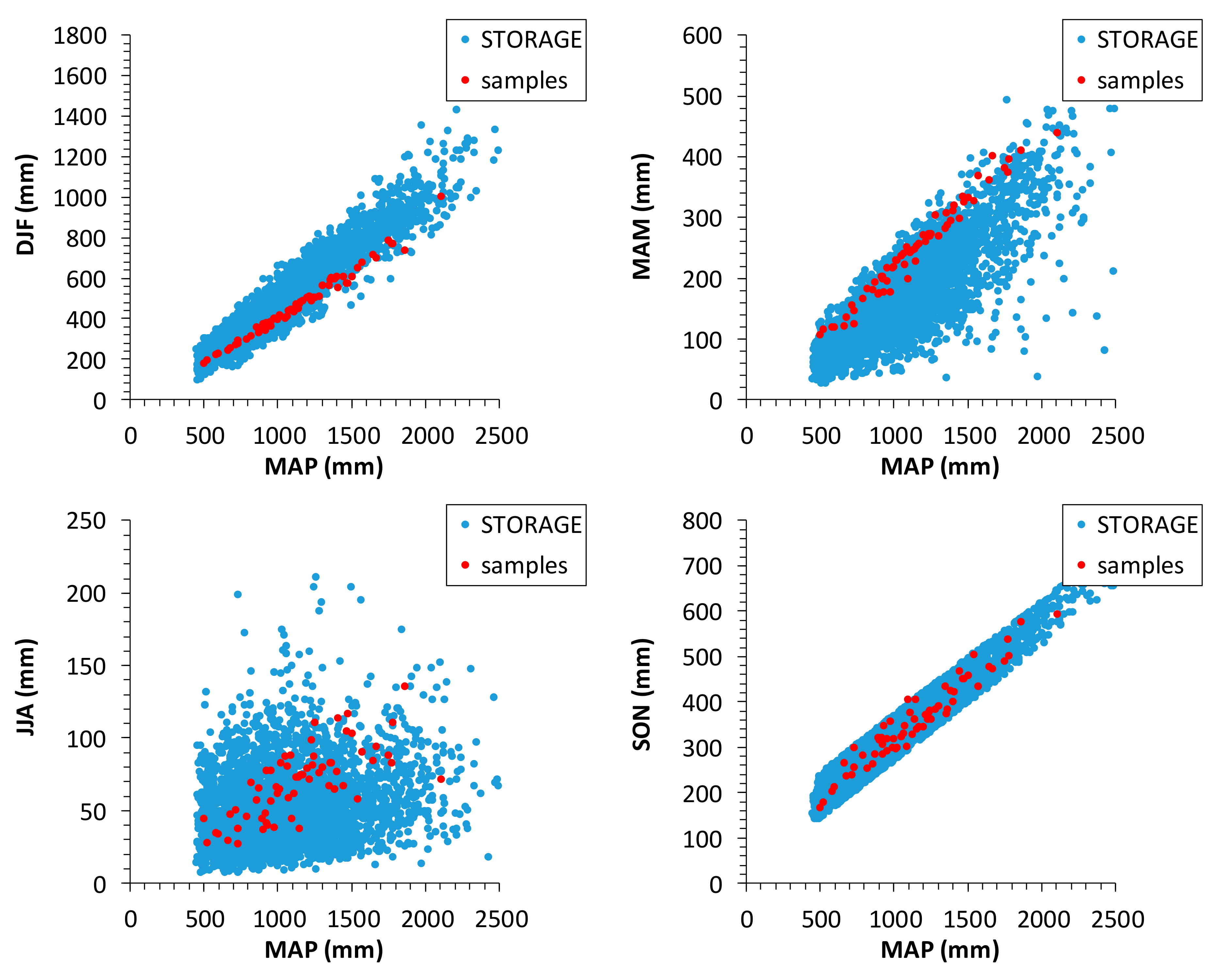
  • mean values for seasonal rainfall in DJF (December–January–February), MAM (March–April–May), JJA (June–July–August), and SON (September–October–November).
The results of this composite filter, constituted by a subset of 50,000 parametric sets, are illustrated in Section 4 for the Calabria region. The storage of this information further justifies the choice of the acronym STORAGE. In fact, the software allows to use, for the synthetic generation related to a single rain gauge of interest, parametric sets belonging to this pre-existing “information reservoir” (regarding a wide previously investigated area), for which the corresponding series of AMR, annual rainfall, seasonal rainfall and number of wet days are comparable with those related to the sample historical data. Obviously, this aspect considerably reduces the calculation times for the model calibration on a specific site of interest, with respect to a usual calibration procedure that is carried out without any a priori indication about possible model outcomes. It is clear that this “information reservoir” can be continuously updated when other areas are investigated as case studies. Moreover, refinement algorithms will be implemented in future versions of STORAGE, in order to enhance the performance of calibration for a specific rain gauge.
Table 1. Ranges of variation for parameters in STORAGE, according to [7,54].
ParameterMinMax
1 / λ 0 (days)530
θ 0 (-)220
1 / β W (h)524
1 / β I , 0 (mm/h)520
1 / β D , 0 (h)0.10.6
1 / λ min (days)0.55
θ min (-)12
ϕ 1 , λ (rad)0π/2
χ (-)0.51
η (-)0.51
ξ (-)01
ϕ 2 , λ (rad)0

3.2. The User-Friendly Interface of STORAGE

When a user executes STORAGE, after having enabled the VBA macros, the Main worksheet will appear as in Figure 3. Two different procedures are allowed for the generation of a synthetic rainfall time series, and each one is associated with a specific command button:
  • RUN with parameter values chosen by the user;
  • PARAMETER ESTIMATION AND RUN.
Moreover, in the Main worksheet, the user can manually stop the elaborations in progress with the related command button (manual STOP to elaborations).
Figure 3. Interface of the Main worksheet of STORAGE after enabling the VBA macros’ content.
Hydrology 08 00076 g003
In addition to the Main worksheet, STORAGE contains the following worksheets:
  • Annual and Monthly Rainfall, in which the generated rainfall values, aggregated at monthly and annual timescale, as well as the annual number of wet days, will be printed (for each generated year);
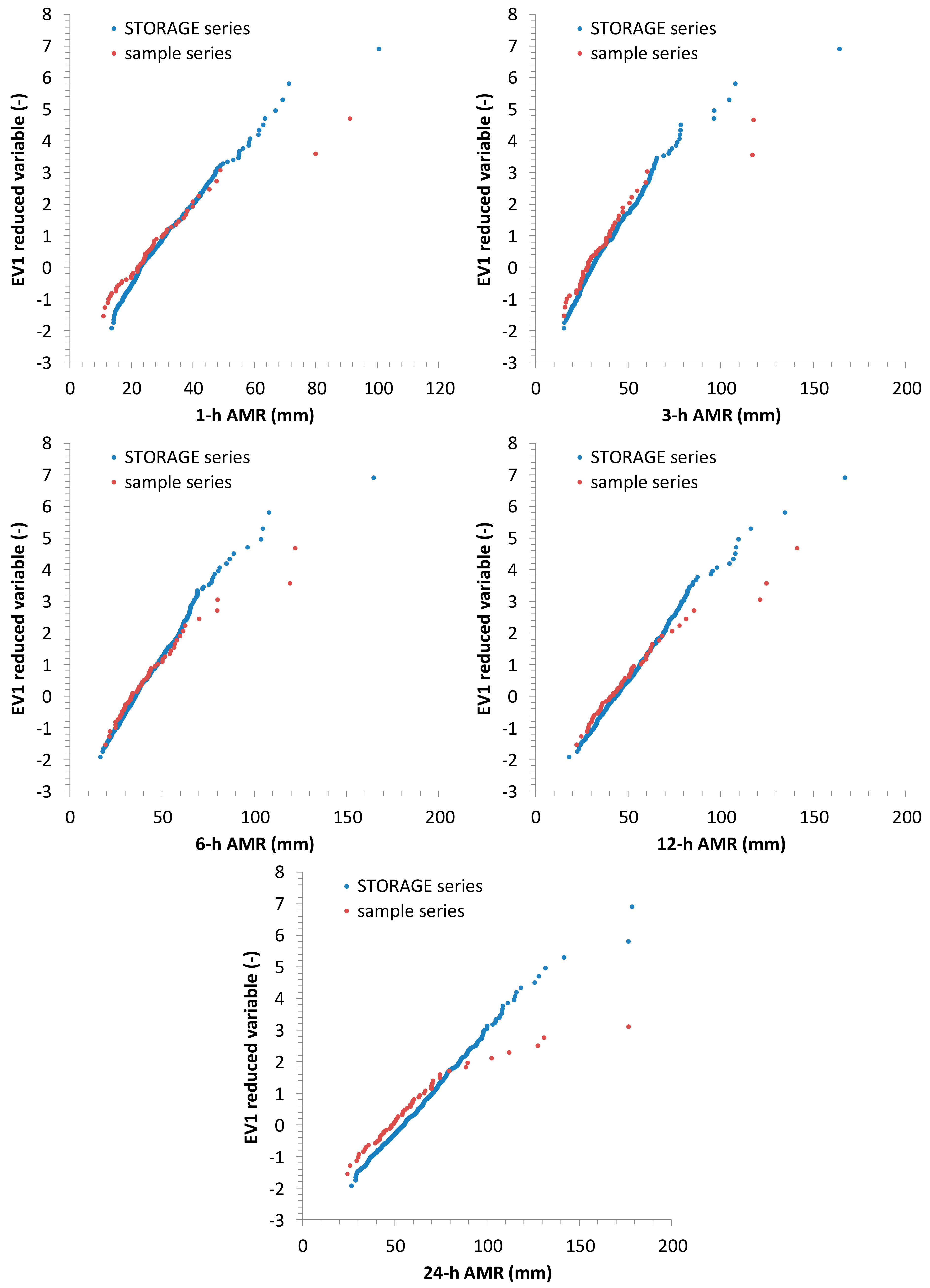
  • Annual Maxima, where the values for AMR series will be printed for rainfall durations equal to 5, 15, 30, 60 min, 3, 6, 12, 24 h, and 1 day;
  • Statistics, in which the mean and standard deviation values will be calculated and printed for all the quantities reported in the previous points 1 and 2;
  • EV1 Plots, in which the frequency distributions of all the previously listed AMR series will be represented on EV1 (Extreme Values type 1) probabilistic plots;
  • Average Monthly Rainfall Plot, which contains the histogram of the average monthly rainfall values related to the generated rainfall series;
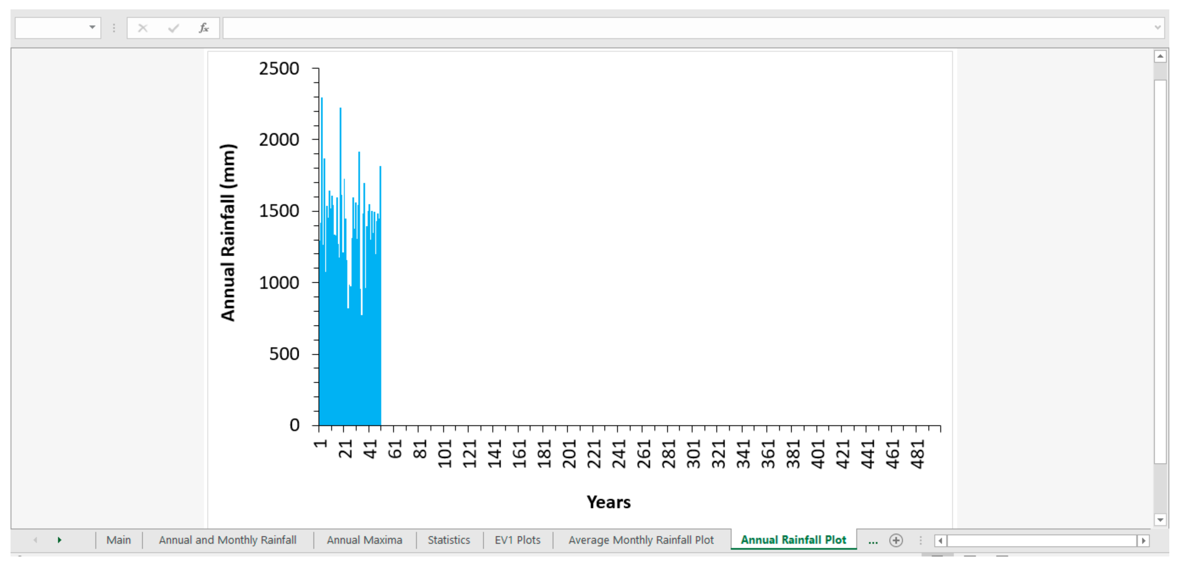
  • Annual Rainfall Plot, where the annual cumulative rainfall series is represented.
Concerning the Annual Maxima worksheet, the series from 60 min to 24 h are estimated by considering the continuous series with a time step of 1 h. This choice is justified by the fact that many observed AMR series around the world were extracted, until 20–30 years ago, by using 1-h continuous data, while data with resolutions lower than 1 h are available only from 1990 or later [55]. Consequently, the comparison among synthetic and observed AMR series should be preferred by using this setting.

3.2.1. Data Input

For both previously mentioned procedures of time series generation, it is necessary to insert the following input information before starting the elaborations:
  • the number of years to be generated (Cell D3). The maximum allowed is 500 years;
  • the time resolution, expressed in minutes (Cell D4). The software allows for resolutions of 1, 5, 10, 15, 20, 30 and 60 min.
If the option RUN with parameter values chosen by the user is selected, then the user has to fill all the cells from C10 to C22 (Figure 3).
On the contrary, if PARAMETER ESTIMATION AND RUN is chosen, then the user has to insert the following input data, which are sample estimates from the observed series of the investigated case study:
  • The values of parameters for Amount–Duration–Frequency (ADF) curves, expressed as a power function:
    h T d = a T d n T
    where d is the rainfall duration (hours) ranging from 1 to 24 h, T is the return period (years), h T d is the d-AMR associated with T, and a T and n T are ADF parameters. In detail, the values for a T and n T , associated with specific T values, are requested:
    concerning a T , the cells to be filled are F5 (T = 2 years), H5 (T = 5 years), J5 (T = 10 years), F8 (T = 50 years), H8 (T = 100 years) and J8 (T = 200 years);
    concerning n T , the cells to be filled are G5 (T = 2 years), I5 (T = 5 years), K5 (T = 10 years), G8 (T = 50 years), I8 (T = 100 years) and K8 (T = 200 years).
    If the size of the sample AMR series for the investigated case study is limited (less than 20 years), then it is advisable to use only sample estimates from low T values (2, 5 and 10 years). For higher sample sizes, information deriving from higher return periods can also be entered.
  • The values for Mean Annual Precipitation (MAP) into the cell L5, for the mean annual number of wet days into the cell M5, and for the mean cumulative seasonal precipitation, associated with December–January–February (DJF), March–April–May (MAM), June–July–August (JJA) and September–October–November (SON), into the cells L8, M8, N8 and O8, respectively. Moreover, also in this case, it not necessary to fill all the listed cells. The VBA macro will run the model calibration on the basis of the available information. Concerning the cell M5, strictly related to the wet day proportion, it should be remarked that the trivial rainfall (of which amount is less than the capacity of the tipping bucket of the rain gauges) could highly distort the result of the calibration in some cases, and so not filling this cell could avoid this possibility.
An example of Data Input is shown in Figure 4, if the option PARAMETER ESTIMATION AND RUN is selected by the user.

3.2.2. Synthetic Generation of Rainfall Time Series at a High Resolution

After completing the Data Input step, it is possible to run one of the two generation procedures. In the following pages, attention is focused on the PARAMETRIC ESTIMATION AND RUN button (Figure 4), which further allows for different generation alternatives. The table and graphic outputs, associated to RUN with parameter values chosen by the user button (Section 3.2.4), are similar.
It must be highlighted that, in a worksheet hidden for the user, the results deriving from the use of about 3500 parametric sets, in terms of a T and n T for the ADF, MAP and the mean annual number of wet days, and mean cumulative seasonal rainfalls (DJF, MAM, JJA, SON), are stored. In detail (see also Section 3.1.2 and Section 4), for each single parametric set, 200 years of precipitation were synthetically generated.
By clicking on the PARAMETRIC ESTIMATION AND RUN button, the userform shown in Figure 5 is displayed; from the combobox at the top (Figure 6) it is possible to select the statistical descriptors to be reproduced, i.e.,:
  • only the parameters a T and n T of the ADF curves;
  • only MAP and the mean value for annual number of wet days (NumWetDays);
  • a T , n T , MAP and NumWetDays;
  • a T , n T , MAP, NumWetDays and the mean cumulative seasonal rainfalls (DJF, MAM, JJA, SON).
After the choice of the descriptors to be reproduced (for example, a T , n T , MAP, NumWetDays, DJF, MAM, JJA, and SON, as in Figure 6), it is possible to click on the PARAMETRIC ESTIMATION button. The software will display by default, in the cell range C10:C22, the parametric set (indicated with ID SET 1) which is characterized, among the 3500 used offline, by the best value (i.e., the lowest value) of the evaluated Objective Function (OF) (Figure 7), in percentage terms, as:
O F = O F   a _ n O p t i o n    1 O F   M A P _ N u m W e t D a y s O p t i o n    2 O F   a _ n + O F   M A P _ N u m W e t D a y s O p t i o n    3 O F   a _ n + O F   M A P _ N u m W e t D a y s + O F   S e a s o n s O p t i o n    4
in which:
O F   a _ n = i = 1 K a a i a i * a i + j = 1 K n n j n j * n j
where:
a i is the i-th value (i = 1, … K a ) of parameter a for an ADF curve of an assigned T, inserted by the user into an input cell, while a i * is the correspondent NSRP value. K a is the number of return periods T which are considered by the user for parameter a.
n j is the j-th value (j = 1, … K n ) of parameter n for an ADF curve of an assigned T, inserted by the user into an input cell, while n j * is the correspondent NSRP value. K n is the number of return periods T which are considered by the user for parameter n.
O F   M A P _ N u m W e t D a y s = = M A P M A P * M A P + N u m W e t D a y s N u m W e t D a y s * N u m W e t D a y s
where M A P and N u m W e t D a y s are the sample values which are inserted by the user, while M A P * e N u m W e t D a y s * are the correspondent NSRP values.
O F   S e a s o n s = D J F D J F * D J F + M A M M A M * M A M + J J A J J A * J J A + S O N S O N * S O N
where D J F , M A M , J J A and S O N are the sample values which are inserted by the user, while D J F * , M A M * , J J A * and S O N * are the correspondent NSRP values.
Whatever option is selected in the combobox, STORAGE will provide the correspondent values for all the OFs (Equations (13)–(15)) for a specific parameter set.
Moreover, by using the spin button (Figure 8), it is possible to adopt other parameter sets for simulation, which are sorted (by STORAGE in the hidden worksheet) on the basis of the values related to the selected OF.
After the choice for parametric set, the user can click on the RUN button for carrying out the generation of a synthetic rainfall series.
During the run, the user can control the progress of generation by analyzing the several worksheets in STORAGE.xlsm. As examples, the cell D5 in Main (Figure 9) and the histogram for Annual Rainfall (Figure 10) can be checked.
A message box will appear when simulation is completed. Then, the final results can be analyzed in the several tables and plots of STORAGE (Figure 11), while the whole synthetic rainfall series at the selected high resolution (cell D4 in Main), will be printed in “C:\NSRP\RainSim.txt”.
As explained in the following sections, STORAGE also allows for rainfall generation with multisets approaches, as an alternative way to the run with a single parametric set.
Figure 5. Userform where a user can carry out calibration and select several run options.
Hydrology 08 00076 g005
Figure 6. Example of procedure for calibration, by using the combobox at the top of the userform.
Hydrology 08 00076 g006
Figure 7. Example of calibration results in the Main worksheet.
Hydrology 08 00076 g007
Figure 8. Example of calibration by using the spin button, which allows for using other parameter sets for simulation.
Hydrology 08 00076 g008
Figure 9. During the run, the user can control the progress of generation by checking the number of simulated years in the cell D5 in the Main worksheet.
Hydrology 08 00076 g009
Figure 10. During the run, the user can control the progress of generation by analyzing the histogram for Annual Rainfall.
Hydrology 08 00076 g010
Figure 11. Examples of visualization in the different worksheets when the simulations are completed.
Hydrology 08 00076 g011

3.2.3. Multisets Approaches

Focusing on Option 4 of Equation (12), different parametric sets can be characterized by very similar OF values among them, but some sets could better reconstruct ADF curves, while other ones could best fit MAP and NumWetDays, and so on.
In this context, if the fourth option of Equation (12) (i.e., a T , n T , MAP, NumWetDays, DJF, MAM, JJA, SON) is chosen as an ensemble of statistical descriptors to be reproduced, the user can take advantages from several parametric sets by selecting one of these two options concerning multisets approaches (Figure 12):
  • Ranking from total OF;
  • Merging different OFs, which is further subdivided in 3 OFs and 4 OFs.
The proposed multisets approaches are based on the concept of equifinality [56], which means that “different parametric sets within a chosen model structure may be behavioural or acceptable in reproducing the observed behaviour of that system”.

Ranking from Total OF

It is possible to select S parametric sets (sorted with increasing values of Option 4 in Equation (12)) by using the spin button of Figure 12.
Figure 12. Example of multisets approach regarding the option “Ranking from total OF”.
Hydrology 08 00076 g012
Automatically, STORAGE will assign (to a specific set) a frequency of use which is inversely proportional to its overall OF value (Option 4 in Equation (12)). In detail, let f i be the frequency of use for the i-th parametric set (i = 1, …, S) and O F i its corresponding value of OF; f i is computed as:
f i = 1 O F i i = 1 S 1 O F i
with, obviously, i = 1 S f i = 1 .
Then, considering the total number N of years to simulate (input data in cell D3 in the Main worksheet, Figure 4), the number f i N of years will be generated with the i-th parametric set.
It should be highlighted that:
  • if a multisets approach is selected, a user should consider at most S = 4 and a large value for N (we suggest N = 500 years), in order to have a significant number of years for each set (with N = 500 years and S = 4, there are on average 125 years which are simulated with each set);
  • in a context, such as in this case, of stationary/cycle-stationary process (i.e., without any climatic trend), it is not necessary to generate a large number L of N-year synthetic series (in which each i-th set should regard f i L series), but it is sufficient to consider the generation of only one year, which is repeated L = N times. This is allowed by the ergodicity property of a stationary process [57], which means that the statistics from a long temporal N-year series are equal to the statistics from one year (generated N times).
After clicking on the RUN command button (Figure 12), the user is able to check the progress of the rainfall generation, similarly to the procedure with only one parameter set (Figure 9, Figure 10 and Figure 11). It is clear that this approach can be well used for a more comprehensive sensitivity analysis (i.e., not only related for the first ranked parametric sets) in further upgraded versions of STORAGE software.

Merging Different OFs

This approach can be carried out in two options:
  • 3 OFs;
  • 4 OFs.
In the first case, from the worksheet (hidden for the user) where the information of the offline generations with about 3500 parametric sets is stored, the VBA code selects the three parametric sets with the lowest values for, respectively, Equations (13)–(15). Then, STORAGE will assign to each selected set a frequency f i , evaluated by considering Option 4 of Equation (12) as O F i in Equation (16).
In the second case (4 OFs), the parametric set with the lowest value of the overall OF (option 4 of Equation (12)) is also considered, together with the three above mentioned sets.
It must be highlighted that these two options are allowed by STORAGE only if all the 3 OFs of the first option are inside the first 10 positions of the ranking for OF calculated with Option 4 of Equation (12).
Also in this case, after clicking on the 3 OFs or 4 OFs buttons (Figure 13), the user is able to check the progress of the rainfall generation, similarly to the procedures with only one parameter set (Figure 9, Figure 10 and Figure 11).

3.2.4. RUN with Parameter Values Chosen by the User

This option allows for manually setting the values for the parameters in the interval C10:C21 of cells in the Main worksheet (Figure 4). Also in this case, after clicking on the corresponding command button for the run, the user is able to check the progress of the rainfall generation, similar to the previous described procedures. The ranges of variation for parameters are reported in Table 1, according to [7,54].

4. Application for Rain Gauge Network of the Calabria Region and Discussion

As regards the application for the Calabria region, we saved in STORAGE about 3500 parametric sets, for which the 200-year synthetic series presented summary statistics ranging inside specific intervals (according to the observed data in the whole region). In detail:
  • concerning MAP, a value between 450 and 2500 mm;
  • concerning the mean annual number of wet days, a value between 50 and 120;
  • concerning the ADF curves (Equation (11)), values of a and n for T = 5 years between 20 and 65 mm/h and between 0.12 and 0.65, respectively;
  • concerning the SON cumulative rainfall, a mean value inside a variation of ±50 mm with respect to the linear regression curve between observed MAP and SON of the investigated data series.
By applying this composite filter, graphical comparisons among synthetic and observed summary statistics are shown in Figure 14 and Figure 15. From analysis of these dispersion plots, the STORAGE good reconstruction for the investigated rainfall descriptors can be assessed.
For the sake of brevity, focusing on specific rain gauge data series, examples of STORAGE application are below described for Montalto Uffugo, Reggio Calabria and Vibo Valentia stations. Their associated sample values for the statistical descriptors are reported in Table 2 and Table 3.
For all the three stations, 500-year synthetic rainfall time series with a resolution of 5 min were generated, and we carried out model validation by analyzing the reproduction of frequency distributions for sample data of AMR, annual and seasonal rainfall, and annual number of wet days. The best STORAGE performances were obtained:
  • by using the parametric set with the lowest value for the total OF (Option 4 in Equation (12)), concerning Montalto Uffugo;
  • by considering the multisets approach Ranking from total OF for Reggio Calabria and Vibo Valentia, with S equal to 3 and 4, respectively.
For Montanto Uffugo rain gauge, STORAGE provided a 500-year synthetic rainfall time series which satisfactorily reproduces the frequency distributions of AMR sample data (see the EV1 probabilistic plots in Figure 16), with an over-estimation only for 24-h AMR series. The reproduction of the frequency distributions concerning sample series for annual rainfall, annual number of wet days, and seasonal precipitation in DJF, MAM and SON is analyzed on Gaussian plots (Figure 17): a slight underestimation is obtained only for JJA rainfall. As regards Reggio Calabria and Vibo Valentia rain gauges, the obtained results (Figure 18, Figure 19, Figure 20 and Figure 21) highlighted some crucial aspects to be investigated further when future developments in STORAGE software will be carried out. In detail:
  • when AMR sample data present outliers from an EV1 behaviour (Figure 18 and Figure 20), or if extremes are underestimated, it could be useful to consider other probability distributions for cell intensity I (e.g., Weibull, Gamma or a mixture of exponential functions, [20,25,58]), and/or to use other shapes for rain cells (such as the sinusoidal one, [59]), in order to better reproduce quantiles at high values of return period T;
  • though frequency distributions of annual rainfall are properly reproduced, an increase in the maximum number of harmonics for 1 / λ (i.e., the mean inter-arrival time between two consecutive storms) and/or modelling seasonality also for 1 / β W (i.e., the mean waiting time between a specific burst origin and the origin of the associated storm) could improve the reconstruction of both the annual number of wet days and seasonal rainfall in some specific cases.
Starting from this latter aspect, a more in-depth investigation of the maximum number of harmonics for some quantities, and of their phase shifts, could justify the STORAGE application also in regions far from the investigated area, i.e., characterized by drier or wetter climates. This obviously means to increase the number of parametric sets to be stored in the software.
Further analyses of STORAGE performances were carried out focusing on Montalto Uffugo rain gauge, characterized by 30-year continuous time series at resolutions of 20 min. Such analyses aim to evaluate the model capacity for reproducing summary statistics of high-resolution continuous series (not used for STORAGE calibration) and to compare the STORAGE results with those from a standard NSRP (i.e., calibrated by only using continuous high-resolution data). In details:
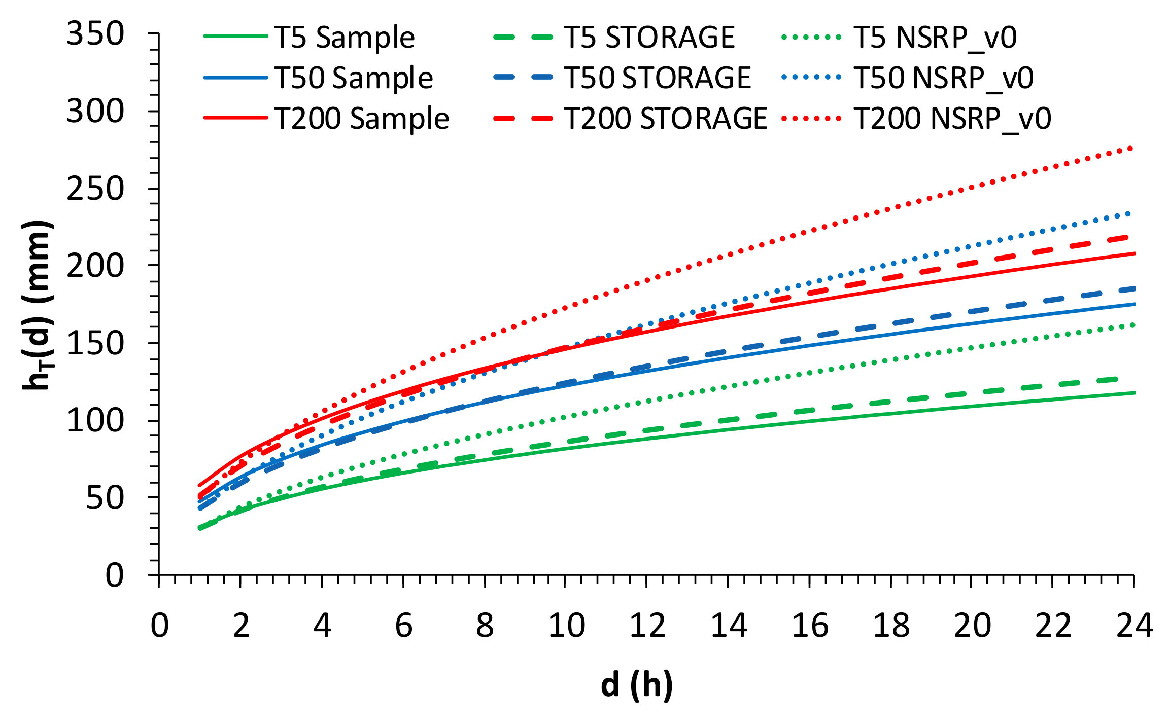
  • we calibrated a basic version of NSRP with the 1-h continuous data series (aggregated from the available 20-min one), by estimating parameters for each month (according to [14]) in order to avoid possible underestimation of extremes (as mentioned in the introduction). This version of NSRP is indicated as NSRP_v0 in the following;
  • we compared STORAGE and NSRP_v0 performances, graphically and in terms of Root Mean Square Error (RMSE), as regards the modelling of:
    mean, standard deviation and percentage of dry intervals from the continuous series at 20-min and 1-h resolutions;
    mean values of monthly rainfall heights;
    rainfall heights of ADF curves for return periods T = 5, 50 and 200 years.
Concerning the summary statistics of the continuous series, it is clear that NSRP_v0 provides the best performances for 1-h resolution, because this time step was used for NSRP calibration in this case. However, the obtained STORAGE results for 1-h data series can be considered acceptable for the mean and percentage of dry intervals (Table 4 and Figure 22). For a 20-min resolution, STORAGE and NSRP_v0 performances are comparable (Table 4 and Figure 23).
Moreover, monthly rainfall heights are very well reproduced by STORAGE, as seasonal rainfalls are used for its calibration (Section 3.2.1 and Section 3.2.2), but NSRP_v0 results can be also considered good: RMSE values are 7.5 and 14.4 mm for STORAGE and NSRP_v0, respectively (see Table 5 and Figure 24).
The clear benefit of using STORAGE is highlighted by focusing on ADF curves (Table 5 and Figure 25). As expected, STORAGE provides a very good reconstruction (RMSE values are comprised between 5.5 and 6 mm) because it is calibrated with a T and n T of the sample ADF curves (Section 3.2.1 and Section 3.2.2). On the contrary, NSRP_v0 significantly overestimates rainfall extremes in this specific case; as its parametric estimation is only based on summary statistics from high-resolution continuous series, an acceptable reproduction of ADF curves could not be guaranteed in general (such as for Montalto Uffugo rain gauge), also by using monthly or seasonal parameter sets.
This last comparison allows us to remark the most important aspect of the usefulness of STORAGE, i.e., the possibility of calibrating an SRG by only using information at coarser resolutions (AMR, MAP, and so on) and then generating continuous series which preserves sample features (often un-known for lack of data) in an acceptable way at high resolutions.
Figure 16. Montalto Uffugo rain gauge: EV1 probabilistic plots, showing the comparison among synthetic and observed AMR series.
Hydrology 08 00076 g016
Figure 17. Montalto Uffugo rain gauge: Gaussian probabilistic plots, showing the comparison among synthetic and observed series, regarding annual and seasonal rainfall, and annual number of wet days.
Hydrology 08 00076 g017
Figure 18. Reggio Calabria rain gauge: EV1 probabilistic plots, showing the comparison among synthetic and observed AMR series.
Hydrology 08 00076 g018
Figure 19. Reggio Calabria rain gauge: Gaussian probabilistic plots, showing the comparison among synthetic and observed series, regarding annual and seasonal rainfall, and annual number of wet days.
Hydrology 08 00076 g019
Figure 20. Vibo Valentia rain gauge: EV1 probabilistic plots, showing the comparison among synthetic and observed AMR series.
Hydrology 08 00076 g020
Figure 21. Vibo Valentia rain gauge: Gaussian probabilistic plots, showing the comparison among synthetic and observed series, regarding annual and seasonal rainfall, and annual number of wet days.
Hydrology 08 00076 g021
Figure 22. Montalto Uffugo rain gauge: comparison between STORAGE and NSRP_v0 performances, focusing on the mean, standard deviation and percentage of dry intervals for the continuous 1-h series.
Hydrology 08 00076 g022
Figure 23. Montalto Uffugo rain gauge: comparison between STORAGE and NSRP_v0 performances, focusing on the mean, standard deviation and percentage of dry intervals for the continuous 20-min series.
Hydrology 08 00076 g023
Figure 24. Montalto Uffugo rain gauge: comparison between STORAGE and NSRP_v0 performances, focusing on mean values of monthly rainfall heights.
Hydrology 08 00076 g024
Figure 25. Montalto Uffugo rain gauge: comparison between STORAGE and NSRP_v0 performances, focusing on ADF curves.
Hydrology 08 00076 g025

5. Conclusions

The developed STORAGE software constitutes a very useful user-friendly tool for generating long rainfall time series at high resolutions, which could be applied as input data in many hydrological analyses, such as in the continuous rainfall-runoff modeling.
The innovative aspects of the software regard: (i) the possibility of using information, for model calibration, from observed time series which are longer than continuous data sample at high resolutions; (ii) the modelling of seasonality by adopting goniometric series, which allows for a more parsimonious approach with respect to considering monthly parametric sets (as is usually done).
The presented version of STORAGE software, available at https://sites.google.com/unical.it/storage, is currently suitable for the reproduction of rainfall series which exhibit a clear EV1 behaviour in terms of AMR and present values of annual and seasonal precipitation that are typical of the Mediterranean area.
Future developments will concern: (i) the extension of the ensemble of the parametric sets and the possibility to use other probability distributions for some rainfall features and other shapes besides the rectangular one for rain cells, in order to apply the model in other regions with different climates with respect to the investigated area; (ii) the implementation of a module for obtaining perturbed synthetic series, which can be representative of future hypothesized rainfall scenarios on spatial and temporal hydrological scales.
Moreover, the authors consider as very important the possibility of implementing in STORAGE specific modules related to soft computing methods (widely used in recent literature [60,61,62]), in order to provide different approaches for a specific case study. This aspect will allow to immediately compare the performances of an SRG (having a mathematical structure which is “physically-based”, as it models some aspects of rainfall genesis, see Figure 2) with those from approaches such as Artificial Neural Networks (ANNs), Support Vector Regression (SVR) and Fuzzy Logic (FL), which are characterized by high nonlinearity, flexibility and data-driven learning.

Author Contributions

Conceptualization, D.L.D.L. and A.P.; methodology, D.L.D.L. and A.P.; software, D.L.D.L.; validation, D.L.D.L. and A.P.; data curation, D.L.D.L.; writing—original draft preparation, D.L.D.L. and A.P.; writing—review and editing, D.L.D.L. and A.P. All authors have read and agreed to the published version of the manuscript.

Funding

This research received no external funding.

Institutional Review Board Statement

Not applicable.

Informed Consent Statement

Not applicable.

Acknowledgments

This work was supported by the Italian Ministry for Ecological Transition (Ministero della Transizione Ecologica—Direzione Generale per la sicurezza del suolo e dell’Acqua-SUA), through the Law 5/1/2017 n. 4 “Interventi per il sostegno della formazione e della ricerca nelle scienze geologiche, per progetti di ricerca finalizzati alla previsione e alla prevenzione dei rischi geologici”.

Conflicts of Interest

The authors declare no conflict of interest.

References

  1. Grimaldi, S.; Nardi, F.; Piscopia, R.; Petroselli, A.; Apollonio, C. Continuous hydrologic modelling for design simulation in small and ungauged basins: A step forward and some tests for its practical use. J. Hydrol. 2020, 595, 125664. [Google Scholar] [CrossRef]
  2. Młyński, D.; Wałęga, A.; Petroselli, A.; Tauro, F.; Cebulska, M. Estimating Maximum Daily Precipitation in the Upper Vistula Basin, Poland. Atmosphere 2019, 10, 43. [Google Scholar] [CrossRef] [Green Version]
  3. Onof, C.; Chandler, R.E.; Kakou, A.; Northrop, P.; Wheater, H.S.; Isham, V. Rainfall modelling using Poisson-cluster processes: A review of developments. Stoch. Environ. Res. Risk Assess. 2000, 14, 384–411. [Google Scholar] [CrossRef]
  4. Wheater, H.S.; Chandler, R.E.; Onof, C.J.; Isham, V.S.; Bellone, E.; Yang, C.; Lekkas, D.; Lourmas, G.; Segond, M.-L. Spatial-temporal rainfall modelling for flood risk estimation. Stoch. Environ. Res. Risk Assess. 2005, 19, 403–416. [Google Scholar] [CrossRef]
  5. Ritschel, C.; Ulbrich, U.; Névir, P.; Rust, H.W. Precipitation extremes on multiple timescales—Bartlett–Lewis rectangular pulse model and intensity–duration–frequency curves. Hydrol. Earth Syst. Sci. 2017, 21, 6501–6517. [Google Scholar] [CrossRef] [Green Version]
  6. De Luca, D.L.; Petroselli, A.; Galasso, L. Modelling Climate Changes with Stationary Models: Is It Possible or Is It a Paradox? In Numerical Computations: Theory and Algorithms; NUMTA 2019. Lecture Notes in Computer Science; Sergeyev, Y., Kvasov, D., Eds.; Springer Science and Business Media LLC: Berlin/Heidelberg, Germany, 2020; Volume 11974, pp. 84–96. [Google Scholar]
  7. De Luca, D.; Petroselli, A.; Galasso, L. A Transient Stochastic Rainfall Generator for Climate Changes Analysis at Hydrological Scales in Central Italy. Atmosphere 2020, 11, 1292. [Google Scholar] [CrossRef]
  8. Willems, P.; Arnbjerg-Nielsen, K.; Olsson, J.; Nguyen, V. Climate change impact assessment on urban rainfall extremes and urban drainage: Methods and shortcomings. Atmospheric Res. 2012, 103, 106–118. [Google Scholar] [CrossRef]
  9. Maraun, D. Bias Correcting Climate Change Simulations—A Critical Review. Curr. Clim. Chang. Rep. 2016, 2, 211–220. [Google Scholar] [CrossRef] [Green Version]
  10. Kendon, E.J.; Roberts, N.M.; Fowler, H.J.; Roberts, M.J.; Chan, S.C.; Senior, C.A. Heavier summer downpours with climate change revealed by weather forecast resolution model. Nat. Clim. Chang. 2014, 4, 570–576. [Google Scholar] [CrossRef] [Green Version]
  11. Ban, N.; Schmidli, J.; Schär, C. Heavy precipitation in a changing climate: Does short-term summer precipitation increase faster? Geophys. Res. Lett. 2015, 42, 1165–1172. [Google Scholar] [CrossRef]
  12. Cameron, D.; Beven, K.; Tawn, J. An evaluation of three stochastic rainfall models. J. Hydrol. 2000, 228, 130–149. [Google Scholar] [CrossRef]
  13. Cowpertwait, P.S.P. Further developments of the neyman-scott clustered point process for modeling rainfall. Water Resour. Res. 1991, 27, 1431–1438. [Google Scholar] [CrossRef]
  14. Cowpertwait, P.; O’Connell, P.; Metcalfe, A.; Mawdsley, J. Stochastic point process modelling of rainfall. I. Single-site fitting and validation. J. Hydrol. 1996, 175, 17–46. [Google Scholar] [CrossRef]
  15. Cowpertwait, P.; Isham, V.; Onof, C. Point process models of rainfall: Developments for fine-scale structure. Proc. R. Soc. A Math. Phys. Eng. Sci. 2007, 463, 2569–2587. [Google Scholar] [CrossRef]
  16. Entekhabi, D.; Rodriguez-Iturbe, I.; Eagleson, P.S. Probabilistic representation of the temporal rainfall process by a modified Neyman-Scott Rectangular Pulses Model: Parameter estimation and validation. Water Resour. Res. 1989, 25, 295–302. [Google Scholar] [CrossRef] [Green Version]
  17. Gyasi-Agyei, Y. Identification of regional parameters of a stochastic model for rainfall disaggregation. J. Hydrol. 1999, 223, 148–163. [Google Scholar] [CrossRef]
  18. Gyasi-Agyei, Y.; Willgoose, G.R. A hybrid model for point rainfall modeling. Water Resour. Res. 1997, 33, 1699–1706. [Google Scholar] [CrossRef]
  19. Islam, S.; Entekhabi, D.; Bras, R.L.; Rodriguez-Iturbe, I. Parameter estimation and sensitivity analysis for the modified Bartlett-Lewis rectangular pulses model of rainfall. J. Geophys. Res. Space Phys. 1990, 95, 2093–2100. [Google Scholar] [CrossRef]
  20. Kaczmarska, J.; Isham, V.; Onof, C. Point process models for fine-resolution rainfall. Hydrol. Sci. J. 2014, 59, 1972–1991. [Google Scholar] [CrossRef] [Green Version]
  21. Khaliq, M.; Cunnane, C. Modelling point rainfall occurrences with the modified Bartlett-Lewis rectangular pulses model. J. Hydrol. 1996, 180, 109–138. [Google Scholar] [CrossRef]
  22. Kim, D.; Olivera, F.; Cho, H.; Socolofsky, S.A. Regionalization of the Modified Bartlett-Lewis Rectangular Pulse Stochastic Rainfall Model. Terr. Atmos. Ocean. Sci. 2013, 24, 421–436. [Google Scholar] [CrossRef] [Green Version]
  23. Kim, D.; Kwon, H.-H.; Lee, S.-O.; Kim, S. Regionalization of the Modified Bartlett–Lewis rectangular pulse stochastic rainfall model across the Korean Peninsula. HydroResearch 2016, 11, 123–137. [Google Scholar] [CrossRef]
  24. Kim, D.; Cho, H.; Onof, C.; Choi, M. Let-It-Rain: A web application for stochastic point rainfall generation at ungaged basins and its applicability in runoff and flood modeling. Stoch. Environ. Res. Risk Assess. 2017, 31, 1023–1043. [Google Scholar] [CrossRef] [Green Version]
  25. Kim, D.; Onof, C. A stochastic rainfall model that can reproduce important rainfall properties across the timescales from sev-eral minutes to a decade. J. Hydrol. 2020, 589, 125150. [Google Scholar] [CrossRef]
  26. Kossieris, P.; Efstratiadis, A.; Koutsoyiannis, D. Coupling the strengths of optimization and simulation for calibrating Poisson cluster models. In Proceedings of the Facets of Uncertainty: 5th EGU Leonardo Conference–Hydrofractals 2013–STAHY 2013, Kos Island, Greece, 17–19 October 2013. [Google Scholar]
  27. Onof, C.; Wheater, H.S. Improved fitting of the Bartlett-Lewis Rectangular Pulse Model for hourly rainfall. Hydrol. Sci. J. 1994, 39, 663–680. [Google Scholar] [CrossRef]
  28. Onof, C.; Wheater, H.S. Improvements to the modelling of British rainfall using a modified Random Parameter Bartlett-Lewis Rectangular Pulse Model. J. Hydrol. 1994, 157, 177–195. [Google Scholar] [CrossRef]
  29. Paschalis, A.; Molnar, P.; Fatichi, S.; Burlando, P. On temporal stochastic modeling of precipitation, nesting models across scales. Adv. Water Resour. 2014, 63, 152–166. [Google Scholar] [CrossRef]
  30. Smithers, J.; Pegram, G.; Schulze, R. Design rainfall estimation in South Africa using Bartlett–Lewis rectangular pulse rainfall models. J. Hydrol. 2002, 258, 83–99. [Google Scholar] [CrossRef]
  31. Velghe, T.; Troch, P.A.; De Troch, F.P.; Van De Velde, J. Evaluation of cluster-based rectangular pulses point process models for rainfall. Water Resour. Res. 1994, 30, 2847–2857. [Google Scholar] [CrossRef]
  32. Verhoest, N.; Troch, P.A.; De Troch, F.P. On the applicability of Bartlett–Lewis rectangular pulses models in the modeling of design storms at a point. J. Hydrol. 1997, 202, 108–120. [Google Scholar] [CrossRef]
  33. Wasko, C.; Pui, A.; Sharma, A.; Mehrotra, R.; Jeremiah, E. Representing low-frequency variability in continuous rainfall simulations: A hierarchical random Bartlett Lewis continuous rainfall generation model. Water Resour. Res. 2015, 51, 9995–10007. [Google Scholar] [CrossRef] [Green Version]
  34. Wheater, H.S.; Isham, V.S.; Chandler, R.E.; Onof, C.J.; Stewart, E.J. Improved Methods for National Spatial–Temporal Rainfall and Evaporation Modelling for BSM; Department for Environment, Food and Rural Affairs (DEFRA); Flood Management Division: London, UK, 2007. [Google Scholar]
  35. Verhoest, N.; Vandenberghe, S.; Cabus, P.; Onof, C.; MecaFigueras, T.; Jameleddine, S. Are stochastic point rainfall models able to preserve extreme flood statistics? Hydrol. Process. 2010, 24, 3439–3445. [Google Scholar] [CrossRef] [Green Version]
  36. Cowpertwait, P.S.P. A generalized point process model for rainfall. Proc. R. Soc. Lond. Ser. A Math. Phys. Sci. 1994, 447, 23–37. [Google Scholar] [CrossRef]
  37. Cameron, D.; Beven, K.; Tawn, J. Modelling extreme rainfalls using a modified random pulse Bartlett–Lewis stochastic rain-fall model (with uncertainty). Adv. Water Resour. 2000, 24, 203–211. [Google Scholar] [CrossRef]
  38. Evin, G.; Favre, A.-C. A new rainfall model based on the Neyman-Scott process using cubic copulas. Water Resour. Res. 2008, 44, 03433. [Google Scholar] [CrossRef] [Green Version]
  39. Koutsoyiannis, D.; Onof, C. Rainfall disaggregation using adjusting procedures on a Poisson cluster model. J. Hydrol. 2001, 246, 109–122. [Google Scholar] [CrossRef]
  40. Onof, C.; Townend, J.; Kee, R. Comparison of two hourly to 5-min rainfall disaggregators. Atmos. Res. 2005, 77, 176–187. [Google Scholar] [CrossRef]
  41. Onof, C.; Arnbjerg-Nielsen, K. Quantification of anticipated future changes in high resolution design rainfall for urban areas. Atmos. Res. 2009, 92, 350–363. [Google Scholar] [CrossRef]
  42. Kossieris, P.; Makropoulos, C.; Onof, C.; Koutsoyiannis, D. A rainfall disaggregation scheme for sub-hourly time scales: Coupling a Bartlett-Lewis based model with adjusting procedures. J. Hydrol. 2018, 556, 980–992. [Google Scholar] [CrossRef] [Green Version]
  43. Kim, D.; Olivera, F.; Cho, H. Effect of the inter-annual variability of rainfall statistics on stochastically generated rainfall time series: Part 1. Impact on peak and extreme rainfall values. Stoch. Environ. Res. Risk Assess. 2013, 27, 1601–1610. [Google Scholar] [CrossRef]
  44. Cross, D.; Onof, C.; Winter, H.; Bernardara, P. Censored rainfall modelling for estimation of fine-scale extremes. Hydrol. Earth Syst. Sci. 2018, 22, 727–756. [Google Scholar] [CrossRef] [Green Version]
  45. Paschalis, A.; Molnar, P.; Fatichi, S.; Burlando, P. A stochastic model for high-resolution space-time precipitation simulation. Water Resour. Res. 2013, 49, 8400–8417. [Google Scholar] [CrossRef]
  46. Peleg, N.; Fatichi, S.; Paschalis, A.; Molnar, P.; Burlando, P. An advanced stochastic weather generator for simulating 2-D high-resolution climate variables. J. Adv. Model. Earth Syst. 2017, 9, 1595–1627. [Google Scholar] [CrossRef]
  47. De Luca, D.L.; Galasso, L. Calibration of NSRP Models from Extreme Value Distributions. Hydrology 2019, 6, 89. [Google Scholar] [CrossRef] [Green Version]
  48. Website of the Multi Risks Centre of Calabria Region. Available online: www.cfd.calabria.it (accessed on 8 April 2021).
  49. Federico, S.; Avolio, E.; Pasqualoni, L.; De Leo, L.; Sempreviva, A.M.; Bellecci, C. Preliminary results of a 30-year daily rainfall data base in southern Italy. Atmos. Res. 2009, 94, 641–651. [Google Scholar] [CrossRef]
  50. Federico, S.; Avolio, E.; Pasqualoni, L.; Bellecci, C. Atmospheric patterns for heavy rain events in Calabria. Nat. Hazards Earth Syst. Sci. 2008, 8, 1173–1186. [Google Scholar] [CrossRef] [Green Version]
  51. Rodriguez-Iturbe, I.; Cox, D.R.; Isham, V. Some models for rainfall based on stochastic point processes. Proc. R. Soc. London. Ser. A Math. Phys. Sci. 1987, 410, 269–288. [Google Scholar] [CrossRef]
  52. Sirangelo, B.; Ferrari, E.; De Luca, D.L. Occurrence analysis of daily rainfalls through non-homogeneous Poissonian processes. Nat. Hazards Earth Syst. Sci. 2011, 11, 1657–1668. [Google Scholar] [CrossRef]
  53. Greco, A.; De Luca, D.L.; Avolio, E. Heavy Precipitation Systems in Calabria Region (Southern Italy): High-Resolution Observed Rainfall and Large-Scale Atmospheric Pattern Analysis. Water 2020, 12, 1468. [Google Scholar] [CrossRef]
  54. Calenda, G.; Napolitano, F. Parameter estimation of Neyman–Scott processes for temporal point rainfall simulation. J. Hydrol. 1999, 225, 45–66. [Google Scholar] [CrossRef]
  55. Morbidelli, R.; García-Marín, A.P.; Al Mamun, A.; Atiqur, R.M.; Ayuso-Muñoz, J.L.; Taouti, M.B.; Baranowski, P.; Bellocchi, G.; Sangüesa-Pool, C.; Bennett, B.; et al. The history of rainfall data time-resolution in a wide variety of geographical areas. J. Hydrol. 2020, 590, 125258. [Google Scholar] [CrossRef]
  56. Beven, K.; Freer, J. Equifinality, data assimilation, and uncertainty estimation in mechanistic modelling of complex envi-ronmental systems using the GLUE methodology. J. Hydrol. 2001, 249, 11–29. [Google Scholar] [CrossRef]
  57. Koutsoyiannis, D.; Montanari, A. Negligent killing of scientific concepts: The stationarity case. Hydrol. Sci. J. 2015, 60, 1174–1183. [Google Scholar] [CrossRef]
  58. Onof, C.; Wang, L.-P. Modelling rainfall with a Bartlett–Lewis process: New developments. Hydrol. Earth Syst. Sci. 2020, 24, 2791–2815. [Google Scholar] [CrossRef]
  59. Park, J.; Cross, D.; Onof, C.; Chen, Y.; Kim, D. A simple scheme to adjust Poisson cluster rectangular pulse rainfall models for improved performance at sub-hourly timescales. J. Hydrol. 2021, 598, 126296. [Google Scholar] [CrossRef]
  60. Wu, C.; Chau, K. Prediction of rainfall time series using modular soft computingmethods. Eng. Appl. Artif. Intell. 2013, 26, 997–1007. [Google Scholar] [CrossRef] [Green Version]
  61. Sattari, M.T.; Falsafian, K.; Irvem, A.; S, S.; Qasem, S.N. Potential of kernel and tree-based machine-learning models for estimating missing data of rainfall. Eng. Appl. Comput. Fluid Mech. 2020, 14, 1078–1094. [Google Scholar] [CrossRef]
  62. Shiru, M.; Park, I. Comparison of Ensembles Projections of Rainfall from Four Bias Correction Methods over Nigeria. Water 2020, 12, 3044. [Google Scholar] [CrossRef]
Figure 1. Location of the investigated rain gauges (yellow and red dots) in the Calabria region (southern Italy). The stations characterized by red dots (Montalto Uffugo, Reggio Calabria and Vibo Valentia) are described in detail in the present manuscript (see Section 4).
Hydrology 08 00076 g001
Figure 2. Representation of the Neyman–Scott Rectangular Pulses (NSRP) stochastic process for at-site rainfall modeling. In the upper part of the Figure, 2 storm occurrences (red dots) with an inter-arrival ts, 2 bursts for the first storm and 1 burst for the second storm, are represented. The corresponding waiting times, intensities and duration are also indicated. Then, in the lower part of the Figure, the total precipitation intensity at time t can be calculated as the sum of all the intensities from the active bursts at time t.
Hydrology 08 00076 g002
Figure 4. Example of Data Input step in the Main worksheet.
Hydrology 08 00076 g004
Figure 13. Use of multisets approach regarding the option “Merging different OFs”.
Hydrology 08 00076 g013
Figure 14. Comparison among synthetic and observed summary statistics.
Hydrology 08 00076 g014
Figure 15. Comparison among synthetic and observed summary statistics.
Hydrology 08 00076 g015
Table 2. Montalto Uffugo, Reggio Calabria and Vibo Valentia rain gauges: values of parameters concerning ADF curves.
Rain GaugeSample Size
AMR Series (years)
a2
(mm/h)
n2
(-)
a5
(mm/h)
n5
(-)
a10
(mm/h)
n10
(-)
Montalto Uffugo5323.50.4331.40.4236.60.41
Reggio Calabria5725.70.2435.90.2342.70.23
Vibo Valentia6724.40.3136.10.2945.00.28
Rain Gauge a50
(mm/h)
n50
(-)
a100
(mm/h)
n100
(-)
a200
(mm/h)
n200
(-)
Montalto Uffugo 48.00.4152.80.4157.70.40
Reggio Calabria 57.60.2363.90.2270.10.22
Vibo Valentia 68.20.2779.00.2790.10.26
Table 3. Montalto Uffugo, Reggio Calabria and Vibo Valentia rain gauges: sample values of mean annual and seasonal precipitation, and mean annual number of wet days.
Rain GaugeSample Size
Daily Series (years)
MAP
(mm)
Mean Annual Number
of Wet Days (-)
DJF
(mm)
MAM
(mm)
JJA
(mm)
SON
(mm)
Montalto Uffugo711397.195608.0311.577.0400.6
Reggio Calabria101597.273229.9119.434.2213.7
Vibo Valentia99949.793362.221777.9292.6
Table 4. Montalto Uffugo rain gauge: evaluation of STORAGE and NSRP_v0 performances. RMSE values related to the mean, standard deviation and percentage of dry intervals for the continuous 20-min and 1-h series.
RMSE1-h Mean
(mm)
1-h St.Dev.
(mm)
Ratio of 1-h
Dry Intervals (-)
20-min Mean
(mm)
20-min St.Dev.
(mm)
Ratio of 20-min
Dry Intervals (-)
STORAGE0.060.300.070.020.130.03
NSRP_v00.020.040.030.010.130.02
Table 5. Montalto Uffugo rain gauge: evaluation of STORAGE and NSRP_v0 performances. RMSE values related to the mean of monthly rainfall heights and ADF curves.
RMSEMean of Monthly Rainfall
(mm)
5-year ADF
(mm)
50-year ADF
(mm)
200-year ADF
(mm)
STORAGE7.56.05.55.6
NSRP_v014.427.635.540.1
Publisher’s Note: MDPI stays neutral with regard to jurisdictional claims in published maps and institutional affiliations.

