Rainfall Intensity-Duration-Frequency Relationship. Case Study: Depth-Duration Ratio in a Semi-Arid Zone in Mexico

 ,
, 
 ,
,  ,
, 
Abstract
1. Introduction
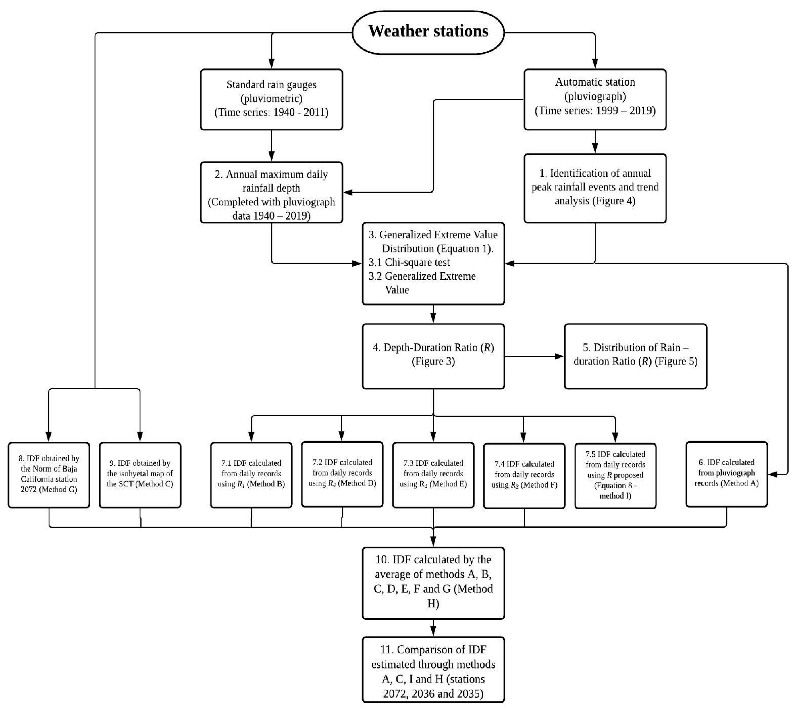
2. Materials and Methods
- IDF calculated from pluviograph records using Gumbel distribution (Equation (1)); this included only three stations (2072, 2036, and 2035).
- IDF calculated from daily records of ten stations (standard rain gauge), using the Chen equation, where (R) was calculated through the weighted average of the from automatic stations, applying Gumbel distribution, implementing (R1).
- IDF obtained by the isohyetal map of the (SCT) only for stations 2072, 2036, 2035, 2001, 2005, and 2045.
- IDF calculated from daily records of ten stations (standard rain gauge), using the Chen equation, where (R) was calculated through the by the modification of Bell equation [28], implementing (R4).
- IDF calculated from daily records of ten stations (standard rain gauge), using the Chen equation, where (R) was calculated through the by the world isopluvial map of Reich [27], implementing (R3).
- IDF obtained by the Norm of the State of Baja California only for station 2072.
- IDF calculated by the average of IDF developed through options A, B, C, D, E, F, and G.
- IDF calculated from daily records of ten stations (standard rain gauge), using Chen equation, where (R) is the ratio proposed calculated by Equation (8).
3. Results and Discussion
4. Conclusions
Supplementary Materials
Author Contributions
Funding
Acknowledgments
Conflicts of Interest
References
- De Paola, F.; Giugni, M.; Topa, M.E.; Bucchignani, E. Intensity-Duration-Frequency (IDF) rainfall curves, for data series and climate projection in African cities. Springer 2014, 3, 1–18. [Google Scholar] [CrossRef] [PubMed]
- Raghunath, H.M. Hydrology Principles-Analysis-Design; New Age International: New Delhi, India, 2006; ISBN 9788122423327. [Google Scholar]
- Sherif, M.; Chowdhury, R.; Shetty, A. Rainfall and Intensity-Duration-Frequency (IDF) Curves in United Arab Emirates. In Proceedings of the World Environmental and Water Resources Congress, Portland, OR, USA, 1–5 June 2014. [Google Scholar]
- Gericke, O.J.; Du Plessis, J.A. Evaluation of the standard design flood method in selected basins in South Africa. J. S. Afr. Inst. Civ. Eng. 2012, 54, 2–14. [Google Scholar]
- Lin, X. Flash Floods in Arid and Semi-Arid Zones; UNESCO: Paris, France, 1999. [Google Scholar]
- Cruz Aguirre, R.U. Además de “Rosa”, Ocho Huracanes más han Pasado a Menos de 200 km de Ensenada. Available online: https://todos.cicese.mx/sitio/noticia.php?n=1215#.XdhI15NKjIV (accessed on 31 August 2020).
- Pacheco, B. Tiene Baja California Historial de Desastres—El Vigía. Available online: https://www.elvigia.net/general/2015/12/10/tiene-baja-california-historial-desastres-220040.html (accessed on 31 August 2020).
- Rodríguez Esteves, J.M. La conformación de los “desastres”—Construcción social del riesgo y variabilidad climática en Tijuana, B.C. Front. Norte 2007, 19, 83–112. [Google Scholar]
- Arnell, V. Analysis of Rainfall Data for Use in Design of Storm Sewer Systems; International Conference on Urban Storm Drainage: Southampton, UK, 1978; pp. 1–15. [Google Scholar]
- Campos-Aranda, D.F. Relación y estimación de predicciones de lluvia horaria-diaria en dos zonas geográficas de México. Tecnol. Cienc. Agua 2012, 3, 141–152. [Google Scholar]
- López-Lambraño, A.; Fuentes, C.; González-Sosa, E.; López-Ramos, A. Pérdidas por intercepción de la vegetación y su efecto en la relación intensidad, duración y frecuencia (IDF) de la lluvia en una cuenca semiárida. Tecnol. Cienc. Agua 2017, 8, 37–56. [Google Scholar]
- DeGaetano, A.T.; Castellano, C.M. Future projections of extreme precipitation intensity-duration-frequency curves for climate adaptation planning in New York State. Clim. Serv. 2017, 5, 23–35. [Google Scholar] [CrossRef]
- Groisman, P.Y.; Knight, R.W.; Karl, T.R. Changes in intense precipitation over the Central United States. J. Hydrometeorol. 2012, 13, 47–66. [Google Scholar] [CrossRef]
- WHO; UNEP. Managing the Risks of Extreme Events and Disasters to Advance Climate Change Adaptation; Cambridge University Press: New York, NY, USA, 2012; p. 594. [Google Scholar]
- Jaklič, A.; Šajn, L.; Derganc, G.; Peer, P. Automatic digitization of pluviograph strip charts. Meteorol. Appl. 2016, 23, 57–64. [Google Scholar] [CrossRef]
- Llasat, M.-C. An Objective Classification of Rainfall Events on the Basis of their Convective Features. Application to Rainfall Intensity in the North-East of Spain. Int. J. Climatol. 2001, 21, 1385–1400. [Google Scholar] [CrossRef]
- Organización Meteorológica Mundial. Guía del Sistema Mundial de Observación; Organización meteorológica mundial: Geneva, Switzerland, 2010; ISBN 9789263304889. [Google Scholar]
- Plummer, N.; Allsopp, T.; Lopez, J.A. Guidelines on Climate Observation Networks and Systems; Llansó, P., Ed.; World Meteorological Organization: Geneva, Switzerland, 2003. [Google Scholar]
- Secretaría de Infraestructura y Desarrollo Urbano. Normas Técnicas para Elaboración de Proyectos de Alcantarillado Pluvial en el Estado de Baja California. 2013. Available online: http://www.ordenjuridico.gob.mx/Documentos/Estatal/Baja%20California/wo83549.pdf (accessed on 31 August 2020).
- Secretaría Comunicaciones y Transporte. Isoyetas de Intensidad-Duración-Periodo de Retorno para la República Mexicana—Baja California; Secretaria Comunicaciones y Transporte: Mexicali, Mexico, 2014; Available online: http://www.sct.gob.mx/carreteras/direccion-general-de-servicios-tecnicos/isoyetas/ (accessed on 31 August 2020).
- SEDATU. Términos de Referencia para Elaborar Atlas de Riesgos; Secretaría de Desarrollo Agrario, Territorial y Urbano: Ciudad de México, Mexico, 2016; p. 121. [Google Scholar]
- Secretaría de Gobernación y Cenapred. Guía Básica para la Elaboración de Atlas Estatales y Municpales de Peligros y Riesgos; Violeta, R., Ed.; Secretaría de Gobernación y Cenapred: Ciudad de México, Mexico, 2014; ISBN 9706289054. [Google Scholar]
- Chen, C. Rainfall intensity-duration-frequency formulas. J. Hydraul. Eng. 1983, 109, 1603–1621. [Google Scholar] [CrossRef]
- Campos-Aranda, D. Intensidades máximas de lluvia para diseño hidrológico urbano en la república mexicana Rainfall Maximum Intensities for Urban Hydrological Design in Mexican Republic. Ing. Investig. Tecnol. 2010, 11, 179–188. [Google Scholar]
- Lorente Castelló, J.; Casas Castillo, M.C.; Rodríguez Sola, R.; Redaño Xipell, Á. Intensidades extremas y precipitación máxima probable. Fenóm. Meteorol. Advers. Esp. 2013, Volumen 5, 142–155. [Google Scholar]
- Hodges, L.H.; Hershfield, D.M.; Washington, D.C.; Reichelderfer, F.W. Rainfall Frequency Atlas of the United States for Durations from 30 Minutes to 24 Hours and Return Periods from 1 to 100 Years; Weather Bureau: Washington, DC, USA, 1961; p. 65. [Google Scholar]
- Reich, B.M. Short-Duration Rainfall-Intensity Estimates and Other Design Aids for Regions of Sparse Data. J. Hydrol. 1963, 1, 3–28. [Google Scholar] [CrossRef]
- Bell, F.C. Generalized Rainfall-Duration-Frequency Relationships. J. Hydraul. Div. 1969, 95, 311–327. [Google Scholar]
- Smith, S.V.; Bullock, S.H.; Hinojosa-Corona, A.; Franco-Vizcaíno, E.; Escoto-Rodríguez, M.; Kretzschmar, T.G.; Farfán, L.M.; Salazar-Ceseña, J.M. Soil erosion and significance for carbon fluxes in a mountainous Mediterranean-climate watershed. Ecol. Appl. 2007, 17, 1379–1387. [Google Scholar] [CrossRef]
- López-Lambraño, A. Elaboración de las Curvas de Intensidad-Duración-Frecuencia de la Lluvia en las Estaciones Pluviográficas Aeropuerto los Garzones, Universidad de Córdoba y Turipana, Localizadas en la Cuenca Media del Río Sinú, Montería; Universidad Pontificia Bolivariana: Montería, CO, USA, 2001. [Google Scholar]
- Maldonado, M.; Martínez, G.; Matajira, F.F. Elaboración curvas IDF estaciones: Cinera Villa Olga y Santa Isabel—Municipio de Cúcuta—Colombia. Rev. Ambient. Agua Aire Suelo 2007, 2, 80–94. [Google Scholar]
- Said, S.E.; Dickey, D.A. Testing for Unit Roots in Autoregressive-Moving Average Models of Unknown Order. Biometrika 1984, 71, 599–607. [Google Scholar] [CrossRef]
- Courty, L.G.; Wilby, R.L.; Hillier, J.K.; Slater, L.J. Intensity-duration-frequency curves at the global scale. Environ. Res. Lett. 2019, 14, 1–11. [Google Scholar] [CrossRef]
- Hersfield, D.M.; Wilson, W.T. Generalizing of Rainfall-Intensity-Frequency Data. AIHS. Gen. Ass. Toronto 1957, 1, 499–506. [Google Scholar]
- López-Lambraño, A.A.; Fuentes, C.; López-Ramos, A.A.; Mata-Ramírez, J.; López-Lambraño, M. Spatial and temporal Hurst exponent variability of rainfall series based on the climatological distribution in a semiarid region in Mexico. Atmosfera 2018, 31, 199–219. [Google Scholar] [CrossRef]
- Poveda, G.; Álvarez, D.M. El colapso de la hipótesis de estacionariedad por cambio y variabilidad climática: Implicaciones para el diseño hidrológico en ingeniería. Rev. Ing. 2012, 36, 65–76. [Google Scholar]
- Frevert, R.; Schwab, G.; Edminster, T.; Barnes, K. Soil and Water Conservation Engineering; John Wiley & Sons Ltd.: New York, NY, USA, 1963. [Google Scholar]
- Robie, R.B. Rainfall Analysis for Drainage Design; Department of Water Resources: Sacramento, CA, USA, 1976. [Google Scholar]
- NOAA’s, N.W.S. NOAA Atlas 14 Point Precipitation Frequency Estimates: CA. Available online: https://hdsc.nws.noaa.gov/hdsc/pfds/pfds_map_cont.html?bkmrk=ca (accessed on 31 August 2020).
- Nhat, M.L.; Tachikawa, Y.; Takara, K. Establishment of Intensity-Duration-Frequency Curves for Precipitation in the Monsoon Area of Vietnam. Annu. Disas. Prev. Res. Inst. 2006, 49B, 93–103. [Google Scholar]
- Tfwala, C.M.; van Rensburg, L.D.; Schall, R.; Mosia, S.M.; Dlamini, P. Precipitation intensity-duration-frequency curves and their uncertainties for Ghaap plateau. Clim. Risk Manag. 2017, 1–9. [Google Scholar] [CrossRef]
- Koutsoyiannis, D.; Kozonis, D.; Manetas, A. A mathematical framework for studying rainfall intensity-duration-frequency relationships. J. Hydrol. 1998, 206, 118–135. [Google Scholar] [CrossRef]
- Sun, Y.; Wendi, D.; Kim, D.E.; Liong, S.Y. Deriving intensity–duration–frequency (IDF) curves using downscaled in situ rainfall assimilated with remote sensing data. Geosci. Lett. 2019, 6, 1–12. [Google Scholar] [CrossRef]
- Domínguez, R.; Carrizosa, E.; Fuentes, G.E.; Arganis, M.L.; Osnaya, J.; Galván-Torres, A.E. Análisis regional para estimar precipitaciones de diseño en la república mexicana. Tecnol. Cienc. Agua 2018, 9, 5–29. [Google Scholar] [CrossRef]


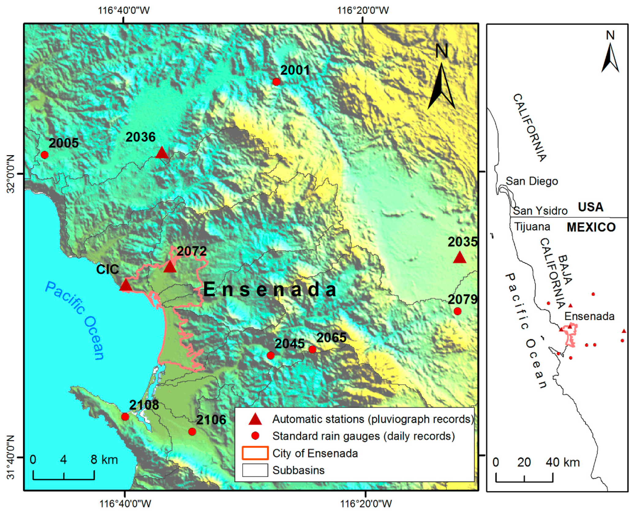
| Station Name | Station ID | Elevation above Sea Level (M) | Type of Records | Lat | Long | Record Length | Source of Data |
|---|---|---|---|---|---|---|---|
| Emilio Lopez Zamora | 2072 | 43 | 10 min 24 h | 31.89 | −116.60 | 1999–2019 1940–2019 | CONAGUA CONAGUA/CICESE |
| CICESE | CIC | 60 | 5 min | 31.86 | −16.66 | 2007–2019 | CICESE |
| Guadalupe | 2036 | 361 | 5 min 24 h | 32.02 | −116.61 | 2009–2019 1954–2019 | CICESE CONAGUA |
| Ojos Negros | 2035 | 680 | 5 min 24 h | 31.91 | −116.23 | 2009–2019 1948–2019 | CICESE CONAGUA |
| Agua Caliente | 2001 | 400 | 24 h | 32.10 | −116.45 | 1969–2011 | CONAGUA |
| Boquilla de Santa Rosa | 2005 | 250 | 24 h | 32.02 | −116.77 | 1969–2011 | CONAGUA |
| San Carlos | 2045 | 164 | 24 h | 31.78 | −116.46 | 1969–2011 | CONAGUA |
| Santo Tomas | 2065 | 180 | 24 h | 31.79 | −116.40 | 1969–2011 | CONAGUA |
| El Alamar | 2079 | 710 | 24 h | 31.83 | −116.20 | 1969–2011 | CONAGUA |
| Maneadero | 2106 | 50 | 24 h | 31.69 | −116.57 | 1969–2011 | CONAGUA |
| Punta Banda | 2108 | 15 | 24 h | 31.71 | −116.66 | 1969–2010 | CONAGUA |
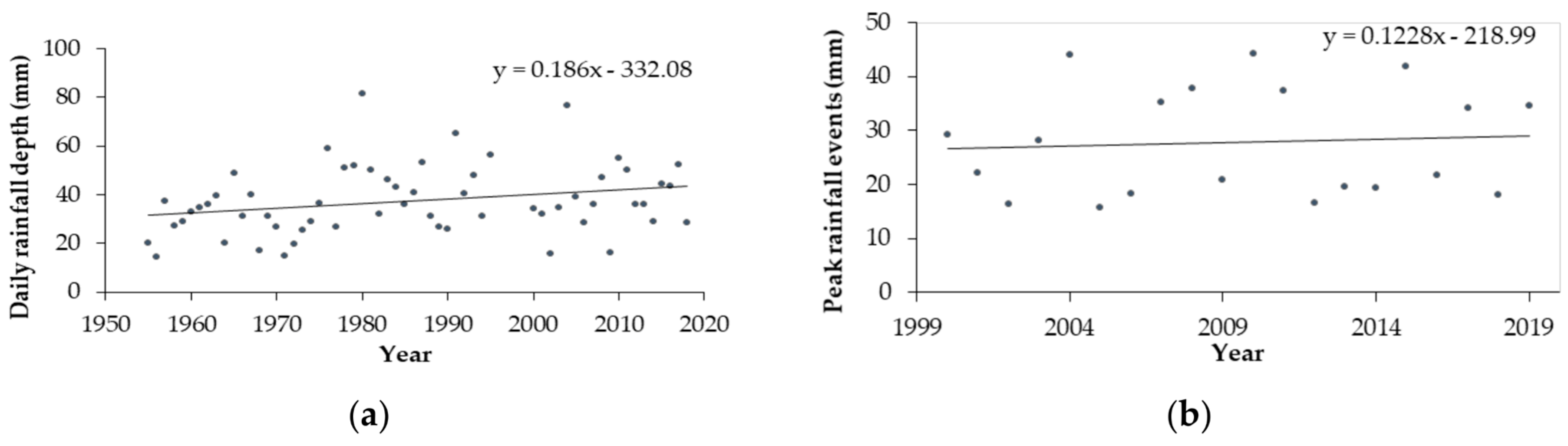
| Peak Rainfall Events (Mm) at Different Durations (ELZ -2072 ) | ||||||
|---|---|---|---|---|---|---|
| Years | 10 min | 20 min | 30 min | 60 min | 120 min | 180 min |
| 1999 | 3.30 | 5.08 | 5.58 | 5.58 | 7.35 | 9.12 |
| 2000 | 6.35 | 8.13 | 8.12 | 10.40 | 14.23 | 20.60 |
| 2001 | 5.59 | 6.85 | 8.12 | 9.14 | 10.90 | 13.40 |
| 2002 | 3.05 | 4.32 | 4.57 | 7.11 | 10.16 | 11.70 |
| 2003 | 2.54 | 3.55 | 5.09 | 6.60 | 11.18 | 12.40 |
| 2004 | 4.83 | 7.11 | 9.14 | 10.90 | 18.79 | 24.60 |
| 2005 | 3.56 | 5.34 | 6.61 | 11.70 | 13.72 | 13.70 |
| 2006 | 4.32 | 7.37 | 9.14 | 12.40 | 18.29 | 18.30 |
| 2007 | 4.32 | 8.13 | 12.19 | 18.03 | 24.37 | 35.30 |
| 2008 | 3.56 | 6.35 | 6.60 | 11.40 | 18.27 | 21.60 |
| 2009 | 4.83 | 6.86 | 9.14 | 11.40 | 17.00 | 18.80 |
| 2010 | 6.86 | 8.89 | 9.65 | 12.20 | 19.56 | 23.40 |
| 2011 | 3.56 | 5.33 | 7.11 | 11.40 | 16.00 | 20.10 |
| 2012 | 4.83 | 5.34 | 6.86 | 9.15 | 16.52 | 16.50 |
| 2013 | 3.05 | 6.10 | 6.61 | 7.61 | 12.95 | 19.60 |
| 2014 | 6.60 | 10.92 | 12.19 | 12.70 | 13.19 | 13.40 |
| 2015 | 6.80 | 9.91 | 12.45 | 13.20 | 21.34 | 22.90 |
| 2016 | 4.32 | 7.62 | 8.38 | 9.90 | 14.21 | 17.80 |
| 2017 | 5.84 | 8.89 | 9.14 | 13.00 | 20.07 | 22.40 |
| 2018 | 3.00 | 4.57 | 6.00 | 7.40 | 9.89 | 13.20 |
| 2019 | 4.40 | 5.60 | 7.40 | 14.60 | 17.40 | 27.60 |
| Data | Alternative Hypothesis (Significance 0.05) | Result | P-Value | |
|---|---|---|---|---|
| 2072 (Rainfall Data) | 10 min | Stationary | Stationary | 0.0382 |
| 20 min | Stationary | Non stationary | 0.2505 | |
| 30 min | Stationary | Non stationary | 0.5175 | |
| 60 min | Stationary | Non stationary | 0.5984 | |
| 120 min | Stationary | Non stationary | 0.7600 | |
| 180 min | Stationary | Non stationary | 0.6485 | |
| 2001 | Stationary | Non stationary | 0.2235 | |
| 2005 | Stationary | Non stationary | 0.2138 | |
| 2035 | Stationary | Non stationary | 0.5035 | |
| 2036 | Stationary | Non stationary | 0.1968 | |
| 2045 | Stationary | Non stationary | 0.0870 | |
| 2065 | Stationary | Non stationary | 0.4364 | |
| 2072 | Stationary | Non stationary | 0.3331 | |
| 2079 | Stationary | Stationary | 0.0380 | |
| 2106 | Stationary | Non stationary | 0.0603 | |
| 2108 | Stationary | Non stationary | 0.0535 | |
| Location of Weather Stations | Rain (mm) | Reference |
|---|---|---|
| Southern California | 12.7 | Frevert et al., 1963 [37] |
| Southern California | 12.7 | Reich, 1963 [27] |
| Ensenada B.C | 14 | Reich, 1963 [27] |
| San Diego | 14.22 | Dedrick et al., 1976 [27] |
| Coronado San Diego, CA | 13.13 Ranges (11.48–16.61) | Hodges et al, 1961 [26] NOAA, 2020 [38] |
| Chula Vista San Diego, CA | 11.63 | NOAA, 2020 [38] |
| Imperial Beach, CA | 10.84 | NOAA, 2020 [38] |
| San Ysidro, CA | Ranges (9.39–13.63) | NOAA, 2020 [38] |
| Northern of Baja California | 10 | CENAPRED, 2016 [22] |
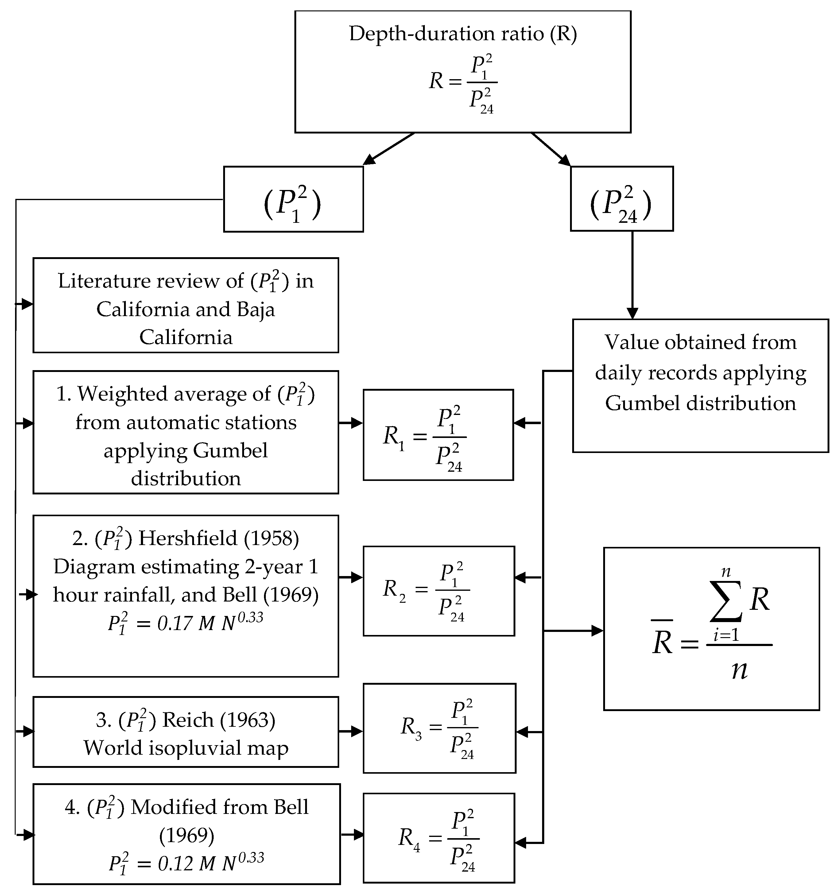
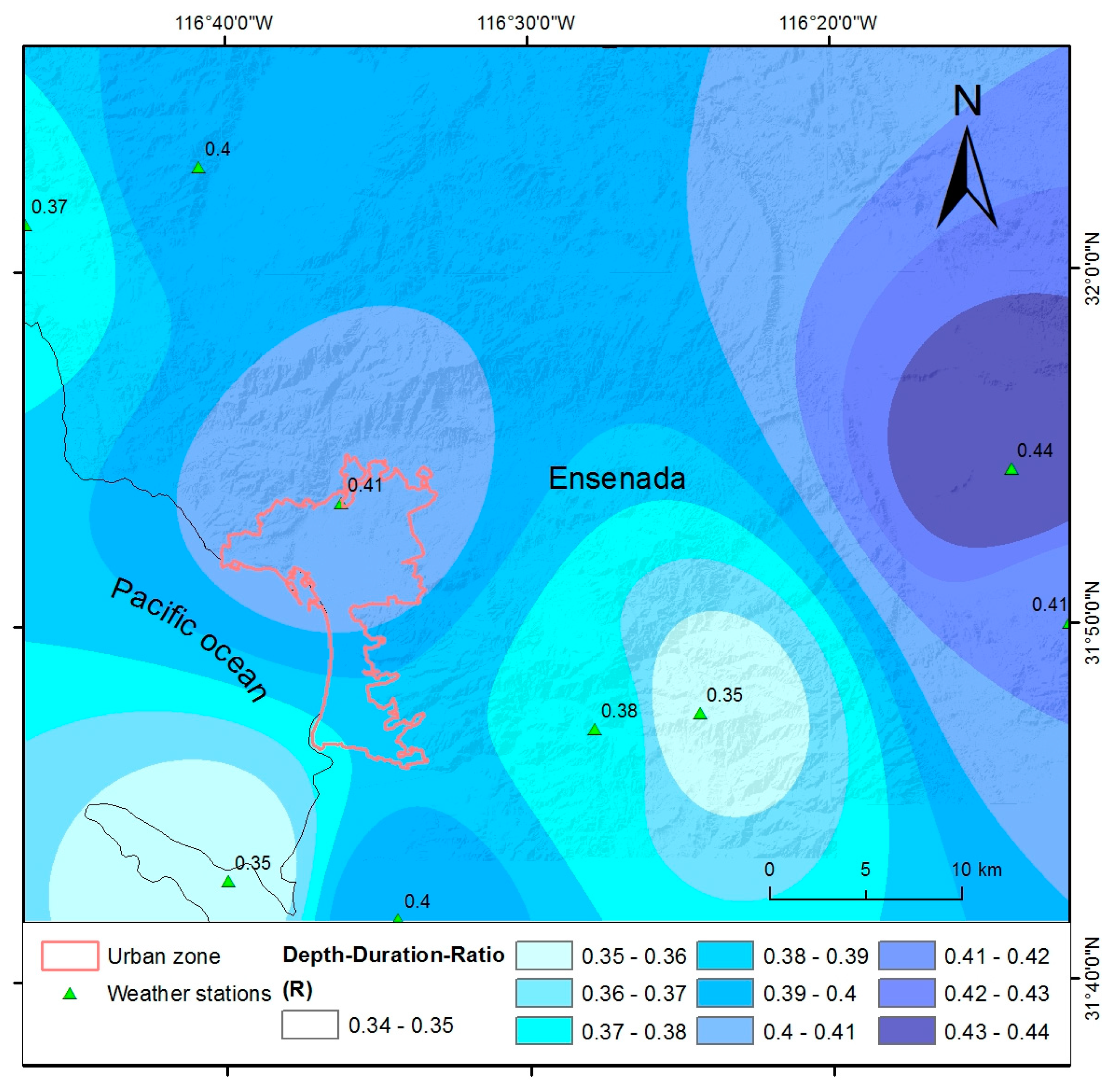
| Station | (mm) | (mm) | (mm) | (mm) | (mm) | R1 | R2 | R3 | R4 | R |
|---|---|---|---|---|---|---|---|---|---|---|
| 2072 | 10.56 | 17.35 | 14.20 | 12.29 | 32.90 | 0.32 | 0.53 | 0.43 | 0.37 | 0.41 |
| 2036 | 11.00 | 21.13 | 13.80 | 14.92 | 38.40 | 0.29 | 0.55 | 0.36 | 0.39 | 0.40 |
| 2035 | 10.96 | 17.13 | 14.50 | 12.09 | 31.20 | 0.35 | 0.55 | 0.47 | 0.39 | 0.44 |
| 2001 | 10.20 | 19.40 | 13.90 | 11.62 | 34.70 | 0.29 | 0.56 | 0.40 | 0.33 | 0.40 |
| 2005 | 10.20 | 23.33 | 13.70 | 12.86 | 41.00 | 0.25 | 0.57 | 0.33 | 0.31 | 0.37 |
| 2045 | 10.20 | 22.38 | 14.50 | 13.02 | 39.90 | 0.26 | 0.56 | 0.36 | 0.33 | 0.38 |
| 2065 | 10.20 | 21.87 | 14.50 | 11.05 | 40.70 | 0.25 | 0.54 | 0.36 | 0.27 | 0.35 |
| 2079 | 10.20 | 20.33 | 14.70 | 12.96 | 35.10 | 0.29 | 0.58 | 0.42 | 0.37 | 0.41 |
| 2106 | 10.20 | 18.34 | 14.50 | 10.80 | 34.00 | 0.30 | 0.54 | 0.43 | 0.32 | 0.40 |
| 2108 | 10.20 | 21.22 | 14.5 | 10.16 | 39.70 | 0.26 | 0.53 | 0.36 | 0.26 | 0.35 |
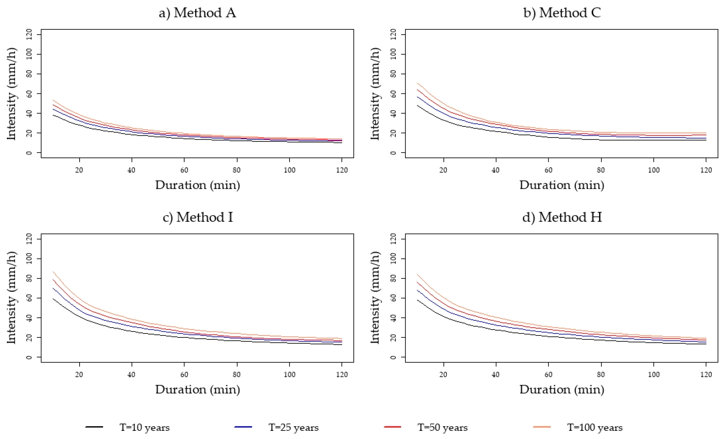
| Return Period | IDF (mm/hr) Station 2072 | |||||
|---|---|---|---|---|---|---|
| Method | 10 (min) | 20 (min) | 30 (min) | 60 (min) | 120 (min) | |
| 10 years | (A) | 38.3 | 28.1 | 22.3 | 14.6 | 10.5 |
| (B) | 45.2 | 32.2 | 25.8 | 17.2 | 11.2 | |
| (C) | 48.0 | 38.0 | 26.0 | 16.0 | 13.0 | |
| (D) | 52.8 | 37.8 | 30.1 | 19.7 | 12.5 | |
| (E) | 59.6 | 42.7 | 33.9 | 21.8 | 13.5 | |
| (F) | 70.6 | 50.8 | 40.1 | 25.1 | 14.9 | |
| (G) | 99.2 | 59.0 | 43.5 | 25.9 | 15.4 | |
| Average | 59.1 | 41.2 | 31.7 | 20.0 | 13.0 | |
| 25 years | (A) | 44.3 | 32.4 | 25.6 | 16.7 | 12.0 |
| (B) | 53.3 | 38.0 | 30.5 | 20.3 | 13.2 | |
| (C) | 57.0 | 40.0 | 31.0 | 20.0 | 15.0 | |
| (D) | 62.4 | 44.6 | 35.5 | 23.2 | 14.7 | |
| (E) | 70.3 | 50.4 | 40.1 | 25.7 | 15.9 | |
| (F) | 83.4 | 60.0 | 47.3 | 29.7 | 17.6 | |
| (G) | 119.0 | 70.0 | 52.0 | 31.0 | 18.0 | |
| Average | 70.0 | 47.9 | 37.4 | 23.8 | 15.2 | |
| 50 years | (A) | 48.7 | 35.5 | 28.0 | 18.2 | 13.1 |
| (B) | 59.5 | 42.5 | 34.0 | 22.6 | 14.7 | |
| (C) | 64.0 | 45.0 | 35.0 | 22.0 | 18.0 | |
| (D) | 69.6 | 49.7 | 39.6 | 25.9 | 16.4 | |
| (E) | 78.5 | 56.3 | 44.7 | 28.7 | 17.7 | |
| (F) | 93.0 | 66.9 | 52.8 | 33.1 | 19.7 | |
| (G) | 134.7 | 80.1 | 59.1 | 35.1 | 20.9 | |
| Average | 78.3 | 53.7 | 41.9 | 25.8 | 17.0 | |
| 100 years | (A) | 53.1 | 38.7 | 30.4 | 19.7 | 14.2 |
| (B) | 65.7 | 46.9 | 37.5 | 25.0 | 16.3 | |
| (C) | 71.0 | 50.0 | 38.0 | 24.0 | 20.0 | |
| (D) | 76.8 | 54.9 | 43.8 | 28.6 | 18.1 | |
| (E) | 86.6 | 62.1 | 49.3 | 31.7 | 19.6 | |
| (F) | 102.7 | 73.9 | 58.3 | 36.6 | 21.7 | |
| (G) | 150.0 | 89.2 | 65.8 | 39.1 | 23.3 | |
| Average | 86.6 | 59.4 | 46.2 | 29.2 | 19.0 | |
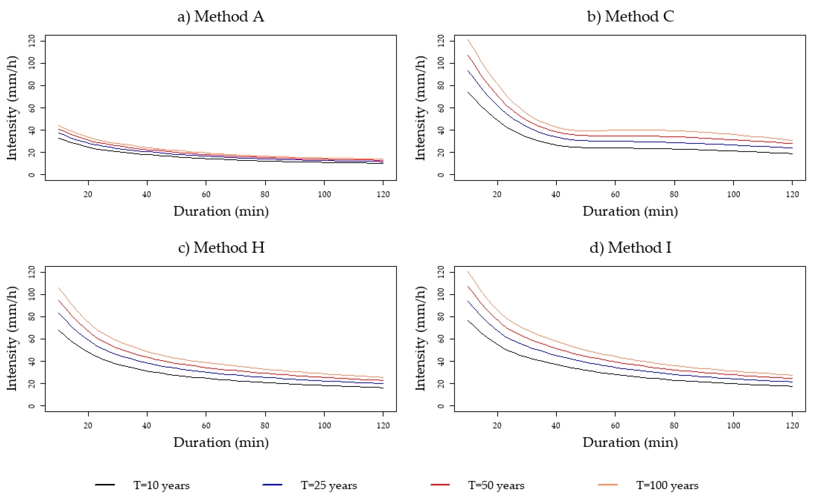
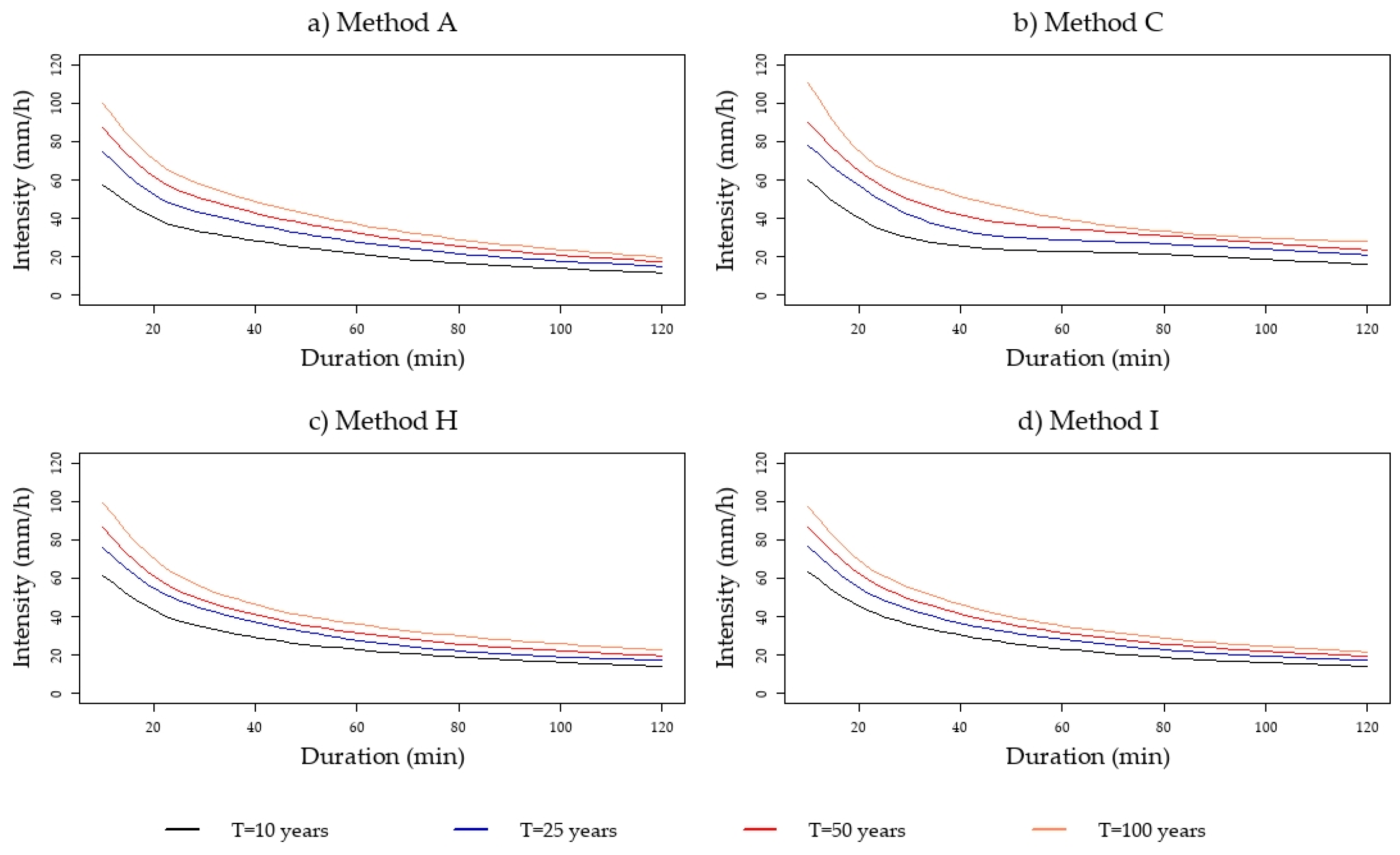
| Return Period | Stations | Intensity Duration Frequency (mm/h) for Different Durations | ||||
|---|---|---|---|---|---|---|
| 10 (min) | 20 (min) | 30 (min) | 60 (min) | 120 (min) | ||
| 10 years | 2072 | 57.71 | 41.35 | 32.86 | 21.22 | 13.21 |
| 2036 | 76.70 | 54.92 | 43.68 | 28.30 | 17.69 | |
| 2035 | 63.58 | 45.63 | 36.19 | 23.17 | 14.22 | |
| 2001 | 68.68 | 49.18 | 39.11 | 25.34 | 15.84 | |
| 2005 | 76.61 | 54.76 | 43.66 | 28.55 | 18.12 | |
| 2045 | 66.59 | 47.62 | 37.93 | 24.73 | 15.61 | |
| 2065 | 68.58 | 48.97 | 39.11 | 25.76 | 16.51 | |
| 2079 | 71.32 | 51.10 | 40.61 | 26.23 | 16.32 | |
| 2106 | 61.60 | 44.11 | 35.08 | 22.73 | 14.21 | |
| 2108 | 74.84 | 53.44 | 42.68 | 28.11 | 18.02 | |
| 25 years | 2072 | 68.15 | 48.83 | 38.80 | 25.06 | 15.59 |
| 2036 | 93.96 | 67.28 | 53.51 | 34.66 | 21.67 | |
| 2035 | 76.82 | 55.14 | 43.73 | 28.00 | 17.18 | |
| 2001 | 83.95 | 60.12 | 47.81 | 30.97 | 19.36 | |
| 2005 | 94.00 | 67.19 | 53.56 | 35.03 | 22.23 | |
| 2045 | 79.00 | 56.51 | 45.01 | 29.34 | 18.53 | |
| 2065 | 83.28 | 59.47 | 47.50 | 31.28 | 20.05 | |
| 2079 | 87.28 | 62.54 | 49.70 | 32.10 | 19.97 | |
| 2106 | 73.74 | 52.81 | 41.99 | 27.21 | 17.01 | |
| 2108 | 93.09 | 66.48 | 53.09 | 34.97 | 22.42 | |
| 50 years | 2072 | 76.04 | 54.48 | 43.30 | 27.96 | 17.40 |
| 2036 | 107.01 | 76.63 | 60.94 | 39.48 | 24.68 | |
| 2035 | 86.85 | 62.33 | 49.43 | 31.65 | 19.43 | |
| 2001 | 95.50 | 68.39 | 54.38 | 35.23 | 22.03 | |
| 2005 | 107.15 | 76.59 | 61.06 | 39.94 | 25.34 | |
| 2045 | 88.39 | 63.22 | 50.36 | 32.83 | 20.73 | |
| 2065 | 94.41 | 67.41 | 53.84 | 35.46 | 22.73 | |
| 2079 | 99.36 | 71.19 | 56.57 | 36.54 | 22.74 | |
| 2106 | 82.92 | 59.38 | 47.22 | 30.59 | 19.13 | |
| 2108 | 106.90 | 76.34 | 60.97 | 40.15 | 25.74 | |
| 100 years | 2072 | 83.93 | 60.14 | 47.79 | 30.87 | 19.21 |
| 2036 | 120.07 | 85.98 | 68.38 | 44.30 | 27.70 | |
| 2035 | 96.87 | 69.52 | 55.13 | 35.30 | 21.67 | |
| 2001 | 107.05 | 76.66 | 60.96 | 39.49 | 24.69 | |
| 2005 | 120.30 | 85.99 | 68.55 | 44.84 | 28.45 | |
| 2045 | 97.79 | 69.94 | 55.71 | 36.32 | 22.93 | |
| 2065 | 105.53 | 75.35 | 60.18 | 39.63 | 25.41 | |
| 2079 | 111.43 | 79.84 | 63.45 | 40.98 | 25.50 | |
| 2106 | 92.11 | 65.96 | 52.45 | 33.98 | 21.25 | |
| 2108 | 120.71 | 86.20 | 68.84 | 45.34 | 29.07 | |
Publisher’s Note: MDPI stays neutral with regard to jurisdictional claims in published maps and institutional affiliations. |
© 2020 by the authors. Licensee MDPI, Basel, Switzerland. This article is an open access article distributed under the terms and conditions of the Creative Commons Attribution (CC BY) license (http://creativecommons.org/licenses/by/4.0/).
Share and Cite
Gámez-Balmaceda, E.; López-Ramos, A.; Martínez-Acosta, L.; Medrano-Barboza, J.P.; Remolina López, J.F.; Seingier, G.; Daesslé, L.W.; López-Lambraño, A.A. Rainfall Intensity-Duration-Frequency Relationship. Case Study: Depth-Duration Ratio in a Semi-Arid Zone in Mexico. Hydrology 2020, 7, 78. https://doi.org/10.3390/hydrology7040078
Gámez-Balmaceda E, López-Ramos A, Martínez-Acosta L, Medrano-Barboza JP, Remolina López JF, Seingier G, Daesslé LW, López-Lambraño AA. Rainfall Intensity-Duration-Frequency Relationship. Case Study: Depth-Duration Ratio in a Semi-Arid Zone in Mexico. Hydrology. 2020; 7(4):78. https://doi.org/10.3390/hydrology7040078
Chicago/Turabian StyleGámez-Balmaceda, Ena, Alvaro López-Ramos, Luisa Martínez-Acosta, Juan Pablo Medrano-Barboza, John Freddy Remolina López, Georges Seingier, Luis Walter Daesslé, and Alvaro Alberto López-Lambraño. 2020. "Rainfall Intensity-Duration-Frequency Relationship. Case Study: Depth-Duration Ratio in a Semi-Arid Zone in Mexico" Hydrology 7, no. 4: 78. https://doi.org/10.3390/hydrology7040078
APA StyleGámez-Balmaceda, E., López-Ramos, A., Martínez-Acosta, L., Medrano-Barboza, J. P., Remolina López, J. F., Seingier, G., Daesslé, L. W., & López-Lambraño, A. A. (2020). Rainfall Intensity-Duration-Frequency Relationship. Case Study: Depth-Duration Ratio in a Semi-Arid Zone in Mexico. Hydrology, 7(4), 78. https://doi.org/10.3390/hydrology7040078