Use of Teleconnections to Predict Western Australian Seasonal Rainfall Using ARIMAX Model


Abstract
1. Introduction
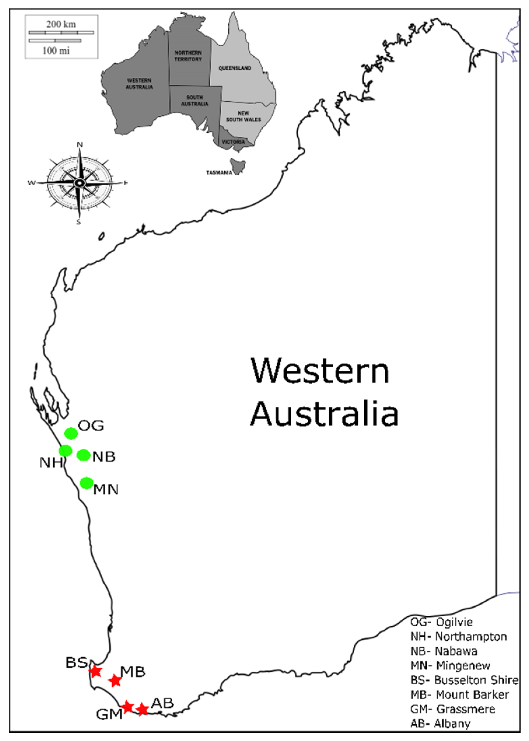
2. Data and Study Area
3. Methodology
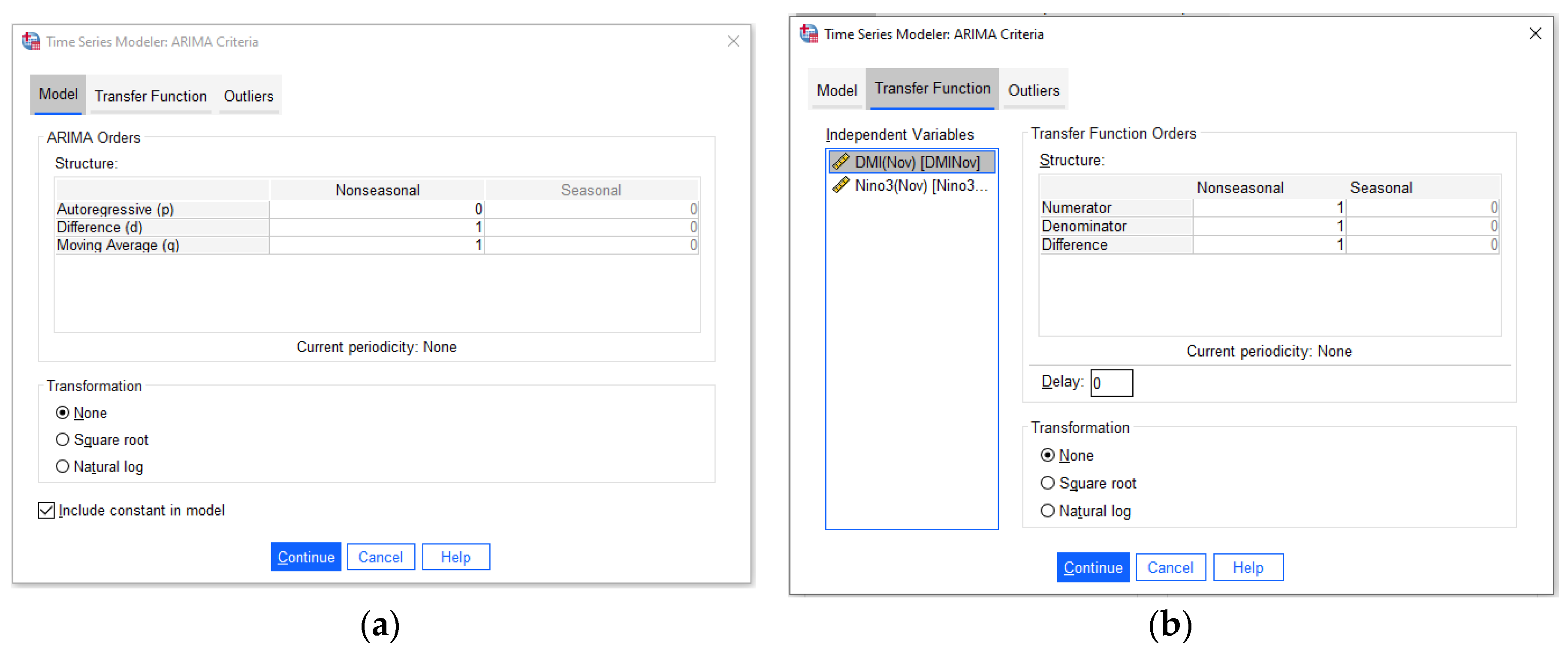
3.1. Multivariate Auto–Regressive Integrated Moving Average with Exogenous Input (ARIMAX)
- Autoregressive (p): it is defined as the number of autoregressive orders in the model. Autoregressive orders specify which previous values from the series are used to predict the present values.
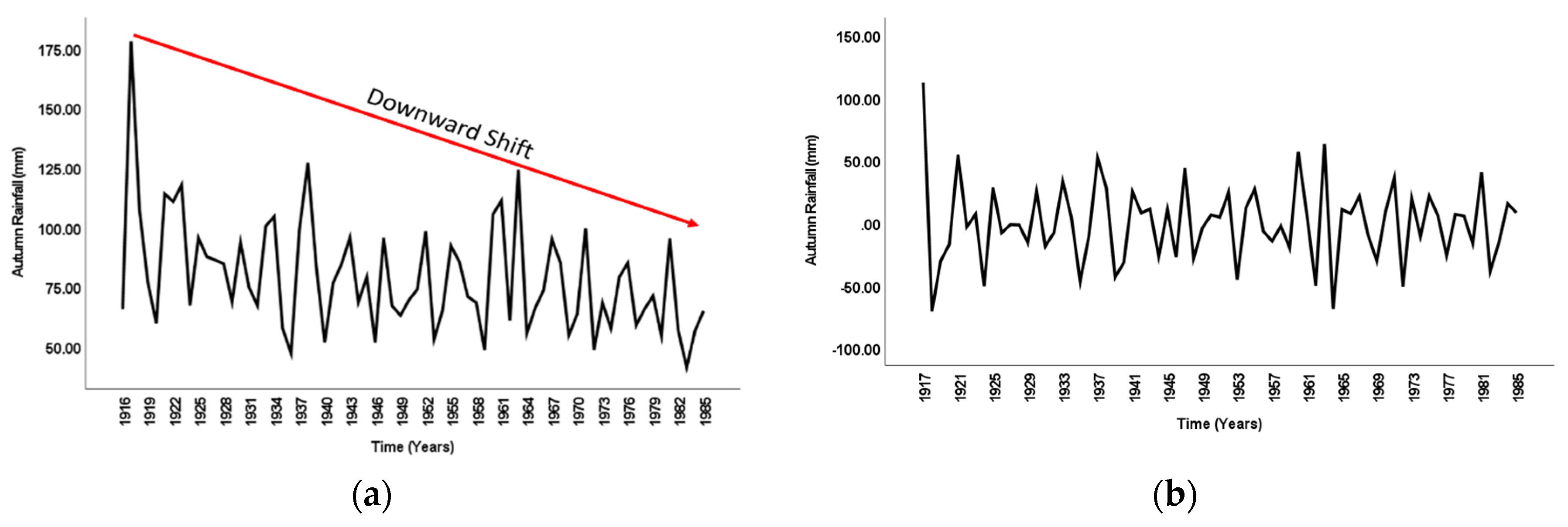
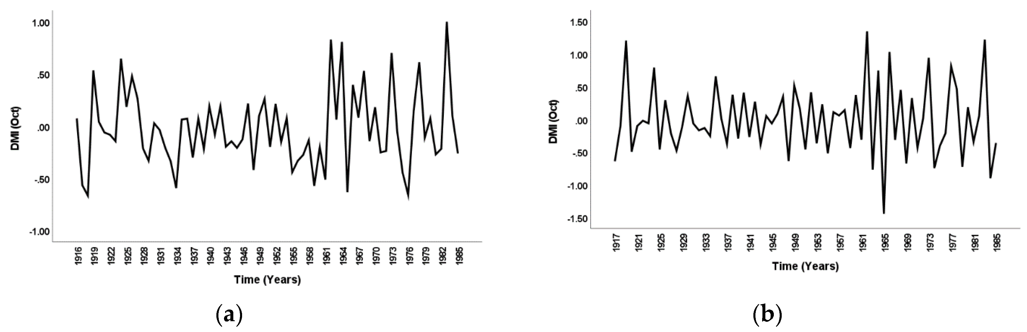
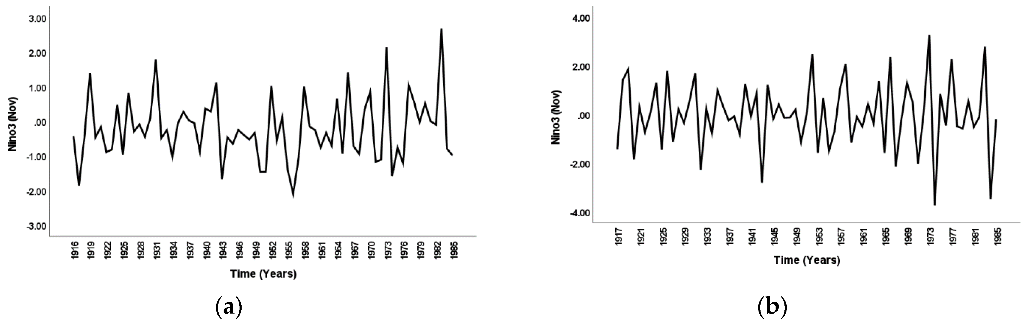
- Difference (d):it is defined as the order of differencing in the model. Differencing is necessary to make a non–stationary series into stationary series. As the ARIMA model is stationary, it is necessary to remove the non–stationary effects before estimating models. A first–order differencing is often proved as enough for linear trends, while a second–order differencing is required for quadratic trend.
- Moving Average (q): it is defined as the number of moving average orders in the model. Moving average orders specify how deviation from the series mean of previous values (past errors) is used to predict current values. Therefore, it is the number of lagged forecast errors in the predicted equation.
- Numerator: it is the number of orders of the numerator in the transfer function. It states which past values of independent series are used to predict the current value of the dependent series. Such as a numerator value of 1 states that the one–time period past value and the current value of an independent series are used to predict the current values of the dependent series.
- Denominator: it is the number of orders of the denominator in the transfer function. It is specified to predict the current value of the dependent series and how deviations from the series mean for previous values of independent variables are used. For instance, a denominator number of 1 indicates that the deviation from the mean of the independent series one period in the past is considered to predict the current values of the dependent series.
- Difference: it is the order of differencing. It is applied to make a non–stationary series into stationary before estimating the model.
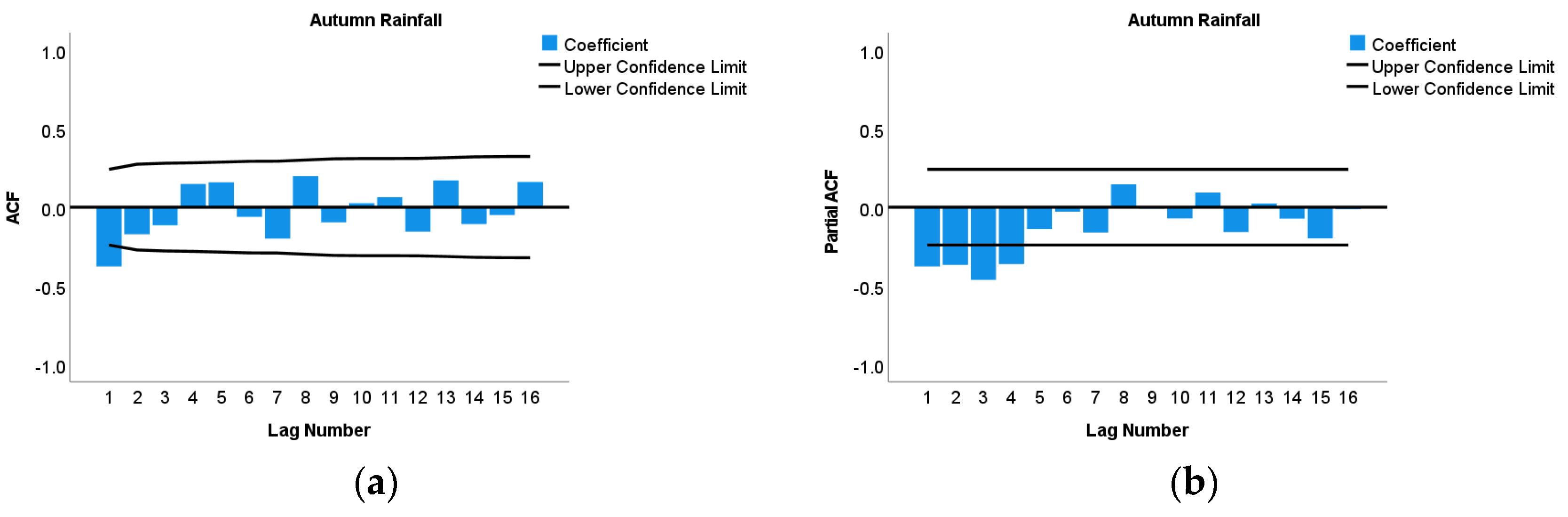
- Identification: in this stage, first, the raw data series is plotted to identify whether the data is stationary or not. If the raw data series is found to be non–stationary, differencing is required. After the first order differencing, correlograms of the autocorrelation function (ACF) and partial autocorrelation function (PACF) is investigated. From these plots, the order of AR and MA gets identified.
- Parameter Estimation and Selection: the number of AR depends on the lag of PACF cuts and the number of MA depends on the lag of the ACF plot. However, decision making on the order of AR and MA by looking at the cuts/spikes is not straightforward. Most of the time it required experimentation with several alternative orders of different models to choose the appropriate order. The following guidelines are usually followed during the selection of the AR and MA order:
- If the ACF plot shows exponential decay and PACF spikes at lag–1, no correlation for other lags, in that case, one autoregressive parameter (p = 1) can be selected.
- If the ACF plot shows a sine–wave shape pattern or a set of exponential decay and PACF spikes at lag–1 and lag–2, no correlation for other lags, in that case, two autoregressive parameters (p = 2) can be selected.
- If the PACF plot shows exponential decay and ACF spikes at lag–1, no correlation for other lags, in that case, one moving average parameter (q = 1) can be selected.
- If the PACF plot shows a sine–wave shape pattern or a set of exponential decay and ACF spikes at lag–1 and lag–2, no correlation for other lags, in that case, two moving average parameters (q = 2) can be selected.
- One auto–regressive and one moving average parameter can be selected if both shows exponential decay starting at lag–1.
- Sometimes, using both AR and MA orders in a model can cancel each other’s impact. Therefore, it is often wise to use mixed AR and MA models with less number of orders.
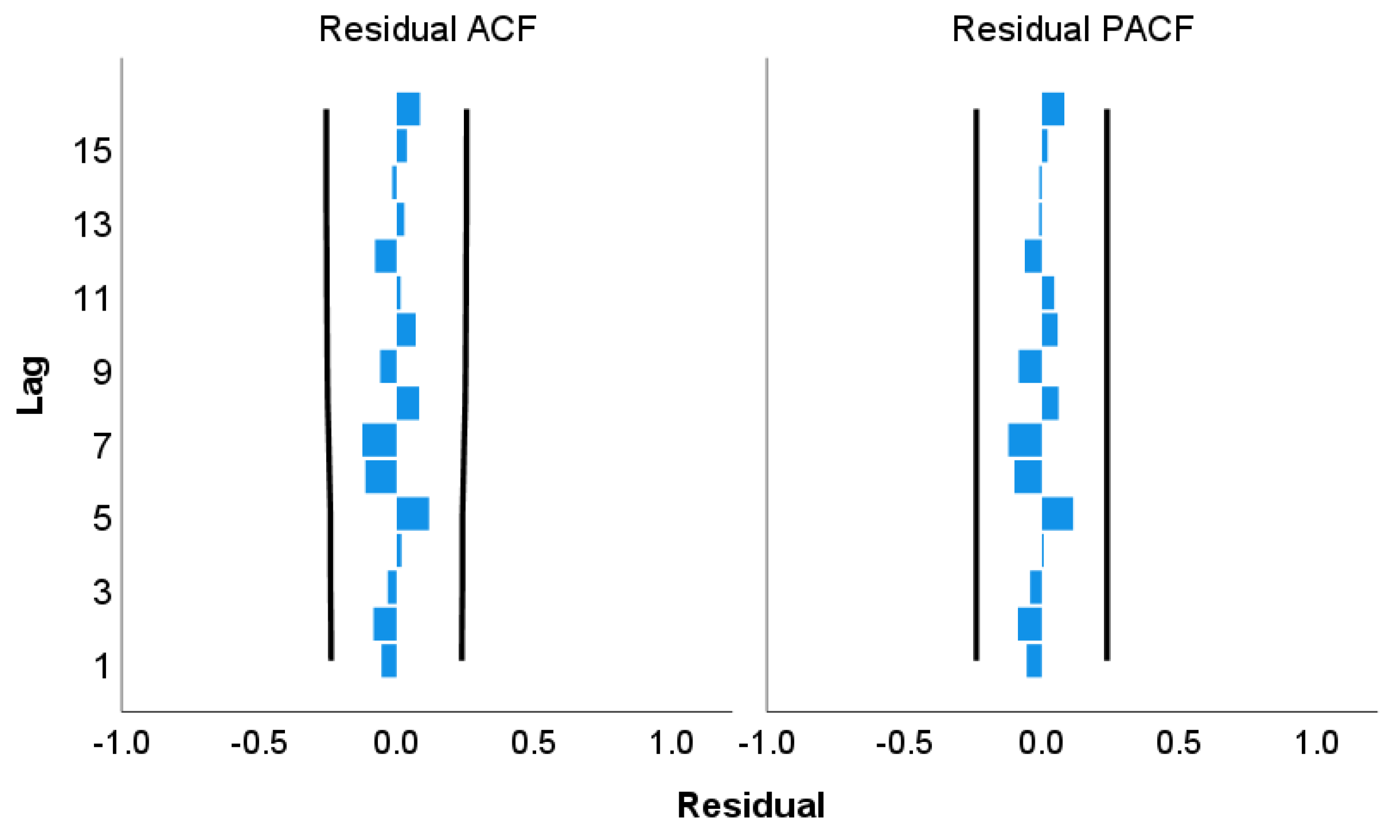
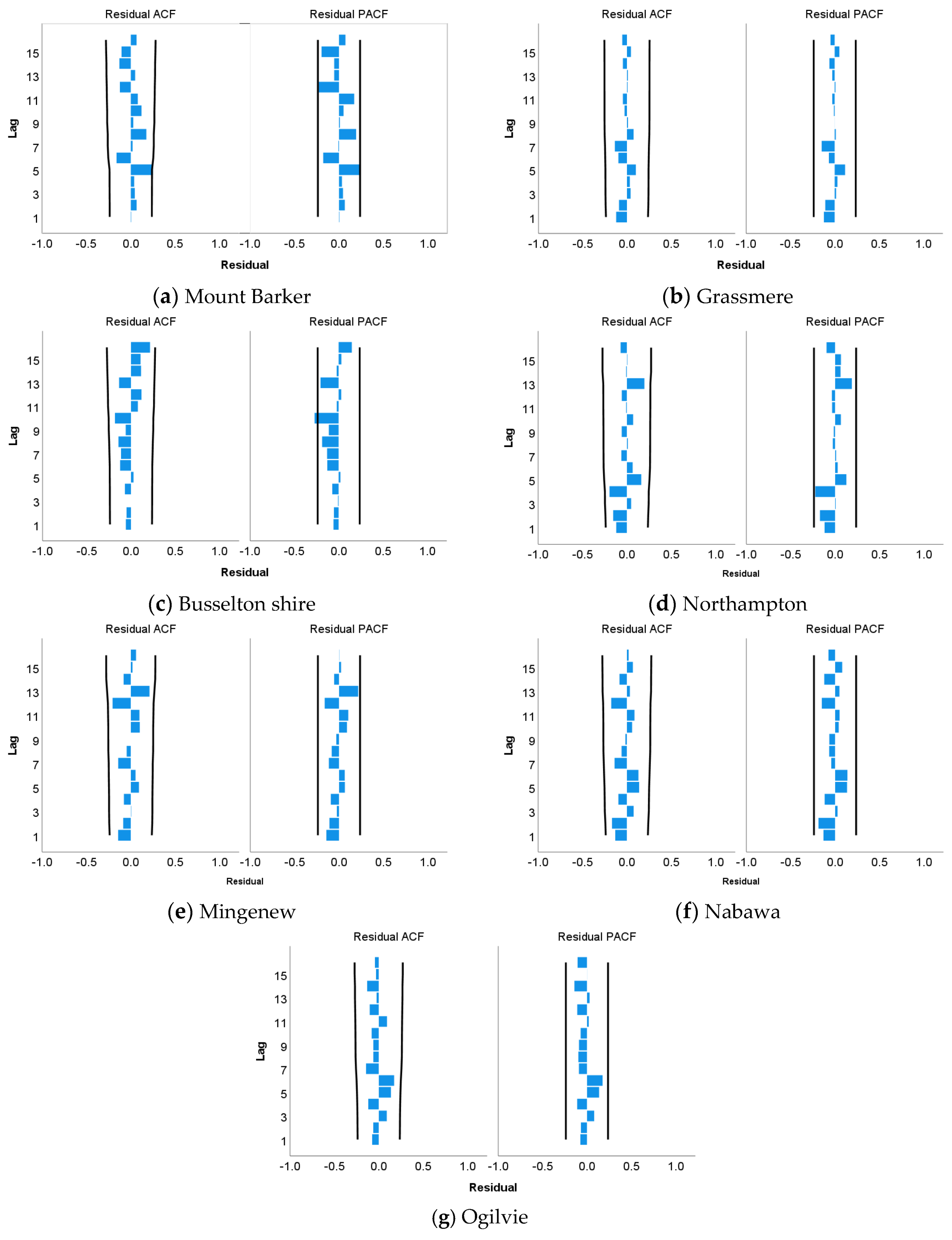
- Diagnostics Check: the diagnostic check is required to verify the adequacy of the developed model. The residual of the developed model should be white noise (no autocorrelation). To check whether the residual is white noise or not, at first, an inspection of the residual ACF and PACF plot is required. If 95% of the spikes stay between the black lines, it indicates that the autocorrelation is white noise. If two or more spikes or more than 5% of spikes are located outside of the boundary line, then the series is not white noise. Another way of checking the model accuracy is to perform the Ljung–Box test. Such a test is conducted to verify the null hypothesis of being white noise of residual if the p–value is greater than 0.05 [68]. A p–value greater than 0.05 implies that lag autocorrelation among the residuals is zero and the developed model is adequate to fit the data set.
3.2. Statistical Parameters for ARIMAX Model
4. Results
5. Discussion
6. Conclusions
Author Contributions
Funding
Acknowledgments
Conflicts of Interest
Appendix A


Appendix B


References
- Goddard, L.; Mason, S.J.; Zebiak, S.E.; Ropelewski, C.F.; Basher, R.; Cane, M.A. Current approaches to seasonal to interannual climate predictions. Int. J. Climatol. 2001, 21, 1111–1152. [Google Scholar] [CrossRef]
- Anderson, J.; van den Dool, H.; Barnston, A.; Chen, W. Present-day capabilities of numerical and statistical models for atmospheric extratropical seasonal simulation and prediction. Bull. Am. Meteorol. Soc. 1999, 80, 1349–1362. [Google Scholar] [CrossRef]
- Schepen, A.; Wang, Q.; Robertson, D. Evidence for using lagged climate indices to forecast Australian seasonal rainfall. J. Clim. 2012, 25, 1230–1246. [Google Scholar] [CrossRef]
- Li, J.; Wang, B. Origins of the decadal predictability of East Asian land summer monsoon rainfall. J. Clim. 2018, 31, 6229–6243. [Google Scholar] [CrossRef]
- Li, J.; Wang, B.; Yang, Y.M. Retrospective seasonal prediction of summer monsoon rainfall over West Central and Peninsular India in the past 142 years. Clim. Dyn. 2017, 48, 2581–2596. [Google Scholar] [CrossRef]
- Momani, P.; Naill, P. Time series analysis model for rainfall data in Jordan: Case study for using time series analysis. Am. J. Environ. Sci. 2009, 5, 599. [Google Scholar] [CrossRef]
- Mondal, P.; Shit, L.; Goswami, S. Study of effectiveness of time series modeling (ARIMA) in forecasting stock prices. Int. J. Comput. Sci. Eng. Appl. 2014, 4, 13. [Google Scholar] [CrossRef]
- Tularam, G. Relationship between El Niño southern oscillation index and rainfall (Queensland, Australia). Int. J. Sustain. Dev. Plan. 2010, 5, 378–391. [Google Scholar] [CrossRef]
- Brown, K.; Kamruzzaman, M.; Beecham, S. Trends in sub-daily precipitation in Tasmania using regional dynamically downscaled climate projections. J. Hydrol. Reg. Stud. 2017, 10, 18–34. [Google Scholar] [CrossRef]
- Kamruzzaman, M.; Beecham, S.; Metcalfe, A. Climatic influences on rainfall and runoff variability in the southeast region of the Murray-Darling Basin. Int. J. Climatol. 2013, 33, 291–311. [Google Scholar] [CrossRef]
- Kamruzzaman, M.; Beecham, S.; Metcalfe, A. Estimation of trends in rainfall extremes with mixed effects models. Atmos. Res. 2016, 168, 24–32. [Google Scholar] [CrossRef]
- Kamruzzaman, M.; Beecham, S.; Metcalfe, A.V.; Cai, W. Granger causal predictors for maximum rainfall in Australia. Atmos. Res. 2019, 218, 1–11. [Google Scholar] [CrossRef]
- Bloomfield, P. Trends in global temperature. Clim. Chang. 1992, 21, 1–16. [Google Scholar] [CrossRef]
- Cohn, T.A.; Lins, H.F. Nature’s style: Naturally trendy. Geophys. Res. Lett. 2005, 32, L23402. [Google Scholar] [CrossRef]
- Kamruzzaman, M.; Metcalfe, A.V.; Beecham, S. Wavelet-based rainfall–stream flow models for the southeast Murray darling basin. J. Hydrol. Eng. 2013, 19, 1283–1293. [Google Scholar] [CrossRef]
- Kumar, K.K.; Soman, M.; Kumar, K.R. Seasonal forecasting of Indian summer monsoon rainfall: A review. Weather 1995, 50, 449–467. [Google Scholar] [CrossRef]
- Otok, B.W.; Suhartono, F. Development of rainfall forecasting model in Indonesia by using ASTAR, transfer function, and ARIMA methods. Eur. J. Sci. Res. 2009, 38, 386–395. [Google Scholar]
- Weeks, W.; Boughton, W. Tests of ARMA model forms for rainfall-runoff modelling. J. Hydrol. 1987, 91, 29–47. [Google Scholar] [CrossRef]
- Han, P.; Wang, P.X.; Zhang, S.Y.; Zhu, D.H. Drought forecasting based on the remote sensing data using ARIMA models. Math. Comput. Model. 2010, 51, 1398–1403. [Google Scholar] [CrossRef]
- Zhang, G.P. Time series forecasting using a hybrid ARIMA and neural network model. Neurocomputing 2003, 50, 159–175. [Google Scholar] [CrossRef]
- Cai, W.; van Rensch, P.; Cowan, T.; Hendon, H.H. Teleconnection pathways of ENSO and the IOD and the mechanisms for impacts on Australian rainfall. J. Clim. 2011, 24, 3910–3923. [Google Scholar] [CrossRef]
- Drosdowsky, W.; Williams, M. The Southern Oscillation in the Australian region. Part I: Anomalies at the extremes of the oscillation. J. Clim. 1991, 4, 619–638. [Google Scholar] [CrossRef]
- Kirono, D.G.; Chiew, F.H.; Kent, D.M. Identification of best predictors for forecasting seasonal rainfall and runoff in Australia. Hydrol. Process. 2010, 24, 1237–1247. [Google Scholar] [CrossRef]
- McBride, J.L.; Nicholls, N. Seasonal relationships between Australian rainfall and the Southern Oscillation. Mon. Weather Rev. 1983, 111, 1998–2004. [Google Scholar] [CrossRef]
- Islam, F.; Imteaz, M.A. Development of prediction model for forecasting rainfall in Western Australia using lagged climate indices. Int. J. Water 2019, 13, 248–268. [Google Scholar] [CrossRef]
- Risbey, J.S.; Pook, M.J.; McIntosh, P.C.; Wheeler, M.C.; Hendon, H.H. On the remote drivers of rainfall variability in Australia. Mon. Weather Rev. 2009, 137, 3233–3253. [Google Scholar] [CrossRef]
- Chiew, F.H.; Piechota, T.C.; Dracup, J.A.; McMahon, T.A. El Nino/Southern Oscillation and Australian rainfall, streamflow and drought: Links and potential for forecasting. J. Hydrol. 1998, 204, 138–149. [Google Scholar] [CrossRef]
- Chowdhury, R.K.; Beecham, S. Influence of SOI, DMI and Niño3. 4 on South Australian rainfall. Stoch. Environ. Res. Risk Assess. 2013, 27, 1909–1920. [Google Scholar] [CrossRef]
- Drosdowsky, W.; Chambers, L.E. Near-global sea surface temperature anomalies as predictors of Australian seasonal rainfall. J. Clim. 2001, 14, 1677–1687. [Google Scholar] [CrossRef]
- Feng, J.; Li, J.; Li, Y. Is there a relationship between the SAM and southwest Western Australian winter rainfall? J. Clim. 2010, 23, 6082–6089. [Google Scholar] [CrossRef]
- Fierro, A.O.; Leslie, L.M. Links between central west Western Australian rainfall variability and large-scale climate drivers. J. Clim. 2013, 26, 2222–2246. [Google Scholar] [CrossRef]
- Marshall, A.; Hendon, H. Impacts of the MJO in the Indian Ocean and on the Western Australian coast. Clim. Dyn. 2014, 42, 579–595. [Google Scholar] [CrossRef]
- Montazerolghaem, M.; Vervoort, W.; Minasny, B.; McBratney, A. Long-term variability of the leading seasonal modes of rainfall in south-eastern Australia. Weather Clim. Extrem. 2016, 13, 1–14. [Google Scholar] [CrossRef]
- Ramsay, H.A.; Leslie, L.M.; Lamb, P.J.; Richman, M.B.; Leplastrier, M. Interannual variability of tropical cyclones in the Australian region: Role of large-scale environment. J. Clim. 2008, 21, 1083–1103. [Google Scholar] [CrossRef]
- Rasel, H.; Imteaz, M.; Mekanik, F. Investigating the influence of Remote Climate Drivers as the Predictors in Forecasting South Australian spring rainfall. Int. J. Environ. Res. 2016, 10, 1–12. [Google Scholar]
- Ummenhofer, C.C.; Gupta, A.S.; Pook, M.J.; England, M.H. Anomalous rainfall over southwest Western Australia forced by Indian Ocean sea surface temperatures. J. Clim. 2008, 21, 5113–5134. [Google Scholar] [CrossRef]
- Zhu, Z. Breakdown of the relationship between Australian summer rainfall and ENSO caused by tropical Indian Ocean SST warming. J. Clim. 2018, 31, 2321–2336. [Google Scholar] [CrossRef]
- Cai, W.; van Rensch, P.; Cowan, T.; Hendon, H.H. An asymmetry in the IOD and ENSO teleconnection pathway and its impact on Australian climate. J. Clim. 2012, 25, 6318–6329. [Google Scholar] [CrossRef]
- Ashok, K.; Guan, Z.; Yamagata, T. Influence of the Indian Ocean Dipole on the Australian winter rainfall. Geophys. Res. Lett. 2003, 30, 1821. [Google Scholar] [CrossRef]
- Saji, N.; Goswami, B.; Vinayachandran, P.; Yamagata, T. A dipole mode in the tropical Indian Ocean. Nature 1999, 401, 360. [Google Scholar] [CrossRef]
- Smith, I. Indian ocean sea-surface temperature patterns and australian winter rainfall. Int. J. Climatol. 1994, 14, 287–305. [Google Scholar] [CrossRef]
- Ashok, K.; Guan, Z.; Yamagata, T. A Look at the Relationship between the ENSO and the Indian Ocean Dipole. J. Meteorol. Soc. Jpn. 2003, 81, 41–56. [Google Scholar] [CrossRef]
- Forootan, E.; Awange, J.; Schumacher, M.; Anyah, R.; van Dijk, A.; Kusche, J. Quantifying the impacts of ENSO and IOD on rain gauge and remotely sensed precipitation products over Australia. Remote Sens. Environ. 2016, 172, 50–66. [Google Scholar] [CrossRef]
- Hasan, M.; Dunn, P.K. Understanding the effect of climatology on monthly rainfall amounts in Australia using Tweedie GLMs. Int. J. Climatol. 2012, 32, 1006–1017. [Google Scholar] [CrossRef]
- Islam, F.; Imteaz, M.A.; Boulomytis, V.G.; Rasel, H. Combined regression modelling of autumn rainfall in Western Australia using potential climate indices. In 37th Hydrology & Water Resources Symposium 2016: Water, Infrastructure and the Environment; Engineers Australia: Barton, Australia, 2016. [Google Scholar]
- Mekanik, F.; Imteaz, M.; Gato-Trinidad, S.; Elmahdi, A. Multiple regression and Artificial Neural Network for long-term rainfall forecasting using large scale climate modes. J. Hydrol. 2013, 503, 11–21. [Google Scholar] [CrossRef]
- Abbot, J.; Marohasy, J. Application of artificial neural networks to rainfall forecasting in Queensland, Australia. Adv. Atmos. Sci. 2012, 29, 717–730. [Google Scholar] [CrossRef]
- Choubin, B.; Khalighi-Sigaroodi, S.; Malekian, A.; Ahmad, S.; Attarod, P. Drought forecasting in a semi-arid watershed using climate signals: A neuro-fuzzy modeling approach. J. Mt. Sci. 2014, 11, 1593–1605. [Google Scholar] [CrossRef]
- Choubin, B.; Khalighi-Sigaroodi, S.; Malekian, A.; Kişi, Ö. Multiple linear regression, multi-layer perceptron network and adaptive neuro-fuzzy inference system for forecasting precipitation based on large-scale climate signals. Hydrol. Sci. J. 2016, 61, 1001–1009. [Google Scholar] [CrossRef]
- Choubin, B.; Malekian, A.; Golshan, M. Application of several data-driven techniques to predict a standardized precipitation index. Atmósfera 2016, 29, 121–128. [Google Scholar] [CrossRef]
- Choubin, B.; Malekian, A.; Samadi, S.; Khalighi-Sigaroodi, S.; Sajedi-Hosseini, F. An ensemble forecast of semi-arid rainfall using large-scale climate predictors. Meteorol. Appl. 2017, 24, 376–386. [Google Scholar] [CrossRef]
- Choubin, B.; Zehtabian, G.; Azareh, A.; Rafiei-Sardooi, E.; Sajedi-Hosseini, F.; Kişi, Ö. Precipitation forecasting using classification and regression trees (CART) model: A comparative study of different approaches. Environ. Earth Sci. 2018, 77, 314. [Google Scholar] [CrossRef]
- Kisi, O.; Choubin, B.; Deo, R.C.; Yaseen, Z.M. Incorporating synoptic-scale climate signals for streamflow modelling over the Mediterranean region using machine learning models. Hydrol. Sci. J. 2019, 64, 1240–1252. [Google Scholar] [CrossRef]
- Chadsuthi, S.; Modchang, C.; Lenbury, Y.; Iamsirithaworn, S.; Triampo, W. Modeling seasonal leptospirosis transmission and its association with rainfall and temperature in Thailand using time–series and ARIMAX analyses. Asian Pac. J. Trop. Med. 2012, 5, 539–546. [Google Scholar] [CrossRef]
- Fan, J.; Shan, R.; Cao, X.; Li, P. The analysis to tertiary-industry with ARIMAX model. J. Math. Res. 2009, 1, 156. [Google Scholar] [CrossRef]
- Ling, A.; Darmesah, G.; Chong, K.; Ho, C. Application of ARIMAX Model to Forecast Weekly Cocoa Black Pod Disease Incidence. Math. Stat. 2019, 7, 29–40. [Google Scholar]
- Peter, Ď.; Silvia, P. ARIMA vs. ARIMAX–which approach is better to analyze and forecast macroeconomic time series. In Proceedings of the 30th International Conference Mathematical Methods in Economics, Karviná, Czech Republic, 11–13 September 2012. [Google Scholar]
- Jalalkamali, A.; Moradi, M.; Moradi, N. Application of several artificial intelligence models and ARIMAX model for forecasting drought using the Standardized Precipitation Index. Int. J. Environ. Sci. Technol. 2015, 12, 1201–1210. [Google Scholar] [CrossRef]
- Taschetto, A.S.; England, M.H. El Niño Modoki impacts on Australian rainfall. J. Clim. 2009, 22, 3167–3174. [Google Scholar] [CrossRef]
- Ashok, K.; Behera, S.K.; Rao, S.A.; Weng, H.; Yamagata, T. El Niño Modoki and its possible teleconnection. J. Geophys. Res. Ocean. 2007, 112, C11007. [Google Scholar] [CrossRef]
- Hossain, I.; Rasel, H.; Imteaz, M.A.; Mekanik, F. Long-term seasonal rainfall forecasting: Efficiency of linear modelling technique. Environ. Earth Sci. 2018, 77, 280. [Google Scholar] [CrossRef]
- Mahmud, I.; Bari, S.H.; Rahman, M.; Mahmud, I.; Bari, S.H.; Rahman, M.T.U. Monthly rainfall forecast of Bangladesh using autoregressive integrated moving average method. Environ. Eng. Res. 2016, 22, 162–168. [Google Scholar] [CrossRef]
- Mehdizadeh, S.; Sales, A.K. A comparative study of autoregressive, autoregressive moving average, gene expression programming and Bayesian networks for estimating monthly streamflow. Water Resour. Manag. 2018, 32, 3001–3022. [Google Scholar] [CrossRef]
- IBM SPSS Forecasting 22; IBM Corporation: Armonk, NY, USA, 2013.
- Box, G.E.; Jenkins, G.M. Time Series Analysis: Forecasting and Control; Revised Ed.; Holden-Day: San Francisco, CA, USA, 1976. [Google Scholar]
- Hamilton, J. Time Series Analysis Princeton University Press Princeton; Princeton University Press: Princeton, NJ, USA, 1994. [Google Scholar]
- Cryer, J.D.; Chan, K.-S. Time Series Analysis: With Applications in R; Springer Science & Business Media: Berlin, Germany, 2008. [Google Scholar]
- Ljung, G.M.; Box, G.E. On a measure of lack of fit in time series models. Biometrika 1978, 65, 297–303. [Google Scholar] [CrossRef]
- Saigal, S.; Mehrotra, D. Performance comparison of time series data using predictive data mining techniques. Adv. Inf. Min. 2012, 4, 57–66. [Google Scholar]
- Singh, J.; Knapp, H.V.; Arnold, J.; Demissie, M. Hydrological modeling of the Iroquois river watershed using HSPF and SWAT 1. J. Am. Water Resour. Assoc. 2005, 41, 343–360. [Google Scholar] [CrossRef]
- Willmott, C.J.; Robeson, S.M.; Matsuura, K. A refined index of model performance. Int. J. Climatol. 2012, 32, 2088–2094. [Google Scholar] [CrossRef]
- Wang, Q.; Schepen, A.; Robertson, D.E. Merging seasonal rainfall forecasts from multiple statistical models through Bayesian model averaging. J. Clim. 2012, 25, 5524–5537. [Google Scholar] [CrossRef]
- Ghamariadyan, M.; Imteaz, M.; Mekanik, F. A hybrid wavelet neural network (HWNN) for forecasting rainfall using temperature and climate indices. IOP Conf. Ser. Earth Environ. Sci. 2019, 351, 012003. [Google Scholar] [CrossRef]
- Field, A. Discovering Statistics Using IBM SPSS Statistics; Sage: London, UK, 2013. [Google Scholar]


| Region | Station Number | Station Name | Latitude | Longitude | Elevation (m) | Annual Mean Rainfall (mm) | Summer Rainfall (mm) | Autumn Rainfall (mm) | Winter Rainfall (mm) | Spring Rainfall (mm) |
|---|---|---|---|---|---|---|---|---|---|---|
| South Coast | 9500 | Albany | 35.03° S | 117.88° E | 3 | 938.2 | 80.7 | 225.0 | 399.4 | 228.7 |
| 9581 | Mount Barker | 34.63° S | 117.64° E | 300 | 733.3 | 80.7 | 157.6 | 283.5 | 189.0 | |
| 9551 | Grassmere | 35.02° S | 117.76° E | 10 | 987.8 | 85.8 | 236.8 | 421.7 | 238.5 | |
| 9515 | Busselton Shire | 33.66° S | 115.35° E | 4 | 811.6 | 32.7 | 177.2 | 446.5 | 149.2 | |
| North Coast | 8104 | Ogilvie | 28.15° S | 114.67° E | 280 | 387.7 | 26.7 | 99.6 | 206.9 | 53.3 |
| 8028 | Nabawa | 28.50° S | 114.79° E | 145 | 450.6 | 25.6 | 104.8 | 251.0 | 67.1 | |
| 8088 | Mingenew | 29.19° S | 115.44° E | 153 | 402.1 | 28.4 | 97.9 | 211.3 | 61.4 | |
| 8100 | Northampton | 28.35° S | 114.64° E | 180 | 450.6 | 22.8 | 122.7 | 269.2 | 68.4 |
| Climate Indices | Region | |||||||
|---|---|---|---|---|---|---|---|---|
| South Coast Rainfall Stations | North Coast Rainfall Stations | |||||||
| Pearson Correlation (r) | Pearson Correlation (r) | |||||||
| Albany | Mount Barker | Grassmere | Busselton Shire | Northampton | Mingenew | Nabawa | Ogilvie | |
| DMIOct | −0.309 ** | −0.242 * | −0.274 * | −0.266 * | −−−− | −−−− | −−−− | −−−− |
| DMINov | −0.375 ** | −−−− | −0.325 ** | −−−− | −−−− | 0.240 * | −−−− | −−−− |
| DMIDec | −0.266 * | −−−− | −−−− | −0.243 * | −−−− | −−−− | −−−− | −−−− |
| DMIJan | −−−− | −−−− | −−−− | −−−− | 0.251 * | −−−− | −−−− | −−−− |
| DMIFeb | −−−− | −−−− | −−−− | −−−− | 0.375 ** | −−−− | 0.287 * | 0.267 * |
| SOIOct | −−−− | −−−− | −−−− | −−−− | −−−− | −−−− | −−−− | −−−− |
| SOINov | 0.254 * | −−−− | −−−− | −−−− | −−−− | 0.242 * | −−−− | −−−− |
| SOIDec | 0.401 ** | −−−− | 0.329 ** | −−−− | −−−− | −−−− | −−−− | −−−− |
| SOIJan | 0.269 * | −−−− | −−−− | −−−− | 0.252 * | 0.256 * | 0.249 * | 0.275 * |
| SOIFeb | 0.346 ** | 0.299 * | 0.301 * | −−−− | −−−− | −−−− | 0.238 * | 0.236 * |
| Nino3.4Oct | −−−− | −−−− | −−−− | −−−− | −−−− | −0.254 * | −0.265 * | −0.243 * |
| Nino3.4Nov | −0.267 * | −0.254 * | −−−− | −0.253 * | −0.255 * | −0.265 * | −0.281 * | −0.259 * |
| Nino3.4Dec | −0.251 * | −−−− | −−−− | −−−− | −0.281 * | −0.290 * | −0.307 ** | −0.291 * |
| Nino3.4Jan | −0.352 ** | −0.302 * | −0.271 * | −0.284 * | −−−− | −0.262 * | −0.251 * | −−−− |
| Nino3.4Feb | −0.382 ** | −0.366 ** | −0.316 ** | −0.282 * | −0.298 * | −0.320 ** | −0.297 * | −0.286 * |
| Nino3Oct | −0.253 * | −0.243 * | −−−− | −0.247 * | −0.256 * | −0.244 * | −0.258 * | −0.249 * |
| Nino3Nov | −0.329 ** | −0.317 ** | −0.271 * | −0.288 * | −0.273 * | −0.273 * | −0.285 * | −0.280 * |
| Nino3Dec | −0.301 * | −0.264 * | −−−− | −−−− | −0.255 * | −0.255 * | −0.264 * | −0.259 * |
| Nino3 Jan | −0.348 ** | −0.291 * | −0.260 * | −0.272 * | −−−− | −−−− | −−−− | −−−− |
| Nino3Feb | −0.365 ** | −0.360 ** | −0.300 * | −0.244 * | −−−− | −0.245 * | −−−− | −−−− |
| Nino4Oct | −−−− | −−−− | −−−− | −−−− | −0.245 * | −0.240 * | −−−− | |
| Nino4Nov | −−−− | −−−− | −−−− | −−−− | −0.254 * | −0.258 * | −−−− | |
| Nino4Dec | −−−− | −−−− | −−−− | −−−− | −0.280 * | −0.313 ** | −0.322 ** | −0.292 * |
| Nino4Jan | −0.332 ** | −0.282 * | −0.280 * | −0.275 * | −0.287 * | −0.344 ** | −0.318 ** | −0.296 * |
| Nino4Feb | −0.327 ** | −0.299 * | −0.272 * | −0.255 * | −0.330 ** | −0.366 ** | −0.334 ** | −0.308 ** |
| EMIOct | −−−− | −−−− | −−−− | −−−− | −−−− | −−−− | −−−− | −−−− |
| EMINov | −−−− | −−−− | −−−− | −−−− | −−−− | −−−− | −−−− | −−−− |
| EMIDec | −−−− | −−−− | −−−− | −−−− | −−−− | −0.269 * | −0.265 * | −−−− |
| EMIJan | −−−− | −−−− | −−−− | −−−− | −0.236 * | −0.330 ** | −0.301 * | −0.251 * |
| EMIFeb | −−−− | −−−− | −−−− | −−−− | −−−− | −0.262 * | −0.259 * | −−−− |
| Region | Station Name | Autoregressive | Difference | Moving Average |
|---|---|---|---|---|
| South Coast | Albany | 0 | 1 | 1 |
| Mount Barker | 2 | 1 | 1 | |
| Grass mere | 0 | 1 | 1 | |
| Busselton Shire | 4 | 1 | 1 | |
| North Coast | Northampton | 0 | 1 | 1 |
| Mingenew | 0 | 1 | 1 | |
| Nabawa | 0 | 1 | 1 | |
| Ogilvie | 0 | 1 | 1 |
| Region | Station Name | Predictors | Numerator | Denominator | Difference |
|---|---|---|---|---|---|
| South Coast | Albany | DMIOct | 1 | 1 | 1 |
| Nino3Nov | |||||
| Mount Barker | DMIOct | 1 | 1 | 1 | |
| Nino3Nov | |||||
| Grass mere | DMIOct | 1 | 1 | 1 | |
| Nino3Nov | |||||
| Busselton Shire | DMIOct | 1 | 1 | 1 | |
| Nino3Nov | |||||
| North Coast | Northampton | DMIJan | 1 | 1 | 1 |
| Nino3Nov | |||||
| Mingenew | DMINov | 1 | 1 | 1 | |
| Nino3Nov | |||||
| Nabawa | DMIFeb | 1 | 1 | 1 | |
| Nino3Nov | |||||
| Ogilvie | DMIFeb | 1 | 1 | 1 | |
| Nino3Nov |
| Region | Station Name | Pearson Correlation (r) for Different Model Sets | ||||
|---|---|---|---|---|---|---|
| DMI–Nino3 | DMI–Nino4 | DMI–Nino3.4 | DMI–SOI | DMI–EMI | ||
| South Coast | Albany | 0.60 | 0.55 | 0.57 | 0.62 | −−− |
| Mount Barker | 0.67 | 0.59 | 0.57 | 0.55 | −−− | |
| Grassmere | 0.64 | 0.64 | 0.60 | 0.57 | −−− | |
| Busselton Shire | 0.58 | 0.56 | 0.56 | −−− | −−− | |
| North Coast | Northampton | 0.82 | 0.81 | 0.81 | 0.75 | 0.78 |
| Mingenew | 0.56 | 0.55 | 0.54 | 0.56 | 0.54 | |
| Nabawa | 0.69 | 0.66 | 0.68 | 0.57 | 0.61 | |
| Ogilvie | 0.66 | 0.61 | 0.64 | 0.58 | 0.53 | |
| Region | Rainfall Station | Model Type | Lag Month | Model Fit Statistics | Ljung–Box Q (18) | ||||||
|---|---|---|---|---|---|---|---|---|---|---|---|
| r | RMSE | MAPE | MAE | Normalized BIC | Statistics | DF | Sig (p) | ||||
| South Coast | Albany 1 | ARIMAX (0,1,1) | 4 | 0.60 | 18.57 | 19.01 | 13.93 | 6.60 | 23.04 | 17 | 0.15 |
| Mount Barker 1 | ARIMAX (2,1,1) | 4 | 0.67 | 16.92 | 22.19 | 12.13 | 6.34 | 14.39 | 15 | 0.49 | |
| Grassmere 1 | ARIMAX (0,1,1) | 4 | 0.64 | 18.85 | 19.84 | 14.48 | 6.69 | 11.76 | 17 | 0.81 | |
| Busselton Shire 1 | ARIMAX (4,1,1) | 4 | 0.58 | 21.58 | 29.31 | 15.56 | 6.95 | 14.14 | 13 | 0.36 | |
| North Coast | Northampton 2 | ARIMAX (0,1,1) | 2 | 0.82 | 13.59 | 27.56 | 9.79 | 5.96 | 29.25 | 17 | 0.13 |
| Mingenew 3 | ARIMAX (0,1,1) | 4 | 0.56 | 15.55 | 38.03 | 11.53 | 6.04 | 16.34 | 17 | 0.50 | |
| Nabawa 4 | ARIMAX (0,1,1) | 1 | 0.69 | 14.19 | 30.56 | 10.26 | 5.93 | 20.06 | 17 | 0.27 | |
| Ogilvie 4 | ARIMAX (0,1,1) | 1 | 0.66 | 16.17 | 32.37 | 11.66 | 6.13 | 13.71 | 17 | 0.68 | |
| Region | Station Name | Model Type | Predictors | Lag Month | Pearson’s Correlation (r) | Refined Willmot Index of Agreement ( ) | ||
|---|---|---|---|---|---|---|---|---|
| Calibration | Validation | Calibration | Validation | |||||
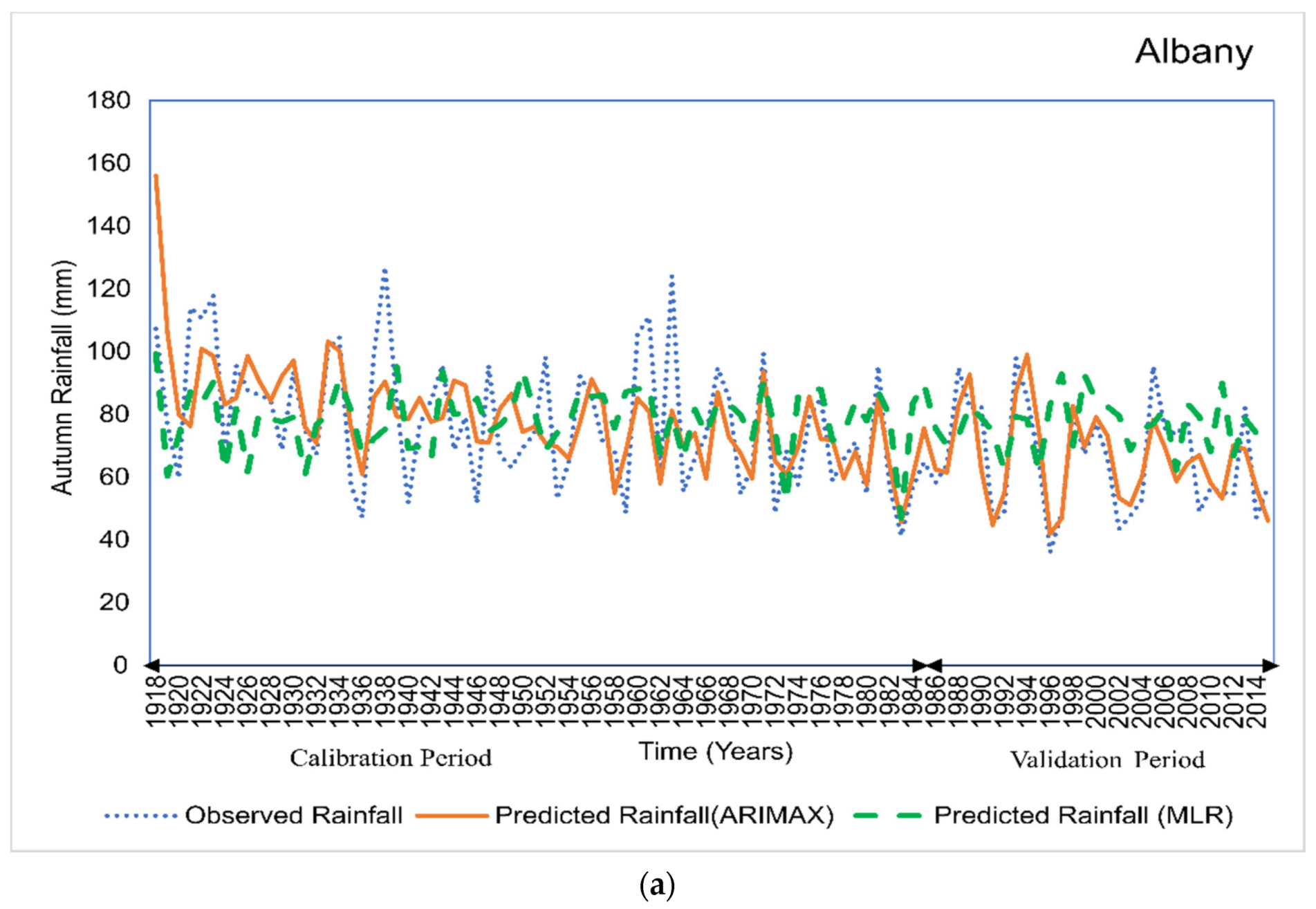
| South Coast | Albany | ARIMAX | DMIOct–Nino3Nov | 4 | 0.60 | 0.80 | 0.61 | 0.71 |
| MLR | DMINov–Nino3Feb | 1 | 0.44 | 0.49 | 0.54 | 0.55 | ||
| Mount Barker | ARIMAX | DMIOct–Nino3Nov | 4 | 0.67 | 0.66 | 0.61 | 0.60 | |
| MLR | DMIOct–Nino3Feb | 1 | 0.37 | 0.42 | 0.54 | 0.51 | ||
| Grassmere | ARIMAX | DMIOct–Nino3Nov | 4 | 0.64 | 0.72 | 0.61 | 0.64 | |
| MLR | DMINov–Nino3Feb | 1 | 0.37 | 0.39 | 0.51 | 0.52 | ||
| Busselton Shire | ARIMAX | DMIOct–Nino3Nov | 4 | 0.58 | 0.62 | 0.61 | 0.61 | |
| MLR | DMIDec–Nino3Nov | 3 | 0.34 | 0.29 | 0.50 | 0.40 | ||
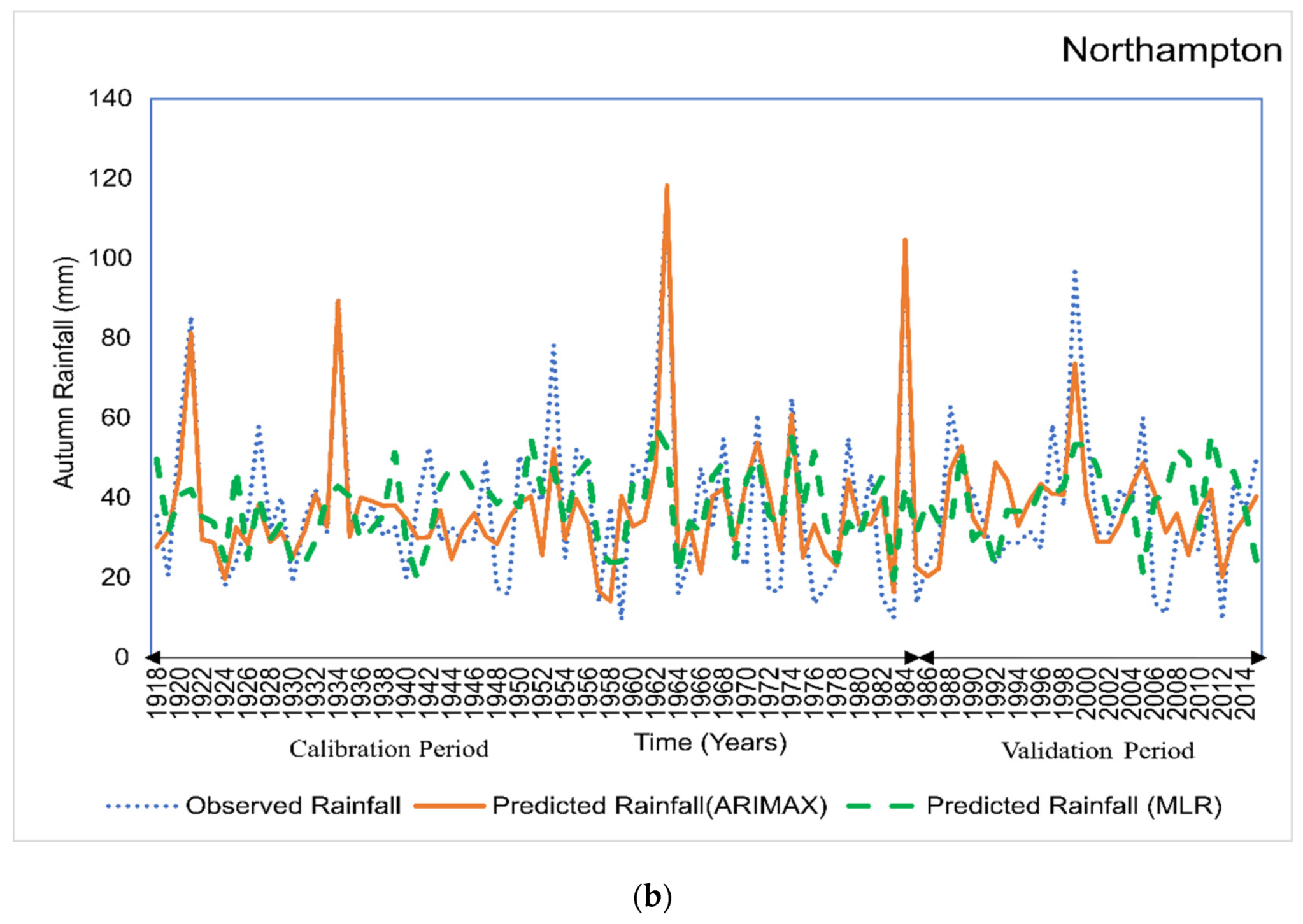
| North Coast | Northampton | ARIMAX | DMIJan–Nino3Nov | 2 | 0.82 | 0.70 | 0.70 | 0.61 |
| MLR | DMIFeb–Nino4Feb | 1 | 0.44 | 0.48 | 0.55 | 0.56 | ||
| Mingenew | ARIMAX | DMINov–Nino3Nov | 4 | 0.56 | 0.62 | 0.56 | 0.50 | |
| MLR | DMINov–Nino4Feb | 1 | 0.38 | 0.44 | 0.52 | 0.55 | ||
| Nabawa | ARIMAX | DMIFeb–Nino3Nov | 1 | 0.69 | 0.66 | 0.63 | 0.56 | |
| MLR | DMIFeb–Nino4Feb | 1 | 0.39 | 0.43 | 0.53 | 0.54 | ||
| Ogilvie | ARIMAX | DMIFeb–Nino3Nov | 1 | 0.66 | 0.68 | 0.61 | 0.64 | |
| MLR | DMIFeb–Nino4Feb | 1 | 0.36 | 0.42 | 0.52 | 0.53 | ||
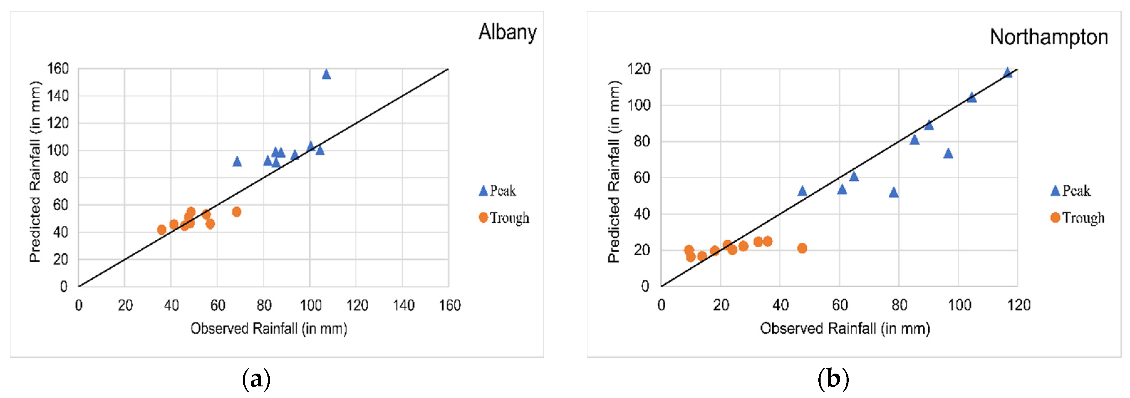
| Region | Rainfall Station | Peak | Trough |
|---|---|---|---|
| South Coast | Albany | 0.63 | 0.68 |
| Mount Barker | 0.90 | 0.57 | |
| Grassmere | 0.62 | 0.68 | |
| Busselton Shire | 0.52 | 0.43 | |
| North Coast | Northampton | 0.89 | 0.66 |
| Mingenew | 0.78 | 0.51 | |
| Nabawa | 0.77 | 0.63 | |
| Ogilvie | 0.78 | 0.60 |
| Author | Region | Rainfall | Method | Maximum Lagged Months | DMI–ENSO Model | |
|---|---|---|---|---|---|---|
| Pearson Correlation (r) | ||||||
| Calibration | Validation | |||||
| The current study (lagged) | WA | Autumn | ARIMAX | 4 | 0.56–0.82 | 0.62–0.80 |
| Islam and Imteaz [25] | WA | Autumn | MLR | 1 | 0.34–0.44 | 0.29–0.49 |
| Hossain, Rasel [61] | WA | Spring | MLR | 4 | 0.47–0.53 | 0.31–0.68 |
© 2020 by the authors. Licensee MDPI, Basel, Switzerland. This article is an open access article distributed under the terms and conditions of the Creative Commons Attribution (CC BY) license (http://creativecommons.org/licenses/by/4.0/).
Share and Cite
Islam, F.; Imteaz, M.A. Use of Teleconnections to Predict Western Australian Seasonal Rainfall Using ARIMAX Model. Hydrology 2020, 7, 52. https://doi.org/10.3390/hydrology7030052
Islam F, Imteaz MA. Use of Teleconnections to Predict Western Australian Seasonal Rainfall Using ARIMAX Model. Hydrology. 2020; 7(3):52. https://doi.org/10.3390/hydrology7030052
Chicago/Turabian StyleIslam, Farhana, and Monzur Alam Imteaz. 2020. "Use of Teleconnections to Predict Western Australian Seasonal Rainfall Using ARIMAX Model" Hydrology 7, no. 3: 52. https://doi.org/10.3390/hydrology7030052
APA StyleIslam, F., & Imteaz, M. A. (2020). Use of Teleconnections to Predict Western Australian Seasonal Rainfall Using ARIMAX Model. Hydrology, 7(3), 52. https://doi.org/10.3390/hydrology7030052