Abstract
Increased demand for engineering propositions to forecast rainfall events in an area or region has resulted in developing different rainfall prediction models. Interestingly, rainfall is a very complicated natural system that requires consideration of various attributes. However, regardless of the predictability performance, easy to use models have always been welcomed over the complex and ambiguous alternatives. This study presents the development of Auto–Regressive Integrated Moving Average models with exogenous input (ARIMAX) to forecast autumn rainfall in the South West Division (SWD) of Western Australia (WA). Climate drivers such as Indian Ocean Dipole (IOD) and El Nino Southern Oscillation (ENSO) were used as predictors. Eight rainfall stations with 100 years of continuous data from two coastal regions (south coast and north coast) were selected. In the south coast region, Albany (0,1,1) with exogenous input DMIOct–Nino3Nov, and Northampton (0,1,1) with exogenous input DMIJan–Nino3Nov were able to forecast autumn rainfall 4 months and 2 months in advance, respectively. Statistical performance of the ARIMAX model was compared with the multiple linear regression (MLR) model, where for calibration and validation periods, the ARIMAX model showed significantly higher correlations (0.60 and 0.80, respectively), compared to the MLR model (0.44 and 0.49, respectively). It was evident that the ARIMAX model can predict rainfall up to 4 months in advance, while the MLR has shown strict limitation of prediction up to 1 month in advance. For WA, the developed ARIMAX model can help to overcome the difficulty in seasonal rainfall prediction as well as its application can make an invaluable contribution to stakeholders’ economic preparedness plans.
1. Introduction
Long–term rainfall forecasting is one of the most challenging and demanding tasks. However, this is an important issue, which is directly related to the economy of a country. A reliable and accurate forecast can be beneficial for different authorities dealing with disaster management, water management, agricultural production, and flood management to set strategies, decision making, and taking precautionary measures before any natural calamities such as floods, drought, and bushfire could occur. Generally, two methods (statistical and dynamic modeling) have been used to forecast long–term rainfall [1]. A statistical method is less complex and requires less development time, but an uninterrupted and reliable data source is mandatory. On the other hand, the dynamic method is quite complex, requires more development time and expense [2,3]. Therefore, the application of statistical methods to forecast rainfall has become very popular among the researchers due to its simplicity, cost–effectiveness, and easy to implement characteristics. However, the use of the physically–based empirical model for seasonal rainfall prediction has also become popular since it overcomes the difficulties associated with conventional dynamic and statistical models [4,5].
At present, several time–series analyses are used as a statistical method for modeling and developing rainfall–runoff forecast models. Among them, the Auto–Regressive Integrated Moving Average (ARIMA) technique has become very popular due to its effective forecasting abilities over other conventional methods. Additionally, the ARIMA technique has shown effective results in terms of predicting the variability with better accuracy [6,7,8]. Over the years, several studies have considered ARIMA for developing rainfall forecasting models. Studies conducted by Brown, Kamruzzaman [9], Kamruzzaman, Beecham [10,11,12] have purposefully used the ARIMA technique to evaluate the trends and removing serial correlations in climate data. This is often termed as a ‘Pre–whitening Process’, that omits long term persistence of the climate variability, ensuring accurate trend identification and model construction [13,14,15]. Tularam [8] has used the ARIMA model for rainfall forecasting in Queensland, Australia, where the relationship between rainfall and temperature was investigated. Kumar, Soman [16] investigated climate variability and predictability of Indian summer rainfall using the ARIMA technique. Otok and Suhartono [17] developed a rainfall forecast model for Indonesia using the ARIMA method. Weeks and Boughton [18] have used the ARIMA model for rainfall–runoff prediction, while, Han, Wang [19] applied the ARIMA model for drought forecasting. Zhang [20] also developed a hybrid ARIMA and neural network model for forecasting.
The climate of Australia is mostly influenced by changes in sea surface temperature (SST) and sea level pressure (SLP) in nearby oceans. The mainland of Australia is surrounded by Pacific, Indian, and Southern oceans, therefore every climate driver generated from these oceans causes some impact on the Australian climate. Interestingly, the climate in different parts of Australia is influenced by unique climate characteristics that change differently with seasonal variation. The most unpredictable element of climate in Australia is its rainfall as different regions of Australia have different rainfall behaviors, such as coastal strips experience wetter winter compared to inland west. Many research studies were conducted that had an aim to explain rainfall variability throughout Australia [3,21,22,23,24]. Most of these research studies were primarily oriented toward the identification of climate indices responsible for rainfall variation and developing prediction models for such variability [3,8,23,25,26].
Rainfall variability has a great influence on Australian infrastructure, water resource system, agricultural production, crop, and flood management systems. Many research studies were conducted to investigate the Australian rainfall mechanism, and to understand this mechanism, researchers evaluated the relationships between climate indices and Australian seasonal rainfalls [3,23,26,27,28,29,30,31,32,33,34,35,36,37]. Past studies postulated that Australian rainfall largely varies with the interaction among climate drivers generated in Southern, Pacific, and Indian oceans [26,28,36]. However, their influences vary depending on the seasons and locations. Rainfall in different locations is controlled by different climate drivers generated around a specific region and more than one climate driver can be responsible for rainfall variability of a region.
The effect of El Nino Southern Oscillation (ENSO) in Australian rainfall is quite outstanding as it has been found as the most dominant driver compared to others. The effect of ENSO in the Australian climate is however debatable as it is unclear whether SST variation (Pacific or Indian) is responsible for such variability [21]. The generation of ENSO is a systematic tropical and extratropical response resulting from the movement of tropical convergence zones from their seasonal mean positions and this mechanism often develops in austral winter and spring and reaches its maximum during austral summer [38]. It was observed that ENSO has a significant correlation with Australian rainfall for at least one season, while the larger effect was found in eastern and north–eastern winter and spring rainfall [26]. Additionally, the effect of El Nino was found to be responsible for rainfall reduction in western and southern Australia during the winter period [28].
Indian Ocean Dipole (IOD) is an important contributor to rainfall variability in Australia and has a significant negative partial correlation with the western and southern Australian rainfall [39]. Although co–variation of sea surface temperature (SST) in the tropical Indian Ocean and that of the tropical Pacific exists, IOD itself can contribute to Australian inter–annual rainfall variability [40]. IOD is characterized by two phases, namely positive phase, and negative phase. During the positive phase, cold SST anomalies dominate the west of the Indonesian archipelago. It develops an anomalous anti–cyclonic circulation over much of the Australian continent and at lower levels over the eastern tropical and subtropical Indian Ocean. The negative phase just causes the opposite of the positive phase. According to Cai, Van Rensch [21], 79% of Australian rainfall occurred due to the negative phase of IOD while the positive phase works against the rainfall generation. The influence of IOD prevails from May to November and it reaches its peak during spring. IOD is also responsible for Western Australian rainfall from May to October [31]. Such physical attributes of IOD was also previously presented by Smith [41], who did refer to Drosdowsky and Williams [22], and McBride and Nicholls [24], reporting strongest correlations between IOD and rainfall over northern and south–eastern Australia during spring and weakest during autumn.
The combined effect of ENSO and IOD is also important for Australian rainfall. Both drivers are highly correlated with each other, which mostly prevails from June to October. Ashok, Guan [42] found that IOD and ENSO months are concurrently linked to each other as 27% from April to November, 21% from April to August, and 35% from September to November. This was supported by Risbey, Pook [26] as they denoted that the combined effect of ENSO and IOD are more extreme than either on their own, and it is difficult to separate their combined contribution to Australian rainfall events [43].
Specifically, the majority of the studies were mainly concentrated on evaluating correlations between Australian rainfalls and large scale climate indices [10,26,31]. However, a strong concurrent relationship does not always show the same relationship in lag. Hence lagged relationship study is more important compared to the concurrent relationship study, as forecasting is possible using the lagged relationships only. However, such an analysis requires more attention and precision during data preparation and analysis. Very few studies have been found which considered lagged relationships among Australian rainfalls and climate indices [3,29,44]. All these studies have adopted one or more of the following analysis: linear regression techniques [25,45,46], Bayesian modeling method [3], ARIMA [8,10], and artificial neural network (ANN) [46,47]. However, studies which have considered ARIMA techniques never included climate indices as predictors to develop rainfall forecasting model in Australia. Some researchers have successfully employed several different techniques such as adaptive neuro–fuzzy inference system (ANFIS), ANN, M5P Model Tree, multivariate adaptive regression splines (MARS), least squares support vector machine (LSSVM), classification and regression trees (CART) model for rainfall/streamflow forecasting in different parts of the world [48,49,50,51,52,53]. However, the effective independent variable(s) are unlikely to be the same for all regions, i.e., some climatic variable(s), which are effective for one part of the world are not necessarily to be effective for other parts. Additionally, a single technique may not produce the best results for the entire world. As such, it is necessary to investigate different techniques for a region, while focusing on the stakeholders’ needs. To satisfy such a requirement, a simple ARIMAX model was developed to predict autumn rainfall in WA and its prediction performance was compared with previously developed multiple linear regression (MLR) models for the same region. ARIMAX model has been selected due to its superiority in terms of prediction performance over ARIMA and other models [54,55,56,57]. A study conducted by Jalalkamali [58] reported that forecasting using ARIMAX is possible with 9 months lagged period whereas the performance has been as outstanding if compared to multilayer perceptron artificial neural network (MLP–ANN), support vector machine (SVM) models, and adaptive neuro–fuzzy inference systems (ANFIS) models. Considering such facts, the ARIMAX model could produce much necessary flexibility required to meet the stakeholder’s needs.
2. Data and Study Area
This study aims to predict WA autumn rainfall using potential climate indices as predictors. Autumn comprises of the months: March–April–May, while the weather becomes more favorable for preparing seedlings, hence, a season of great importance for farmers and stakeholders. A good prediction of autumn rainfall can help the farmers in decision making for potential crop yields and making economic adjustments, thus, setting economic preparedness plans. Therefore, having a reliable autumn rainfall forecast model is expected to benefit the stakeholders and policymakers to take precise decisions at critical times. To reach the aim of the study, SWD of WA was selected as potential sites as more than 80% of the total Western Australian population live here as well as 80% of WA exportable goods grow in this region (refer to Figure 1).
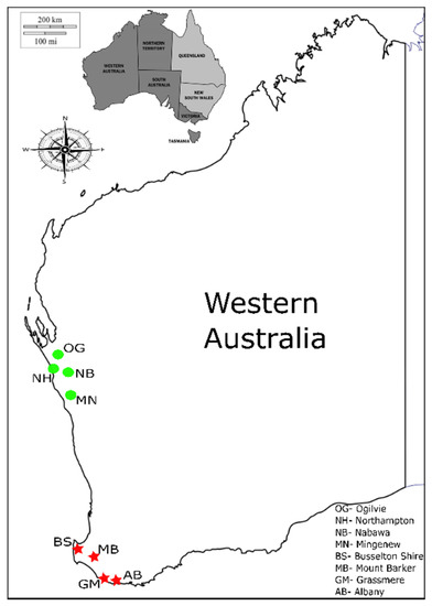
Figure 1.
Map and location of selected rainfall stations in Western Australia.
To conduct this study, monthly rainfall data and climate index data were collected for eight different stations located in two different regions. The monthly rainfall data was retrieved from the Australian Bureau of Meteorology website (www.bom.gov.au/climate/data/) and climate index data was collected from the climate explorer website (http://climexp.knmi.nl/). All the rainfall stations were in the south–west division of WA and for each station, 100–years continuous rainfall data was collected. The location, description, and seasonal rainfall data for Summer (Dec–Jan–Feb), Autumn (Mar–Apr–May), Winter (Jun–Jul–Aug), and Spring (Sep–Oct–Nov) for these stations is presented in Table 1.

Table 1.
Geographical location and description of rainfall stations.
Past studies suggest that climate indices namely, Dipole Mode Index (DMI), Nino3, Nino3.4, Nino4, Southern Oscillation Index (SOI), Southwest Australian Circulation (SWAC), Southern Annular Mode (SAM), and ENSO Modoki Index (EMI) cause influence on Western Australian rainfall [26,33,36,59]. For this study, Nino3, Nino3.4, Nino4, SOI, EMI, and DMI were selected as potential climate indices due to the availability of 100 years of continuous data. However, SWAC and SAM were excluded from the analyses due to the non–availability of long–term continuous data.
All the climate indices have a complex but interesting formation mechanism. ENSO is measured by two types of indicators; SOI, which is the measure of Sea Level Pressure (SLP) difference between Darwin and Tahiti; and the rest are Nino3.4, Nino3, and Nino4. Nino3.4 is the average Sea Surface Temperature (SST) anomalies in the western pacific bounded by 5° N to 5° S, from 170° W to 120° W; Nino3 is the average SST anomalies in the eastern pacific bounded by 5° S–5° N, from 90° W–150° W; and Nino4 is the average SST anomalies in central pacific bounded by 5° N to 5° S, from 150° W to 160° E [26]. The EMI is the difference between El–Nino and traditional events, which have maximum warming in central Pacific and eastern Pacific, respectively. It is expressed by the following equation: EMI = SST_X − 0.5*SST_Y − 0.5*SST_Z (Here, X = 165° E–140° W, 10° S–10° N, Y = 110° W–70° W, 15° S–5° N, Z = 125° E–145° E, 10° S–20° N) [60]. DMI is the indicator of IOD, which is defined as the average SST anomalies between tropical western Indian Ocean bounded by 10° N to 10° S, from 50° E to 70° E and the tropical south–eastern Indian Ocean bounded by 110°S to the equator from 90° E to 110° E [40].
3. Methodology
In this study, Time Series Analysis was used to develop forecasting models. Among various time series methods, ARIMA method has become very popular. For time series analysis, two types of ARIMA methods are mostly used: univariate ARIMA and multivariate ARIMA or transfer function model. In an ARIMA model, the inclusion of exogenous variable (predictors) or explanatory variables is termed as ARIMAX model [15]. In the ARIMAX model, ARIMA orders for dependent variables while transfer function orders for independent variables or predictors. Using ARIMAX model in particular, Kamruzzaman, Beecham [12] have illustrated a detailed way of including predictors, the possible number of predictors, and how the inclusion of the past value of climate indices can improve the forecasting ability. In this study, the ARIMAX model was used for the prediction of Western Australian autumn rainfall, where large–scale climate indices were used as independent variables. 100 years of data were split into two periods: the calibration period (1916–1985) and the validation period (1986–2015). Collected monthly rainfall data was then converted into seasonal autumn rainfall (Australian standard autumn months: March–April–May) data and climate indices data was collected and accumulated for the preceding months to perform analysis with lagged climate indices. Bivariate correlation was performed to select significant independent variables which were later included as transfer functions to develop the ARIMAX model. Results of the ARIMAX model were evaluated using standard statistical test parameters, profoundly used in past studies [46,47,61,62,63]. These include Pearson correlation coefficient (r), root mean square error (RMSE), mean absolute percentage error (MAPE), mean absolute error (MAE), normalized Bayesian information criterion (BIC), and refined Willmot index of agreement () values. Additionally, ARIMAX produced results were compared with the results of multiple linear regression (MLR) analysis which were performed earlier in different investigations [25,61]. All these analyses were performed in the IBM SPSS Statistics 26 software package.
3.1. Multivariate Auto–Regressive Integrated Moving Average with Exogenous Input (ARIMAX)
ARIMA model is composed of ‘AR’, ‘I’, and ‘MA’ where ‘AR’ stands for Auto–Regressive, ‘I’ is for Integrated, a time series which needs to be differenced to make a non–stationary series to stationary, ‘MA’ stands for Moving Average. The general expression of the ARIMA model is ARIMA (p, d, q) *(P, D, Q). This contains two parts: one is non–seasonal and the other one is seasonal, where, (p, d, q) is the non–seasonal part, and (P, D, Q) is the seasonal part. Here, ‘p’ denotes non–seasonal auto–regressive order, ‘d’ denotes non–seasonal differencing, ‘q’ denotes non–seasonal moving average, whereas, ‘P’ denotes seasonal auto–regressive order, ‘D’ denotes seasonal differencing, and ‘Q’ denotes seasonal moving average. In this study, the time–series show no seasonality, therefore, only the non–seasonal part was used. In the ARIMAX model, two types of input orders are required: one is ARIMA order (dependent variable; autumn rainfall) and the other is transfer function order (predictors or independent variable; climate indices) [64]. A description of these input orders are presented as follows:
ARIMA Order (p, d, q):
- Autoregressive (p): it is defined as the number of autoregressive orders in the model. Autoregressive orders specify which previous values from the series are used to predict the present values.
- Difference (d):it is defined as the order of differencing in the model. Differencing is necessary to make a non–stationary series into stationary series. As the ARIMA model is stationary, it is necessary to remove the non–stationary effects before estimating models. A first–order differencing is often proved as enough for linear trends, while a second–order differencing is required for quadratic trend.
- Moving Average (q): it is defined as the number of moving average orders in the model. Moving average orders specify how deviation from the series mean of previous values (past errors) is used to predict current values. Therefore, it is the number of lagged forecast errors in the predicted equation.
Therefore, for example, a model described as ARIMA (0,1,1) refers to containing zero auto–regressive (p) and one moving average (q) parameters with the first order of differencing (d) of the data.
Transfer Function Orders:
Transfer function order specifies which past values of independent variables are used to predict future values of dependent series.
- Numerator: it is the number of orders of the numerator in the transfer function. It states which past values of independent series are used to predict the current value of the dependent series. Such as a numerator value of 1 states that the one–time period past value and the current value of an independent series are used to predict the current values of the dependent series.
- Denominator: it is the number of orders of the denominator in the transfer function. It is specified to predict the current value of the dependent series and how deviations from the series mean for previous values of independent variables are used. For instance, a denominator number of 1 indicates that the deviation from the mean of the independent series one period in the past is considered to predict the current values of the dependent series.
- Difference: it is the order of differencing. It is applied to make a non–stationary series into stationary before estimating the model.
An elaborative formation of the ARIMAX model equation has been discussed and presented in Box, Jenkins [65], and Hamilton [66]. The ARIMAX (p, d, q) model equation for time series and exogeneous data is presented below in Equation (1):
where, φ1, …, φp and θ1, …, θq are the parameters; εt, εt−1 are white noise error and β1, …, βm are the parameters of independent variables input Xt and t is the time.
ARIMAX model consists of three steps [19,65,67]:
- Identification: in this stage, first, the raw data series is plotted to identify whether the data is stationary or not. If the raw data series is found to be non–stationary, differencing is required. After the first order differencing, correlograms of the autocorrelation function (ACF) and partial autocorrelation function (PACF) is investigated. From these plots, the order of AR and MA gets identified.
- Parameter Estimation and Selection: the number of AR depends on the lag of PACF cuts and the number of MA depends on the lag of the ACF plot. However, decision making on the order of AR and MA by looking at the cuts/spikes is not straightforward. Most of the time it required experimentation with several alternative orders of different models to choose the appropriate order. The following guidelines are usually followed during the selection of the AR and MA order:
- If the ACF plot shows exponential decay and PACF spikes at lag–1, no correlation for other lags, in that case, one autoregressive parameter (p = 1) can be selected.
- If the ACF plot shows a sine–wave shape pattern or a set of exponential decay and PACF spikes at lag–1 and lag–2, no correlation for other lags, in that case, two autoregressive parameters (p = 2) can be selected.
- If the PACF plot shows exponential decay and ACF spikes at lag–1, no correlation for other lags, in that case, one moving average parameter (q = 1) can be selected.
- If the PACF plot shows a sine–wave shape pattern or a set of exponential decay and ACF spikes at lag–1 and lag–2, no correlation for other lags, in that case, two moving average parameters (q = 2) can be selected.
- One auto–regressive and one moving average parameter can be selected if both shows exponential decay starting at lag–1.
- Sometimes, using both AR and MA orders in a model can cancel each other’s impact. Therefore, it is often wise to use mixed AR and MA models with less number of orders.
- Diagnostics Check: the diagnostic check is required to verify the adequacy of the developed model. The residual of the developed model should be white noise (no autocorrelation). To check whether the residual is white noise or not, at first, an inspection of the residual ACF and PACF plot is required. If 95% of the spikes stay between the black lines, it indicates that the autocorrelation is white noise. If two or more spikes or more than 5% of spikes are located outside of the boundary line, then the series is not white noise. Another way of checking the model accuracy is to perform the Ljung–Box test. Such a test is conducted to verify the null hypothesis of being white noise of residual if the p–value is greater than 0.05 [68]. A p–value greater than 0.05 implies that lag autocorrelation among the residuals is zero and the developed model is adequate to fit the data set.
3.2. Statistical Parameters for ARIMAX Model
Among all the statistical parameters that were used to evaluate the ARIMAX model’s performance, RMSE calculates prediction errors, the measure of how much a dependent series varies from its model–predicted level. MAE is the average of the absolute errors/residuals between observed and predicted value, while MAPE is the measure of prediction accuracy of a developed model. It is also known as the mean absolute percentage deviation. For both RMSE and MAE, a value of 0 indicates a perfect predictability performance. Thus, the lower the value of RMSE, MAE, and MAPE the better is the model’s performance [69,70]. The equation for RMSE, MAE, and MAPE is presented in Equations (2)–(4):
where is the observed value, is the predicted value and n is the number of observations.
Normalized Bayesian information criterion (BIC) is the measure of the overall fit of the developed model. It measures the model’s complexity based on mean square error, the number of parameters, and series length. A lower value indicates a low complexity of the model and reverses for the higher value. Thus, a model with a lower BIC is always preferred.
However, all these tests have some shortcomings, which can be overruled by the introduction of a refined index of agreement () developed by Willmott [71]. ‘’ is the reformulation of Willmott’s index of agreement (d). It specifies the sum of the magnitudes of the differences between the predicted and observed deviations from the observed mean relative to the sum of the magnitudes of the perfect model (, for all i) and observed deviations from the observed mean. The refined index of agreement () can be calculated using the following Equation (5):
where is the predicted value of the ith observation, is the observed value of the ith observation, is the observed mean value, and n is the sample size. c value equals 2 as suggested in the equation.
A value of = 0.5 indicates that the sum of the error magnitude is one half (0.5) of the sum of the perfect model deviation and observed model deviation magnitude. Besides, the value of = 0.0 indicates the sum of the magnitude of the errors, and the sum of the perfect model and the observed deviation magnitudes are equal. Moreover, the value of = −0.5 indicates the sum of the error magnitudes is twice the sum of the perfect model and the observed deviation magnitudes. For ‘’, a positive value indicates a good fit, while a negative value indicates complete disagreement.
4. Results
Eight rainfall stations from two coastal regions, namely, South Coast and North Coast in WA were selected to conduct this study. Lagged monthly climate indices values (Junen−1 to Febn) were used to investigate the correlation with autumn rainfall (March–April–May). Here, ‘n’ is the predicted year, and ‘n – 1’ is the previous year. At first, Bivariate correlation analysis was conducted to determine the significant correlation between rainfall and climate indices. Table 2 presents the bivariate correlation results for the selected rainfall stations.

Table 2.
Pearson correlation (r) between lagged climate indices and autumn rainfall.
Climate indices, which showed a significant correlation (r) were used as a predictor in the ARIMAX technique. Past studies have shown that a combination of two or more climate indices has improved forecasting ability [26,72]. Therefore, from earlier correlation analysis, a combination of influential climate indices was used as exogenous variables (Predictors) in ARIMAX modeling.
Once significant climate indices were selected, stationarity and seasonality of the data were assessed. In the identification stage, both rainfall and climate index data were found as non–stationary and rainfall pattern was found as non–seasonal. To make the data stationary, a first–order differencing was performed on both rainfall and climate indices data. Differencing was kept limited until first–order only as it deemed sufficient for any linear trend [64]. For the station Albany, Figure 2 depicts the non–stationary and stationary state of rainfall data before and after first order differencing, while Figure 3 and Figure 4 illustrate the same for associated climate indices. A similar strategy has been followed for other stations analyzed in this study.
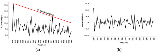
Figure 2.
Rainfall data for Albany: (a) before differencing and (b) after differencing.

Figure 3.
Climate indices DMIOct for Albany: (a) before differencing and (b) after differencing.

Figure 4.
Climate Indices Nino3Nov for Albany: (a) before differencing and (b) after differencing.
The next step involved parameter estimation, where AR and MA order was selected from the PACF and ACF plots of selected rainfall stations. PACF plot was used to select AR order, while the ACF plot was used to select MA order. Figure 5 presents ACF and PACF plots with respective lag numbers for the station Albany.

Figure 5.
(a) Autocorrelation function (ACF) plot of rainfall in Albany and (b) partial autocorrelation function (PACF) plot of rainfall in Albany.
From Figure 5a, it can be observed that the ACF plot contains only one spike located outside of the confidence limit, while the rest are close to zero. On the other hand, in Figure 5b, in the PACF plot, exponential decay is evident with four spikes being present outside the confidence limit. Considering such facts, ARIMAX (0,1,1) was selected for Albany. For the remaining rainfall stations, a similar strategy was followed to select the appropriate AR and MA orders. For most of the rainfall stations, ARIMAX (0,1,1) model was found as most suitable except two stations (Mount Barker and Busselton Shire). ARIMA orders and transfer function orders for all these stations are presented in Table 3 and Table 4. The insertion of ARIMAX criteria for model and transfer functions is presented in Appendix A, Figure A1.

Table 3.
ARIMA model input.

Table 4.
Transfer function input.
Several ARIMAX models were developed using different combinations such as DMI–Nino3, DMI–Nino4, DMI–Nino3.4, DMI–SOI, and DMI–EMI for both the south coast and north coast regions. Table 5 presents the total outcome of a combination set of different models.

Table 5.
Pearson correlation (r) results with the different model sets in ARIMAX.
Table 5 illustrates that the DMI–Nino3 model shows the highest significant correlations (r) for all rainfall stations in both regions. For Albany, the DMI–SOI model showed the highest correlation (r), however, the DMI–Nino3 model showed a consistently better correlation for all other stations. Thus, the DMI–Nino3 model was selected as the best model. Table 6 presents the statistical performance of the developed DMI–Nino3 models for selected rainfall stations.

Table 6.
Model description of the selected ARIMAX models in the calibration period.
Once the ARIMAX model got developed, a diagnostic check was performed to check the adequacy of the model. A Ljung–Box test was conducted to check the residuals, whether these are white noise or not. For all these developed models, the associated p–values are found to be greater than 0.05, which holds the null hypothesis of being white noise [68]. Another alternative way of checking the residual autocorrelation is to draw residual ACF and PACF plots as presented in Figure 6. Figure 6 demonstrates that all the spikes are located within the black boundary lines, depicting that no autocorrelation among the residuals exist. Similar results were found for other rainfall stations (refer to Appendix A, Figure A2).
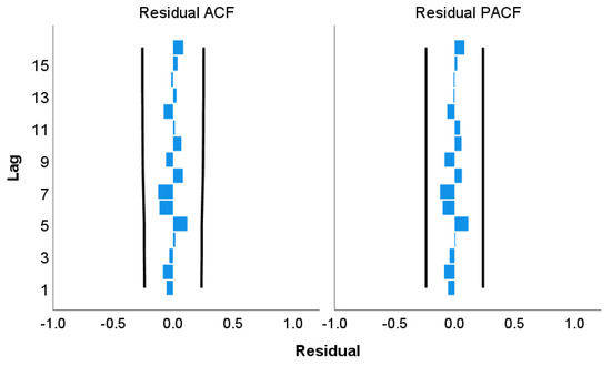
Figure 6.
Residual ACF and PACF plot for Albany.
A validation test was performed with the same model input sets using ARIMAX analysis. In the validation period, the developed model showed an increased correlation (r) compared to the calibration period for all stations except Mount Barker, Northampton, and Nabawa. Refined Willmott index of agreement () was also calculated for both calibration and validation periods. Based on the correlation and refined index of agreement statistics, a detailed comparison between the developed ARIMAX model and previously developed MLR models were made and presented in Table 7. From Table 7, it is observed that the ARIMAX model showed significantly higher correlations (0.56–0.82), compared to the MLR model (0.34–0.44) in the calibration period. For Albany and Northampton, the prediction performance of the ARIMAX and MLR model is presented in Figure 7. Similar plots for other stations are also presented in Appendix B, Figure A3.

Table 7.
Pearson correlation (r) and refined index of agreement () in the calibration and validation period for the ARIMAX and multiple linear regression (MLR) model
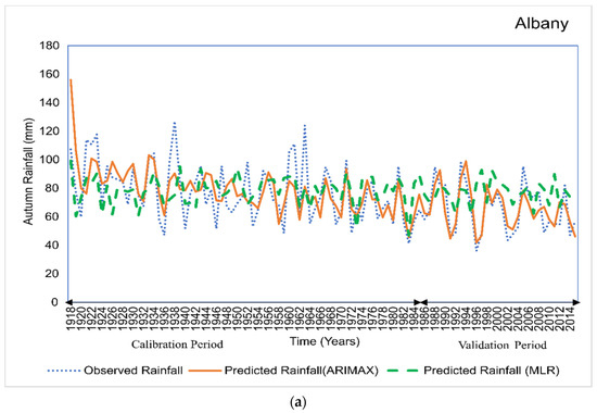
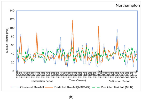
Figure 7.
Prediction performance of the developed models for (a) Albany and (b) Northampton.
To evaluate the ARIMAX model’s performance to capture extreme cases, peak and trough analysis was performed. The correlation coefficients (r) between observed and predicted peak and trough values for selected rainfall stations are presented in Table 8. The DMI–Nino3 model has shown its capability of capturing peaks with a correlation of 0.52–0.90, and 0.77–0.89 on the south coast and north coast, respectively. In contrast, for the trough, the correlation ranged from 0.43 to 0.68, and 0.51 to 0.66, respectively. Peak and trough plots for the station Albany and Northampton are presented in Figure 8, while similar plots for other stations are presented in Appendix B, Figure A4.

Table 8.
Correlation coefficients (r) between observed and predicted peak and trough values.
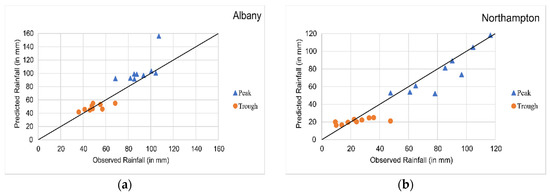
Figure 8.
Peak and trough detection using ARIMAX model for (a) Albany and (b) Northampton.
Finally, a comparative evaluation of previously developed models for WA was performed. A summary of the comparison is presented in Table 9.

Table 9.
Pearson correlation (r) between combined climate indices and Western Australian rainfall.
The comparison made above (refer to Table 9) suggests that high Pearson correlation (r) values were obtained in the ARIMAX model, referring to its superiority over multiple linear regression (MLR) models. ARIMAX model was also found as more favorable due to its 4 months lagged prediction capability.
5. Discussion
This paper presents the inclusion of exogenous variables in the ARIMA model (termed as ARIMAX) and showed good prediction performance for WA rainfall variability. The inclusion of an exogenous variable is only possible if these predictors show a significant correlation with the dependent variable [64]. Correlation analyses were conducted between single climate index and autumn rainfall to identify statistically significant climate index for selected rainfall stations in WA. Except for EMI, all the selected climate indices showed low to medium Pearson correlation (r) with autumn rainfall in 5 months lagged period (October to February). However, EMI showed a significant correlation only for north coast rainfall stations that aligns with the findings of Taschetto and England [59]. SST based climate indices (Nino3.4, Nino3, and Nino4) showed a better correlation (r) compared to SLP based index (SOI). This has also been consistent with the findings of Drosdowsky and Chambers [29], where they showed SOI has less predictability skill for Western Australian autumn rainfall compared to SST indices with 1–3 months lag period.
Several ARIMAX models were developed using a combination of different significant climate indices. Model sets were developed with lagged DMI–Nino3, lagged DMI–Nino4, lagged DMI–Nino3.4, lagged DMI–SOI, and lagged DMI–EMI for both the south coast and north coast regions. All the model sets and their Pearson correlation (r) are presented in Table 5, from where the DMI–Nino3 model was selected as the best model for both the regions.
The statistical performance parameters for the selected DMI–Nino3 model are presented in Table 6, wherein the calibration period, the Pearson correlation (r) for the rainfall magnitudes ranged from a minimum of 0.58 to a maximum of 0.67 in the south coast region. These developed models can predict seasonal autumn rainfall for 4 months in advance for the region. Similarly, for the north coast region, Pearson correlation (r) ranged from 0.56 to 0.82 in the calibration period. The station Mingenew and Northampton predicted seasonal autumn rainfall for 4 months and 2 months in advance. The remaining two stations, namely Nabawa and Ogilvie, showed the prediction for 1 month in advance only. Such capability of the model to predict up to 6 months in advance has also been justified in several past studies [3,24,46,47,61,73]. All these studies considered lagged climate indices to forecast Australian seasonal rainfall as the current study did. Schepen, Wang [3] conducted a study on the evidence of using lagged climate indices for forecasting Australian seasonal rainfall using one climate index. It has shown positive evidence to use climate indices to predict rainfall in several months advance (1–3 months or one season). A study conducted by Abbot and Marohasy [47] used artificial neural network (ANN) with 1–3 months lagged period input parameters. The finding of their study depicted that the monthly forecast in 3 months in advance is as skillful as 1 month in advance. Similar attempts made by Mekanik, Imteaz [46], Ghamariadyan, Imteaz [73], Rasel, Imteaz [35] showed that seasonal rainfall forecast can be possible from 3 to 6 months in advance for different regions in Australia.
The developed ARIMAX models for both south coast and north coast regions have also shown low values of RMSE, MAPE, MAE, and normalized BIC values (refer to Table 6). Low values of all these parameters indicate a good prediction performance of the developed models. Once the models were developed for the calibration period, validation tests were performed with the same model input sets using ARIMAX analysis (refer to Table 7). In the validation period, the developed model showed an increased correlation (r) compared to the calibration period for all stations except Mount Barker, Northampton, and Nabawa. For the south coast region, Albany showed the highest correlation (r) value of 0.60 in calibration and 0.80 in the validation period with a lag of 4 months. In contrast, for the north coast region, Northampton showed the highest Pearson correlation (r) value of 0.82 in calibration and 0.70 in the validation period with a lag of 2 months. Statistically, a Pearson correlation (r) value greater than 0.5 indicates a large effect [74]. A similar observation was made for Refined Willmott index of agreement (), where the ‘’ value was over 0.60 for all the stations, except for Mingenew. In both calibration and validation periods, the highest value of ‘’ was reported for Albany on the south coast and Northampton on the north coast, respectively. Since all the stations depicted positive higher values of ‘’, this indicates a good fit of the model [71].
To understand the effectiveness of the ARIMAX model, its statistical performance parameters were compared with previously developed MLR models for the same regions. From such comparison, a significant rise in Pearson correlation (r) values was observed in ARIMAX models for both calibration and validation periods. An increase in ‘’ values was also obtained for the ARIMAX models. Moreover, MLR models showed relatively poor prediction performance with only 1 month lag, whereas the ARIMAX models showed better prediction with 4 months lag. In terms of reliability, ARIMAX outperformed its MLR counterparts with better efficiency and accuracy. Furthermore, ARIMAX models successfully captured some of the extreme events, and followed the same rainfall trend as observed rainfall, whereas, the MLR models failed to do so (refer to Figure 7). The finding of this study reinforced ARIMAX models’ superiority over MLR models. Many past studies also emphasized ARIMAX models’ superiority over other modeling approaches [54,55,56,57,58].
6. Conclusions
This study investigated the influence of climate drivers on Western Australian rainfall variability and developed a forecast model to predict seasonal autumn rainfall using the ARIMAX technique. In this attempt, climate drivers were used as transfer functions, while all other previous attempts considered conventional time series models only. From a statistical perspective, it was evident that the predictability performance of the ARIMAX model is much higher than the MLR models. The ARIMAX models are capable of predicting rainfall 4 months in advance while the conventional MLR model can predict the rainfall only 1 month in advance. The developed ARIMAX models have shown a strong correlation (r) as well as minimum errors, smaller BIC values, and higher refined index of agreement values () in both calibration and validation periods, depicting the model’s non–erroneous prediction capability. It was also observed that all these ARIMAX models were successful in predicting some of the extreme rainfall events and droughts, while their ability to predict seasonal autumn rainfall in advance of 4 months has strengthened their acceptability. From the stakeholder’s perspective, such flexibility offered in the developed model has greater importance, as a timely prediction can help in strategic decision making and reducing associated risks and damage potentials. Overall, the DMIOct–Nino3Nov model for the south coast and DMIJan–Nino3Nov model for the north coast showed exceptional performance with good prediction accuracy and can be recommended for future rainfall prediction in WA. However, the developed models have some limitations as they were not able to predict all extreme cases. Investigating the existing nonlinear relationship between rainfall and climate drivers can provide a better understanding of the trend, and associated variabilities that the developed models failed to address. Possible analysis approaches can be considered for developing nonlinear models and hybrid models. Since rainfall is a complex mechanism, any linear or nonlinear model by itself, might not be able to predict or capture all the extreme cases. For such instances, a hybrid model could offer a better solution. The ARIMAX model residuals can be used to explain the nonlinear relationships, where the combined output of both ARIMAX and non–linear models can be used for improved forecasting.
Author Contributions
F.I. was involved in methodology development, data curation, formal analysis, investigation, software use, validation, writing—original draft preparation. M.A.I. was involved in conceptualization, resources allocation, supervision, project administration, and writing—review and editing. All authors have read and agreed to the published version of the manuscript.
Funding
This research received no external funding.
Acknowledgments
The first author acknowledges the Australian government’s “Research Training Program (RTP) Fees Offset Scholarship” for studying at Swinburne University of Technology, Melbourne.
Conflicts of Interest
The authors declare no conflict of interest.
Appendix A
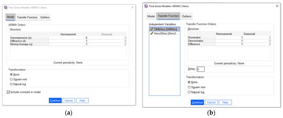
Figure A1.
ARIMAX input for (a) model and (b) transfer functions.
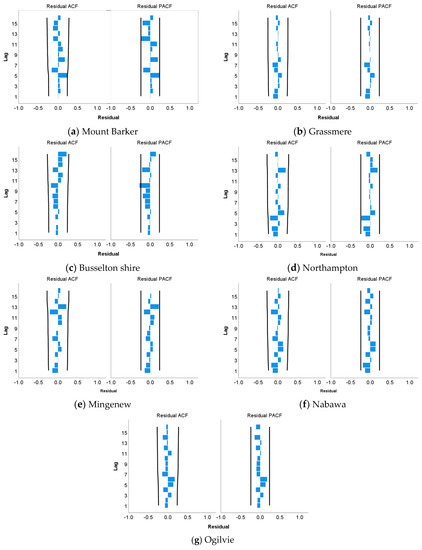
Figure A2.
Residual ACF and PACF plot for (a) Mount Barker; (b) Grassmere; (c) Busselton Shire; (d) Northampton; (e) Mingenew; (f) Nabawa; (g) Ogilvie.
Appendix B
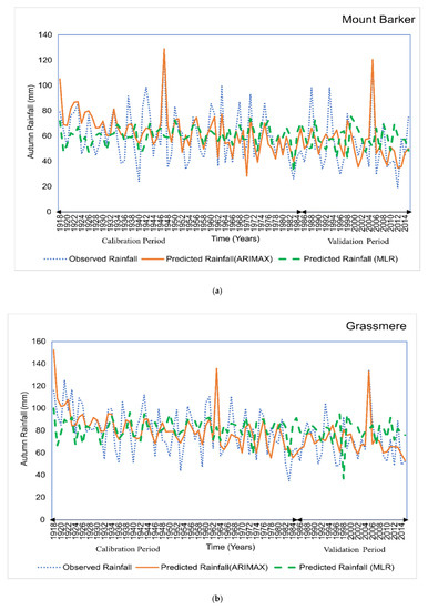
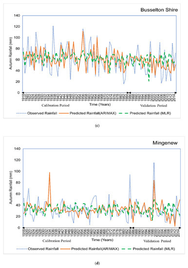
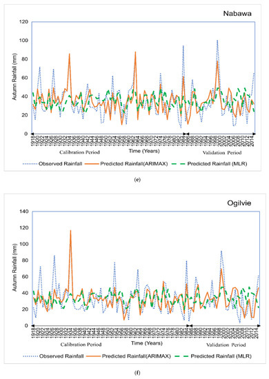
Figure A3.
Prediction performance of the developed models for (a) Mount Barker; (b) Grassmere; (c) Busselton Shire; (d) Mingenew; (e) Nabawa; (f) Ogilvie.
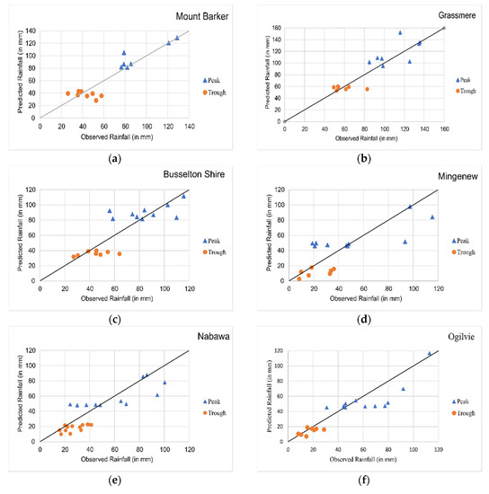
Figure A4.
Peak and trough detection using ARIMAX model for (a) Mount Barker; (b) Grassmere; (c) Busselton Shire; (d) Mingenew; (e) Nabawa; (f) Ogilvie.
References
- Goddard, L.; Mason, S.J.; Zebiak, S.E.; Ropelewski, C.F.; Basher, R.; Cane, M.A. Current approaches to seasonal to interannual climate predictions. Int. J. Climatol. 2001, 21, 1111–1152. [Google Scholar] [CrossRef]
- Anderson, J.; van den Dool, H.; Barnston, A.; Chen, W. Present-day capabilities of numerical and statistical models for atmospheric extratropical seasonal simulation and prediction. Bull. Am. Meteorol. Soc. 1999, 80, 1349–1362. [Google Scholar] [CrossRef]
- Schepen, A.; Wang, Q.; Robertson, D. Evidence for using lagged climate indices to forecast Australian seasonal rainfall. J. Clim. 2012, 25, 1230–1246. [Google Scholar] [CrossRef]
- Li, J.; Wang, B. Origins of the decadal predictability of East Asian land summer monsoon rainfall. J. Clim. 2018, 31, 6229–6243. [Google Scholar] [CrossRef]
- Li, J.; Wang, B.; Yang, Y.M. Retrospective seasonal prediction of summer monsoon rainfall over West Central and Peninsular India in the past 142 years. Clim. Dyn. 2017, 48, 2581–2596. [Google Scholar] [CrossRef]
- Momani, P.; Naill, P. Time series analysis model for rainfall data in Jordan: Case study for using time series analysis. Am. J. Environ. Sci. 2009, 5, 599. [Google Scholar] [CrossRef]
- Mondal, P.; Shit, L.; Goswami, S. Study of effectiveness of time series modeling (ARIMA) in forecasting stock prices. Int. J. Comput. Sci. Eng. Appl. 2014, 4, 13. [Google Scholar] [CrossRef]
- Tularam, G. Relationship between El Niño southern oscillation index and rainfall (Queensland, Australia). Int. J. Sustain. Dev. Plan. 2010, 5, 378–391. [Google Scholar] [CrossRef]
- Brown, K.; Kamruzzaman, M.; Beecham, S. Trends in sub-daily precipitation in Tasmania using regional dynamically downscaled climate projections. J. Hydrol. Reg. Stud. 2017, 10, 18–34. [Google Scholar] [CrossRef]
- Kamruzzaman, M.; Beecham, S.; Metcalfe, A. Climatic influences on rainfall and runoff variability in the southeast region of the Murray-Darling Basin. Int. J. Climatol. 2013, 33, 291–311. [Google Scholar] [CrossRef]
- Kamruzzaman, M.; Beecham, S.; Metcalfe, A. Estimation of trends in rainfall extremes with mixed effects models. Atmos. Res. 2016, 168, 24–32. [Google Scholar] [CrossRef]
- Kamruzzaman, M.; Beecham, S.; Metcalfe, A.V.; Cai, W. Granger causal predictors for maximum rainfall in Australia. Atmos. Res. 2019, 218, 1–11. [Google Scholar] [CrossRef]
- Bloomfield, P. Trends in global temperature. Clim. Chang. 1992, 21, 1–16. [Google Scholar] [CrossRef]
- Cohn, T.A.; Lins, H.F. Nature’s style: Naturally trendy. Geophys. Res. Lett. 2005, 32, L23402. [Google Scholar] [CrossRef]
- Kamruzzaman, M.; Metcalfe, A.V.; Beecham, S. Wavelet-based rainfall–stream flow models for the southeast Murray darling basin. J. Hydrol. Eng. 2013, 19, 1283–1293. [Google Scholar] [CrossRef]
- Kumar, K.K.; Soman, M.; Kumar, K.R. Seasonal forecasting of Indian summer monsoon rainfall: A review. Weather 1995, 50, 449–467. [Google Scholar] [CrossRef]
- Otok, B.W.; Suhartono, F. Development of rainfall forecasting model in Indonesia by using ASTAR, transfer function, and ARIMA methods. Eur. J. Sci. Res. 2009, 38, 386–395. [Google Scholar]
- Weeks, W.; Boughton, W. Tests of ARMA model forms for rainfall-runoff modelling. J. Hydrol. 1987, 91, 29–47. [Google Scholar] [CrossRef]
- Han, P.; Wang, P.X.; Zhang, S.Y.; Zhu, D.H. Drought forecasting based on the remote sensing data using ARIMA models. Math. Comput. Model. 2010, 51, 1398–1403. [Google Scholar] [CrossRef]
- Zhang, G.P. Time series forecasting using a hybrid ARIMA and neural network model. Neurocomputing 2003, 50, 159–175. [Google Scholar] [CrossRef]
- Cai, W.; van Rensch, P.; Cowan, T.; Hendon, H.H. Teleconnection pathways of ENSO and the IOD and the mechanisms for impacts on Australian rainfall. J. Clim. 2011, 24, 3910–3923. [Google Scholar] [CrossRef]
- Drosdowsky, W.; Williams, M. The Southern Oscillation in the Australian region. Part I: Anomalies at the extremes of the oscillation. J. Clim. 1991, 4, 619–638. [Google Scholar] [CrossRef]
- Kirono, D.G.; Chiew, F.H.; Kent, D.M. Identification of best predictors for forecasting seasonal rainfall and runoff in Australia. Hydrol. Process. 2010, 24, 1237–1247. [Google Scholar] [CrossRef]
- McBride, J.L.; Nicholls, N. Seasonal relationships between Australian rainfall and the Southern Oscillation. Mon. Weather Rev. 1983, 111, 1998–2004. [Google Scholar] [CrossRef]
- Islam, F.; Imteaz, M.A. Development of prediction model for forecasting rainfall in Western Australia using lagged climate indices. Int. J. Water 2019, 13, 248–268. [Google Scholar] [CrossRef]
- Risbey, J.S.; Pook, M.J.; McIntosh, P.C.; Wheeler, M.C.; Hendon, H.H. On the remote drivers of rainfall variability in Australia. Mon. Weather Rev. 2009, 137, 3233–3253. [Google Scholar] [CrossRef]
- Chiew, F.H.; Piechota, T.C.; Dracup, J.A.; McMahon, T.A. El Nino/Southern Oscillation and Australian rainfall, streamflow and drought: Links and potential for forecasting. J. Hydrol. 1998, 204, 138–149. [Google Scholar] [CrossRef]
- Chowdhury, R.K.; Beecham, S. Influence of SOI, DMI and Niño3. 4 on South Australian rainfall. Stoch. Environ. Res. Risk Assess. 2013, 27, 1909–1920. [Google Scholar] [CrossRef]
- Drosdowsky, W.; Chambers, L.E. Near-global sea surface temperature anomalies as predictors of Australian seasonal rainfall. J. Clim. 2001, 14, 1677–1687. [Google Scholar] [CrossRef]
- Feng, J.; Li, J.; Li, Y. Is there a relationship between the SAM and southwest Western Australian winter rainfall? J. Clim. 2010, 23, 6082–6089. [Google Scholar] [CrossRef]
- Fierro, A.O.; Leslie, L.M. Links between central west Western Australian rainfall variability and large-scale climate drivers. J. Clim. 2013, 26, 2222–2246. [Google Scholar] [CrossRef]
- Marshall, A.; Hendon, H. Impacts of the MJO in the Indian Ocean and on the Western Australian coast. Clim. Dyn. 2014, 42, 579–595. [Google Scholar] [CrossRef]
- Montazerolghaem, M.; Vervoort, W.; Minasny, B.; McBratney, A. Long-term variability of the leading seasonal modes of rainfall in south-eastern Australia. Weather Clim. Extrem. 2016, 13, 1–14. [Google Scholar] [CrossRef]
- Ramsay, H.A.; Leslie, L.M.; Lamb, P.J.; Richman, M.B.; Leplastrier, M. Interannual variability of tropical cyclones in the Australian region: Role of large-scale environment. J. Clim. 2008, 21, 1083–1103. [Google Scholar] [CrossRef]
- Rasel, H.; Imteaz, M.; Mekanik, F. Investigating the influence of Remote Climate Drivers as the Predictors in Forecasting South Australian spring rainfall. Int. J. Environ. Res. 2016, 10, 1–12. [Google Scholar]
- Ummenhofer, C.C.; Gupta, A.S.; Pook, M.J.; England, M.H. Anomalous rainfall over southwest Western Australia forced by Indian Ocean sea surface temperatures. J. Clim. 2008, 21, 5113–5134. [Google Scholar] [CrossRef]
- Zhu, Z. Breakdown of the relationship between Australian summer rainfall and ENSO caused by tropical Indian Ocean SST warming. J. Clim. 2018, 31, 2321–2336. [Google Scholar] [CrossRef]
- Cai, W.; van Rensch, P.; Cowan, T.; Hendon, H.H. An asymmetry in the IOD and ENSO teleconnection pathway and its impact on Australian climate. J. Clim. 2012, 25, 6318–6329. [Google Scholar] [CrossRef]
- Ashok, K.; Guan, Z.; Yamagata, T. Influence of the Indian Ocean Dipole on the Australian winter rainfall. Geophys. Res. Lett. 2003, 30, 1821. [Google Scholar] [CrossRef]
- Saji, N.; Goswami, B.; Vinayachandran, P.; Yamagata, T. A dipole mode in the tropical Indian Ocean. Nature 1999, 401, 360. [Google Scholar] [CrossRef]
- Smith, I. Indian ocean sea-surface temperature patterns and australian winter rainfall. Int. J. Climatol. 1994, 14, 287–305. [Google Scholar] [CrossRef]
- Ashok, K.; Guan, Z.; Yamagata, T. A Look at the Relationship between the ENSO and the Indian Ocean Dipole. J. Meteorol. Soc. Jpn. 2003, 81, 41–56. [Google Scholar] [CrossRef]
- Forootan, E.; Awange, J.; Schumacher, M.; Anyah, R.; van Dijk, A.; Kusche, J. Quantifying the impacts of ENSO and IOD on rain gauge and remotely sensed precipitation products over Australia. Remote Sens. Environ. 2016, 172, 50–66. [Google Scholar] [CrossRef]
- Hasan, M.; Dunn, P.K. Understanding the effect of climatology on monthly rainfall amounts in Australia using Tweedie GLMs. Int. J. Climatol. 2012, 32, 1006–1017. [Google Scholar] [CrossRef]
- Islam, F.; Imteaz, M.A.; Boulomytis, V.G.; Rasel, H. Combined regression modelling of autumn rainfall in Western Australia using potential climate indices. In 37th Hydrology & Water Resources Symposium 2016: Water, Infrastructure and the Environment; Engineers Australia: Barton, Australia, 2016. [Google Scholar]
- Mekanik, F.; Imteaz, M.; Gato-Trinidad, S.; Elmahdi, A. Multiple regression and Artificial Neural Network for long-term rainfall forecasting using large scale climate modes. J. Hydrol. 2013, 503, 11–21. [Google Scholar] [CrossRef]
- Abbot, J.; Marohasy, J. Application of artificial neural networks to rainfall forecasting in Queensland, Australia. Adv. Atmos. Sci. 2012, 29, 717–730. [Google Scholar] [CrossRef]
- Choubin, B.; Khalighi-Sigaroodi, S.; Malekian, A.; Ahmad, S.; Attarod, P. Drought forecasting in a semi-arid watershed using climate signals: A neuro-fuzzy modeling approach. J. Mt. Sci. 2014, 11, 1593–1605. [Google Scholar] [CrossRef]
- Choubin, B.; Khalighi-Sigaroodi, S.; Malekian, A.; Kişi, Ö. Multiple linear regression, multi-layer perceptron network and adaptive neuro-fuzzy inference system for forecasting precipitation based on large-scale climate signals. Hydrol. Sci. J. 2016, 61, 1001–1009. [Google Scholar] [CrossRef]
- Choubin, B.; Malekian, A.; Golshan, M. Application of several data-driven techniques to predict a standardized precipitation index. Atmósfera 2016, 29, 121–128. [Google Scholar] [CrossRef]
- Choubin, B.; Malekian, A.; Samadi, S.; Khalighi-Sigaroodi, S.; Sajedi-Hosseini, F. An ensemble forecast of semi-arid rainfall using large-scale climate predictors. Meteorol. Appl. 2017, 24, 376–386. [Google Scholar] [CrossRef]
- Choubin, B.; Zehtabian, G.; Azareh, A.; Rafiei-Sardooi, E.; Sajedi-Hosseini, F.; Kişi, Ö. Precipitation forecasting using classification and regression trees (CART) model: A comparative study of different approaches. Environ. Earth Sci. 2018, 77, 314. [Google Scholar] [CrossRef]
- Kisi, O.; Choubin, B.; Deo, R.C.; Yaseen, Z.M. Incorporating synoptic-scale climate signals for streamflow modelling over the Mediterranean region using machine learning models. Hydrol. Sci. J. 2019, 64, 1240–1252. [Google Scholar] [CrossRef]
- Chadsuthi, S.; Modchang, C.; Lenbury, Y.; Iamsirithaworn, S.; Triampo, W. Modeling seasonal leptospirosis transmission and its association with rainfall and temperature in Thailand using time–series and ARIMAX analyses. Asian Pac. J. Trop. Med. 2012, 5, 539–546. [Google Scholar] [CrossRef]
- Fan, J.; Shan, R.; Cao, X.; Li, P. The analysis to tertiary-industry with ARIMAX model. J. Math. Res. 2009, 1, 156. [Google Scholar] [CrossRef]
- Ling, A.; Darmesah, G.; Chong, K.; Ho, C. Application of ARIMAX Model to Forecast Weekly Cocoa Black Pod Disease Incidence. Math. Stat. 2019, 7, 29–40. [Google Scholar]
- Peter, Ď.; Silvia, P. ARIMA vs. ARIMAX–which approach is better to analyze and forecast macroeconomic time series. In Proceedings of the 30th International Conference Mathematical Methods in Economics, Karviná, Czech Republic, 11–13 September 2012. [Google Scholar]
- Jalalkamali, A.; Moradi, M.; Moradi, N. Application of several artificial intelligence models and ARIMAX model for forecasting drought using the Standardized Precipitation Index. Int. J. Environ. Sci. Technol. 2015, 12, 1201–1210. [Google Scholar] [CrossRef]
- Taschetto, A.S.; England, M.H. El Niño Modoki impacts on Australian rainfall. J. Clim. 2009, 22, 3167–3174. [Google Scholar] [CrossRef]
- Ashok, K.; Behera, S.K.; Rao, S.A.; Weng, H.; Yamagata, T. El Niño Modoki and its possible teleconnection. J. Geophys. Res. Ocean. 2007, 112, C11007. [Google Scholar] [CrossRef]
- Hossain, I.; Rasel, H.; Imteaz, M.A.; Mekanik, F. Long-term seasonal rainfall forecasting: Efficiency of linear modelling technique. Environ. Earth Sci. 2018, 77, 280. [Google Scholar] [CrossRef]
- Mahmud, I.; Bari, S.H.; Rahman, M.; Mahmud, I.; Bari, S.H.; Rahman, M.T.U. Monthly rainfall forecast of Bangladesh using autoregressive integrated moving average method. Environ. Eng. Res. 2016, 22, 162–168. [Google Scholar] [CrossRef]
- Mehdizadeh, S.; Sales, A.K. A comparative study of autoregressive, autoregressive moving average, gene expression programming and Bayesian networks for estimating monthly streamflow. Water Resour. Manag. 2018, 32, 3001–3022. [Google Scholar] [CrossRef]
- IBM SPSS Forecasting 22; IBM Corporation: Armonk, NY, USA, 2013.
- Box, G.E.; Jenkins, G.M. Time Series Analysis: Forecasting and Control; Revised Ed.; Holden-Day: San Francisco, CA, USA, 1976. [Google Scholar]
- Hamilton, J. Time Series Analysis Princeton University Press Princeton; Princeton University Press: Princeton, NJ, USA, 1994. [Google Scholar]
- Cryer, J.D.; Chan, K.-S. Time Series Analysis: With Applications in R; Springer Science & Business Media: Berlin, Germany, 2008. [Google Scholar]
- Ljung, G.M.; Box, G.E. On a measure of lack of fit in time series models. Biometrika 1978, 65, 297–303. [Google Scholar] [CrossRef]
- Saigal, S.; Mehrotra, D. Performance comparison of time series data using predictive data mining techniques. Adv. Inf. Min. 2012, 4, 57–66. [Google Scholar]
- Singh, J.; Knapp, H.V.; Arnold, J.; Demissie, M. Hydrological modeling of the Iroquois river watershed using HSPF and SWAT 1. J. Am. Water Resour. Assoc. 2005, 41, 343–360. [Google Scholar] [CrossRef]
- Willmott, C.J.; Robeson, S.M.; Matsuura, K. A refined index of model performance. Int. J. Climatol. 2012, 32, 2088–2094. [Google Scholar] [CrossRef]
- Wang, Q.; Schepen, A.; Robertson, D.E. Merging seasonal rainfall forecasts from multiple statistical models through Bayesian model averaging. J. Clim. 2012, 25, 5524–5537. [Google Scholar] [CrossRef]
- Ghamariadyan, M.; Imteaz, M.; Mekanik, F. A hybrid wavelet neural network (HWNN) for forecasting rainfall using temperature and climate indices. IOP Conf. Ser. Earth Environ. Sci. 2019, 351, 012003. [Google Scholar] [CrossRef]
- Field, A. Discovering Statistics Using IBM SPSS Statistics; Sage: London, UK, 2013. [Google Scholar]
© 2020 by the authors. Licensee MDPI, Basel, Switzerland. This article is an open access article distributed under the terms and conditions of the Creative Commons Attribution (CC BY) license (http://creativecommons.org/licenses/by/4.0/).