Article

Testing the Robustness of a Physically-Based Hydrological Model in Two Data Limited Inland Valley Catchments in Dano, Burkina Faso

1
Department of Geography, University of Bonn, Meckenheimer Allee 166, 53115 Bonn, Germany
2
Center for Development Research (ZEF), University of Bonn, Genscherallee 3, 53113 Bonn, Germany
3
Département de Géologie, Université Abdou Moumouni, BP 10 662, Niamey 8000, Niger
4
Applied Science and Technology Research Institute—IRSAT/CNRST, Ouagadougou P.O. Box 7047, Burkina Faso
5
Agrosphere Institute (IBG-3), Forschungszentrum Jülich, 52425 Jülich, Germany
*
Author to whom correspondence should be addressed.
Hydrology 2020, 7(3), 43; https://doi.org/10.3390/hydrology7030043
Submission received: 5 June 2020 / Revised: 8 July 2020 / Accepted: 17 July 2020 / Published: 20 July 2020

Abstract

:
This study investigates the robustness of the physically-based hydrological model WaSiM (water balance and flow simulation model) for simulating hydrological processes in two data sparse small-scale inland valley catchments (Bankandi-Loffing and Mebar) in Burkina Faso. An intensive instrumentation with two weather stations, three rain recorders, 43 piezometers, and one soil moisture station was part of the general effort to reduce the scarcity of hydrological data in West Africa. The data allowed us to successfully parameterize, calibrate (2014–2015), and validate (2016) WaSiM for the Bankandi-Loffing catchment. Good model performance concerning discharge in the calibration period (R2 = 0.91, NSE = 0.88, and KGE = 0.82) and validation period (R2 = 0.82, NSE = 0.77, and KGE = 0.57) was obtained. The soil moisture (R2 = 0.7, NSE = 0.7, and KGE = 0.8) and the groundwater table (R2 = 0.3, NSE = 0.2, and KGE = 0.5) were well simulated, although not explicitly calibrated. The spatial transposability of the model parameters from the Bankandi-Loffing model was investigated by applying the best parameter-set to the Mebar catchment without any recalibration. This resulted in good model performance in 2014–2015 (R2 = 0.93, NSE = 0.92, and KGE = 0.84) and in 2016 (R2 = 0.65, NSE = 0.64, and KGE = 0.59). This suggests that the parameter-set achieved in this study can be useful for modeling ungauged inland valley catchments in the region. The water balance shows that evaporation is more important than transpiration (76% and 24%, respectively, of evapotranspiration losses) and the surface flow is very sensitive to the observed high interannual variability of rainfall. Interflow dominates the uplands, but base flow is the major component of stream flow in inland valleys. This study provides useful information for the better management of soil and scarce water resources for smallholder farming in the area.

1. Introduction

Water resource availability for smallholder farmers in West Africa is a major concern for food security, poverty alleviation, and economic development as the majority of the population practices rainfed agriculture [1]. Two adjacent small rural catchments named Bankandi-Loffing and Mebar, located in the Dano Province in southwestern Burkina Faso, were selected for this study (Figure 1b). The Bankandi-Loffing and Mebar catchments are 30 km2 and 7.8 km2 large, respectively, and are part of one of the three focus catchments of the project WASCAL (West African Service Center on Climate Change and Adapted Land Use).
The catchments are located in the Sudan Sahelian climate zone [2] with an annual rainfall of 800 to 1200 mm concentrated in a unimodal rainy season starting in May and ending in October. The mean annual rainfall from 1970 to 2013 was 886 mm. More than 77% of the annual rainfall occurs from June to September, with August recording the highest rainfall (225 mm or 25% of annual rainfall). The daily minimum and maximum temperatures from 1970 to 2016 were 21 °C and 32 °C, respectively. The region has been particularly affected by climate variabilities with disastrous consequences on smallholder farming [3,4,5,6,7,8,9,10,11,12,13,14,15,16,17,18,19] and 60% of the population of the area are endemically poor [20,21,22].
Due to relatively higher water availability and more favorable soil conditions in inland valleys, there has been a considerable shift of agriculture from uplands to valley bottoms. Inland valleys are estimated to cover 22–52 million ha in West Africa [23] and approximately 1200 ha in the study area (see Figure 1b). As a matter of fact, many inland valleys are currently being developed, but certainly without the proper knowledge on how this will influence their hydrological functioning, given the lack of studies in this area [24]. For a meaningful policy design and implementation of an effective water management strategy, it is important to understand the underlying hydrological processes.
Hydrological modeling is usually applied to provide information for water resource policy, management, and regulation using predictions [25]. Several studies have employed the semi-distributed SWAT (Soil and Water Assessment Tool) model [26] at the West African sub-continental scale and the major river basin scale (e.g., Volta, Niger, Senegal river basins) [27,28,29,30,31,32]. The spatially explicit grid-based mesoscale hydrological model (mHM) [33,34] was also successfully applied by Poméon et al. [35] at that scale.
However, for understanding hydrological processes, physically-based models such as MIKE SHE [36,37] are the most recommended. They are also suitable for mitigating the problem of identifiability and equifinality [38,39,40,41,42], but require an appropriate spatial resolution. The problem of identifiability and equifinality is related to uncertainties in hydrological models because several parameter-sets can produce acceptable matching between observed and modelled variables. The problem is more pronounced with the relatively high number of parameters. Physically-based models are rarely utilized in the region because they necessitate the knowledge of physical parameters with high spatio-temporal resolution and the region is a very data-scarce environment [43]. As an example, Andersen et al. [44] used MIKE SHE at a 4 × 4 km2 resolution to represent hydrological processes and to estimate the water balance of the Senegal River basin. In light of the coarse spatial resolutions and the data scarcity in the region, the applicability of a process-based model at that resolution and scale is questionable, and the explanatory power at the local smallholder farming scale is low. Therefore, one of the main focuses of this study was to carry out an intensive instrumentation of selected ungauged catchments.
To allow the application of a physically-based model, an intensive hydrological observation network was designed, installed, and monitored during this study. The installed observation network in the two selected catchments included two climate stations, three rainfall recorders, five discharge stations, one soil moisture station, and 43 piezometers in the shallow aquifer (see Figure 1c,d). This was necessary to reduce the data scarcity and advance hydrological knowledge in the region. A similar approach was developed by the project AMMA (African Monsoon Multidisciplinary Analysis) in the Sahelian climate zone [45]. Nevertheless, the drawback of this approach is the shortness of time series data for pioneering researchers like in this study, but it is surely beneficial for future research when the observation network is well maintained. Moreover, the findings in this study can be outscaled using the AMMA network.
As the time series are short, data driven models (lumped or conceptual) are not suitable for this study. Therefore, a deterministic and physically-based process model that does not require a long time series as opposed to lumped and conceptual models was chosen.
The water balance simulation model (WaSiM) is a grid-based and mainly physically-based hydrological model [46]. It utilizes the Richards and Weaver [47] equation for soil hydrological modeling and the van Genuchten [48] approach for the parameterization of soil hydraulic parameters. The parameterization of the soil model using the van Genuchten equation reduces the number of parameters to be calibrated and thereby the problem of identifiability [33]. WaSiM was previously applied at the mesoscale for modeling the Volta River basin [49] and has also been used at a smaller scale in the Dano catchment (195 km2) [50]. However, the applied 90 m spatial resolution in that study was too coarse for accurate modeling of inland valleys. Therefore, WaSiM was applied in this study at a higher spatial resolution of 30 m.
The pairwise comparisons of measured and predicted discharges are commonly utilized to assess model performance in calibration and validation periods using numerical performance indicators such as the coefficient of determination (R2), the Nash–Sutcliffe efficiency (NSE), the Kling–Gupta efficiency (KGE), and graphical method [51,52,53,54,55]. Some authors have modified the pairwise comparisons to account for measurement uncertainties [25,56]. Very few studies have utilized a multivariate approach to assess model performance. In the multivariate performance method, in addition to discharge, the model performance is estimated for other model outputs including soil moisture, actual evapotranspiration, and total water storage [30,57]. In this study, multiple performance indicators (R2, NSE, KGE, Pbias) and the graphical method were simultaneously applied to verify discharge, soil moisture, and groundwater table information generated by the model.
Moreover, the robustness of WaSiM was estimated by investigating the spatial transposability of the hydrological model [58,59]. This was achieved by first calibrating and validating the Bankandi-Loffing model. Then, the best parameter-set obtained from Bankandi-Loffing was applied to the Mebar catchment without any recalibration. Finally, the performance of the Mebar model was evaluated for goodness of fit between the simulated and observe discharge. In contrast to the spatial transposability, the temporal transposability of lumped hydrological models was evaluated by Seiller et al. [60] in two catchments in Canada and Germany. The temporal transposability approach consisted of first calibrating and validating a hydrological model in a historical period and subsequently quantifying the model performance and robustness in another period under contrasted climate conditions [60]. Due to the short time series of data in this study, the test for temporal transposability was limited in this case. However, the spatial transposability approach using a physically-based hydrological model is rarely applied in West Africa and contributes to the hydrological modeling of other inland valley catchments in West Africa where the basic hydrological information does not exist [61].
The objective of this study was to model surface and groundwater resources in order to support adaptation strategies and the planning of water management at the local scale for smallholder farming systems. This study addressed the following specific objectives: (1) Apply WaSiM at the local scale for hydrological processes representation and water balance estimation; (2) test the robustness of WaSiM using its spatial transposability from the calibrated/validated Bankandi-Loffing model to the Mebar model; and (3) determine the main hydrological processes controlling water resource availability in inland valleys and the water balance.

2. Materials and Methods
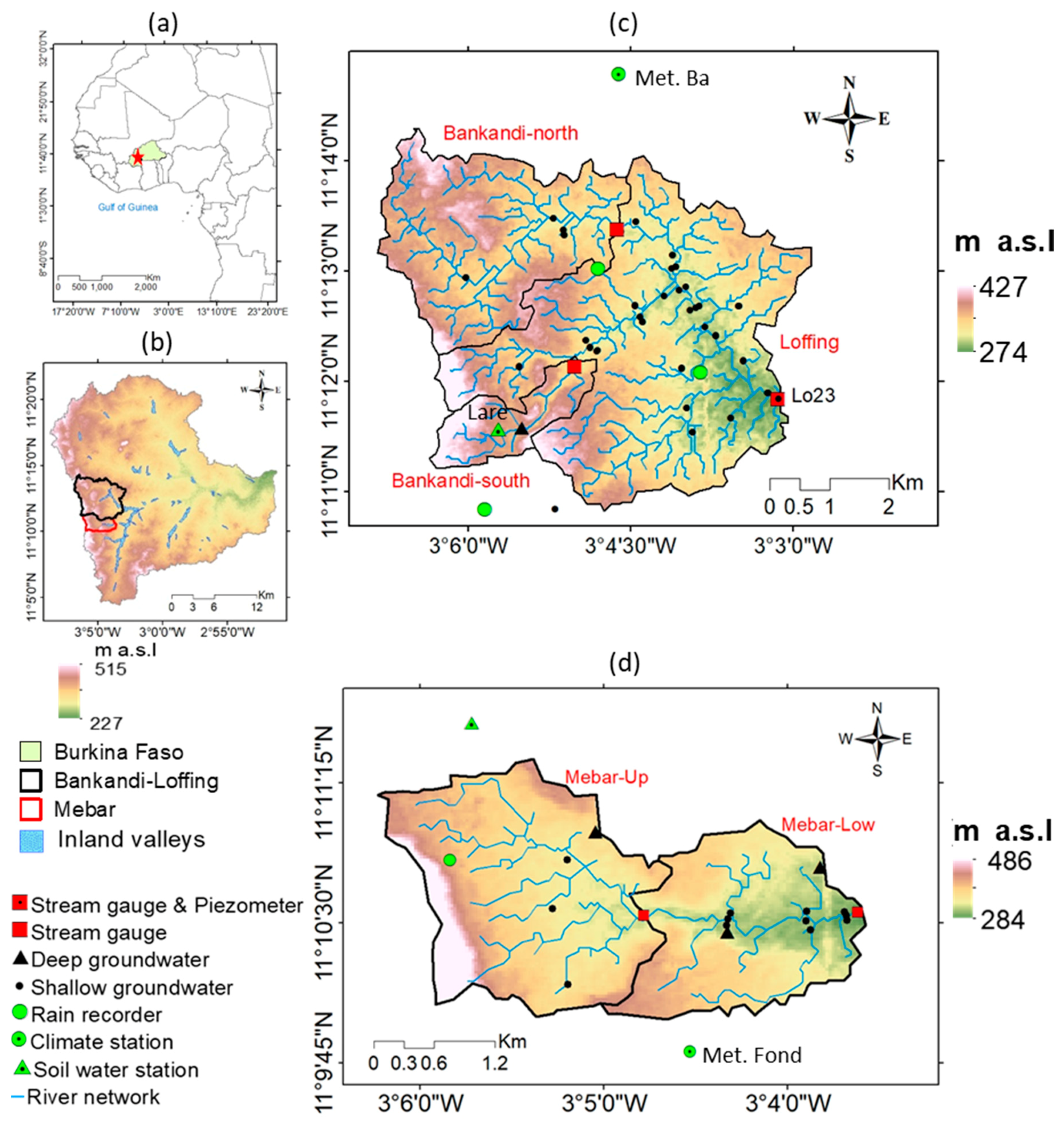
2.1. Study Area

The geomorphology of the catchments is characterized by flat landscapes. The mean slope is 4° in Bankandi-Loffing and 5° in Mebar. The most frequent slope is 3° in both investigated catchments and more than two thirds to three quarters of the catchments have a slope of 0° to 5°. This allows the formation of inland valleys that can easily be flooded during the rainy season.
The geology of Burkina Faso consists of Precambrian formations that are part of the West-African craton. The paleoproteozoic basement is made of Birimian green stone belts (2238 to 2170 million years old), volcano-sedimentary, and plutonic sequences [62]. The Ante-Birimian granites are found at the upstream areas and Birimian shists are located at the downstream areas of the investigated catchments [63]. The geology is made of crystalline rocks and the aquifer develops in faults, fractures, saprolites, and alluvial materials. The layers of saprolites are 10 to 30 m thick.
According to the soil classification of the World Reference Base [66], Plinthosols are the predominant soil types in the investigated area (Figure 2). They cover 50% of the Mebar catchment area and 73% of the Bankandi-Loffing catchment area. Cambisols and Gleysols are the second most observed soil types in the area. Cambisols and Gleysols account for 29% and 9% of the Mebar catchment, respectively, and each of the Cambisols and Gleysols represent 11% of the Bankandi-Loffing catchment. The texture of Plinthosols varies with soil depth from loam to clay whereas for Gleysols and Cambisols, the texture changes from clay loam or silt loam to silt clay loam. Plinthosols are frequently observed in uplands of inland valleys while Gleysols and Cambisols are located in the valley bottoms.
The vegetation is mainly of savanna type (a mix of shrubs, trees, and herbs) in both of the catchments (Figure 3). The savanna covers 40% of the Bankandi-Loffing catchment and 41% of the Mebar catchment. The forest coverage is considerably higher in Bankandi-Loffing (20% of the catchment area) than in Mebar (7% of the catchment area). The most cultivated food crops are millet (Panicum miliaceum), sorghum (Sorghum bicolor), and maize (Zea mays). Millet and sorghum are cultivated in 19% of the Mebar catchment area and 11% of the Bankandi-Loffing catchment area. Approximately 8% to 10% of both catchment areas are used for maize cultivation. Rice (Oryza sativa or Oryza glaberrima) is mainly cultivated in the valley bottoms of the inland valleys and is grown in 4% of the Mebar catchment area and 3% of the Bankandi-Loffing catchment area. Cotton is the major cash crop and accounts for 11% of the Bankandi-Loffing catchment area and 9% the Mebar catchment area. Grasslands in Mebar (9% of the catchment area) and Bankandi-Loffing (5% of the catchment area) are used for cattle grazing.

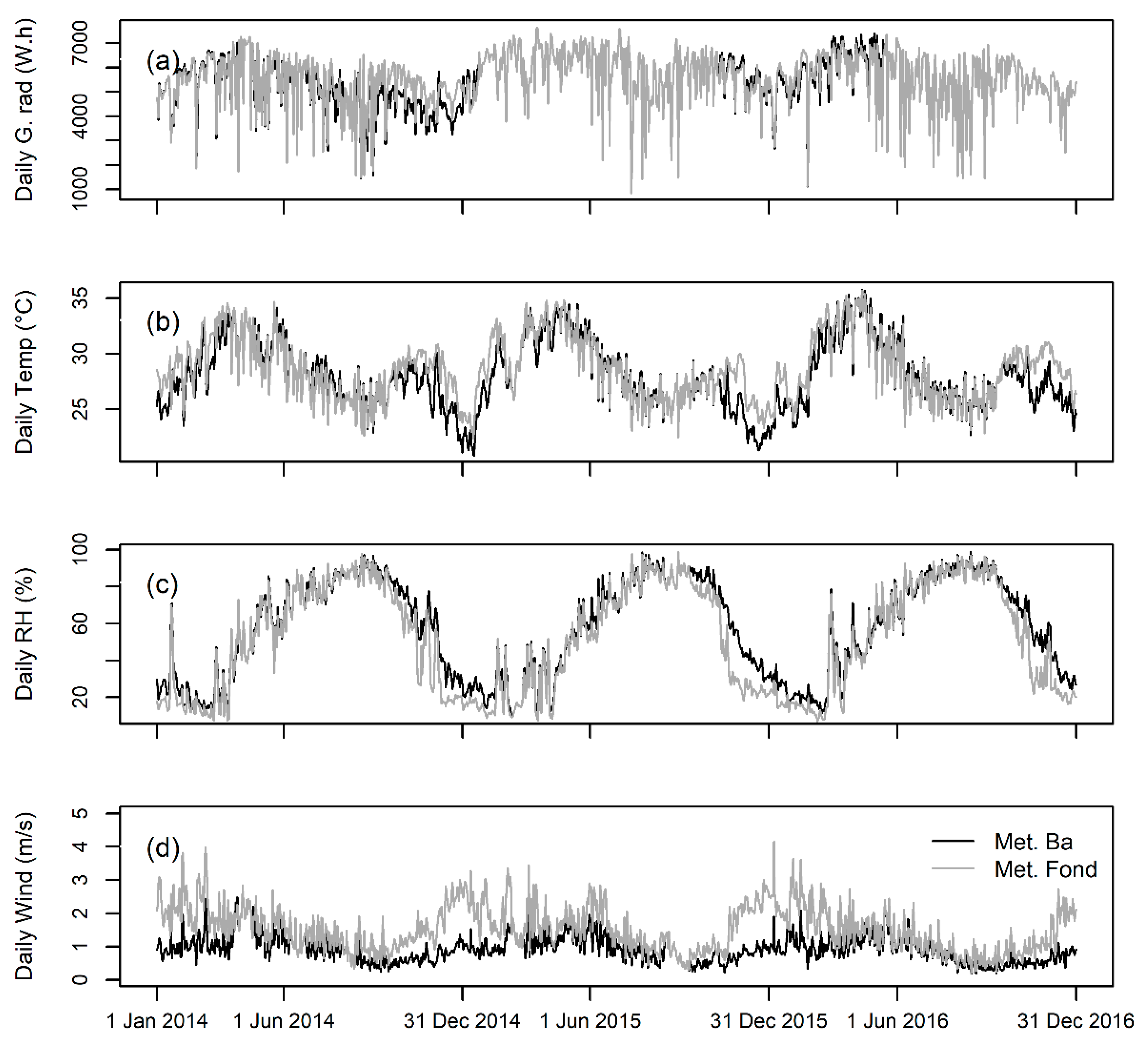
2.2. Observed Hydrological and Meteorological Data

While remote sensing climate data can be used for hydrological modeling at the mesoscale [59], at local scales such as the Bankandi-Loffing or Mebar catchments, this is hardly possible. The spatial resolution of remote sensing data products is too coarse for small scale studies as they range from 0.03° to 1° with an average resolution of 0.275° [69,70,71]. Therefore, in this study, an intensive instrumentation was undertaken in the investigated catchments. The installed and operated observation network consisted of five stream gauges, 43 piezometers in the shallow aquifer (depth < 5 m, with one of the piezometer (Lo23) equipped with a data logger), three rainfall recorders, two weather stations, and one soil moisture station (see Figure 1c,d for the spatial distribution of the instruments in the catchments).
Three-year time series data (2014–2016) were collected in both catchments. The temporal resolutions were 5 to 10 min for weather data (rainfall, air temperature, relative humidity, global radiation, and wind speed), 5 min for the discharge, 30 min for the soil water recording and the piezometer equipped with a data logger (Lo23), and weekly for manually measured piezometers and soil moisture.
The overview in Figure 4a–e shows that precipitation is concentrated in a unimodal rainy season (June to October). The daily precipitation exceeds 30 mm frequently. Therefore, the area is characterized by strong rainfall [10].
The streams in Figure 4f are ephemeral as most of them flow only during the rainy season. Base flow lasts longer in the Bankandi-Loffing (BaLof) and Mebar-low (Me-low) (Figure 1) stream stations compared to the other stations. This can be attributed to the contribution of the shallow aquifer to the flows in inland valleys.
The groundwater table as measured by the piezometer Lo23 shows a quick reaction to rainfall, which means that the shallow aquifer is replenished during the rainy season. In the dry season, groundwater level decreases steadily.
High temperature and wind speed as well as low humidity observed in the dry seasons (November to April) (Figure 5) characterize the Harmattan, which is the strong dry and hot wind that blows from the Sahara Desert through the study area during that period.
The slug test method after Bouwer and Rice [72,73] was used to estimate the hydraulic conductivity in 36 piezometers. The results (Table 1) were used in the parameterization of the hydrological model. It shows a large variability of Ks in the area (10−8 to × 10−5 m s−1). This large range may be explained by the variation of the geological formations that vary from alluvium in the valley bottoms to saprolites in the slope and uplands.
The valley bottoms tend to have alluvial materials on the top of saprolites. Therefore, the recharge of the weathered saprolite aquifer and the underlying migmatitic or granitic aquifer mainly depends on the hydraulic conductivity of the alluvial materials. This process is well described in a similar catchment in northern Benin [74]. The alluvium of the valley bottoms consists of sand or sandy loam and is permeable. Nevertheless, if they are made of silt or clay, their permeability is reduced.
The measured Ks was similar to the Ks of a fractured igneous and metamorphic rock [75]. However, caution is needed when using slug test data because they correspond to Ks at the vicinity of the investigated wells.

2.3. Methods

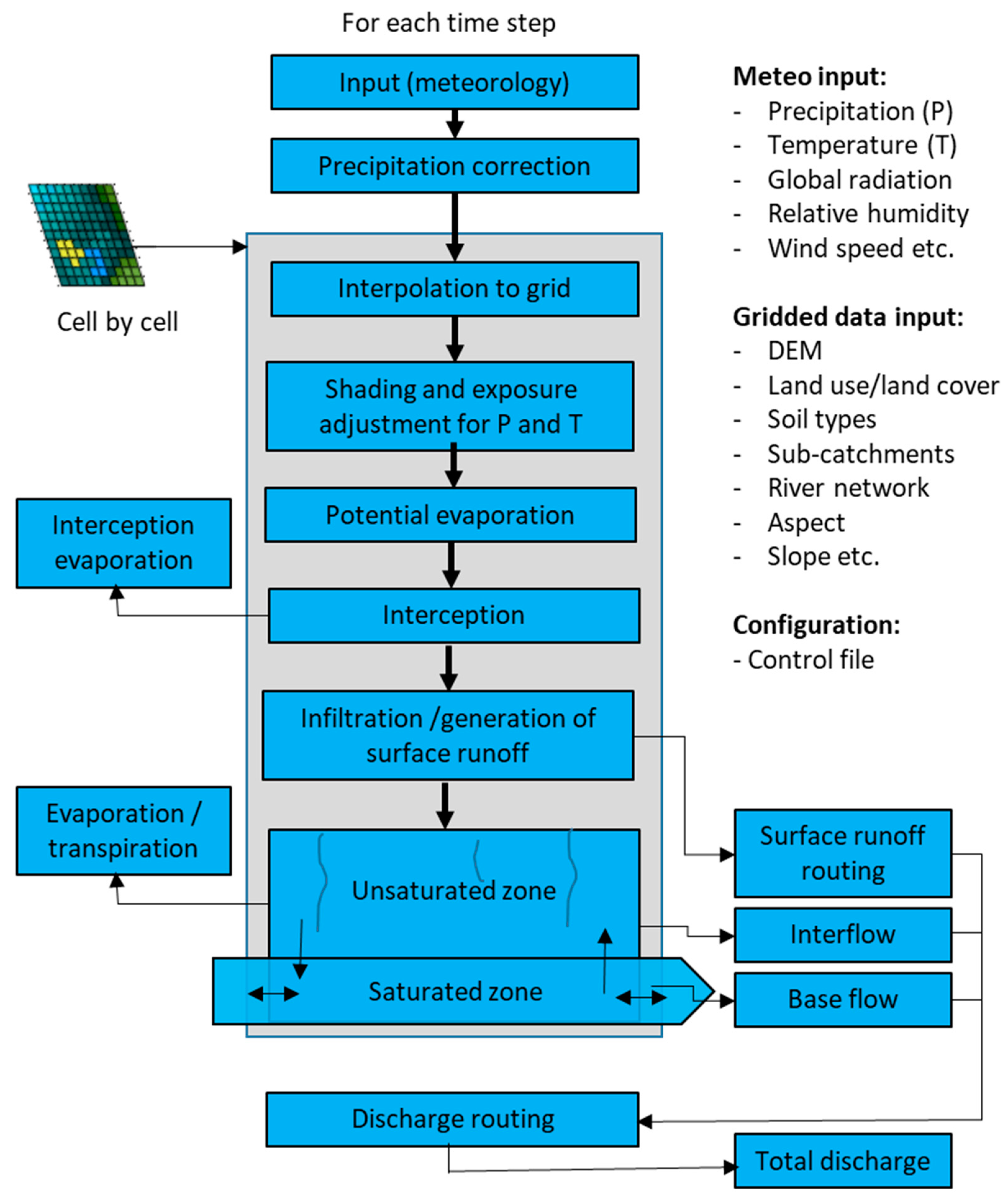
2.3.1. Hydrological Modeling

The Bankandi-Loffing and Mebar catchments were modeled using the grid-based, deterministic, and mainly physically-based hydrological model WaSiM (water flow and balance simulation model, version 9.10.01). Figure 6 is the schematic representation of WaSiM showing the hydrological processes applied in this study.
The input data include point meteorological data and gridded data. The point meteorological data were interpolated to gridded data using inverse distance weighting (IDW). The gridded input data include the land use/land cover (LULC) map at 5 m resolution [68] and the soil map at 90 m resolution [67]. The digital elevation model was based on the Shuttle Radar Topography Mission (SRTM) at 30 m resolution [64] using the topographic analysis program TANALYS [46]. These gridded data include catchment and sub-catchment delineations, stream network, slope, and aspect. The uniform grid-cell size of 30 m was applied for the discretization of the model.
Potential evapotranspiration was computed using the Penman–Monteith approach [76,77]. The evaporation from bare soil, open water bodies, and interception surfaces was computed separately from the transpiration from plants.
Actual evapotranspiration depends on the actual soil water content, capillary pressure, and LULC. It also considers the transpiration reduction due to oxygen or dryness stress [46,78].
Interception evaporation is conceptually modeled using a bucket approach and the interception parameters such as interception capacity (IntercepCap) and the leaf area index (LAI), which were defined for each of the four parameterized LULC types (croplands, savanna, settlements, and water bodies).
Infiltration into the unsaturated zone is physically modeled utilizing the Richards equation [47,79]. The van Genuchten equation [48] was employed for the numerical solution of the discrete form of the Richards equation. Sixteen numerical layers of various thicknesses were defined for each of the eleven parameterized soil categories (Figure 2). The total soil and shallow groundwater depth of 10 m was modeled.
Surface runoff is based on infiltration excess approach. Interflow is produced from a layer if the suction is equal or greater than a 3.45 m water column and the slope is significantly different from zero.
Base flow is computed conceptually using an exponential equation. Total discharge is the sum of surface runoff, interflow, and base flow. The Manning equation was utilized for discharge routing.
Groundwater table depth was determined by the relationship between the unsaturated zone model and groundwater model.
The model was calibrated for two years (2014–2015) and validated during 2016 at an hourly time step. A warmup period of six years was applied by repeating the climate variables of 2013 (rainfall, air temperature, air humidity, global radiation, and wind speed). This was necessary to stabilize the model and to obtain an initial model state close to the observed initial hydrological conditions.
Soil properties including saturated hydraulic conductivity (Ks), soil water at saturation (θs), residual soil water (θr), and van Genuchten parameters (n, α) were measured or computed using pedotransfer functions [80,81]. The LULC parameters such as root-depth, albedo, canopy surface resistance (rsc), evaporation surface resistance (rse), interception surface resistance (rsi), leaf area index (LAI), and vegetation cover fraction (VCF) were adapted from Yira et al. [81]. The parameterization in this study was based on Yira et al. because Bankandi-Loffing and Mebar are sub-catchments of their catchment.
The ranges of the optimized parameters (Table 2) were also adapted from Yira et al. [81]. The simulation environment for uncertainty and sensitivity analysis (SimLab 2.2; European Commission, [82]) software was utilized for the sampling and 200 parameter-sets were generated for each model. Latin Hypercube sampling was applied in order to ensure a fully stratified sampling of each parameter [83,84].

2.3.2. Model Performance Estimation

A multi-criteria approach was applied for model performance estimation in order to account for the deficiency of a single criterion approach [85]. The objective functions include the Nash–Sutcliffe Efficiency (NSE) [86], the Kling–Gupta Efficiency (KGE) [87,88], the coefficient of determination (R2) [89], and the percent bias (Pbias) [90].
NSE, KGE, R2, and Pbias were computed by Equations (1)–(4), respectively. Equation (4) was modified from Moriasi et al. [90].
N S E = 1 t = 1 n ( X s , t X o , t ) 2 t = 1 n ( X o , t μ o ) 2
K G E = 1 ( R 1 ) 2 + ( β 1 ) 2 + ( γ 1 ) 2 β = μ s μ o γ = C V s C V o = σ s / μ s σ o / μ o
R 2 = [ t = 1 n ( X s , t μ s ) ( X o , t μ o ) t = 1 n ( X s , t μ s ) 2 t = 1 n ( X o , t μ o ) 2 ] 2
P b i a s = t = 1 n ( X s , t X o , t ) t = 1 n ( X o , t ) 100
where n is the total number of time steps; Xs,t is the simulated discharge at a time t; Xo,t is the observed discharge at a time t; µs is the mean of the simulated discharges; µo is the mean of observed discharge; CVs is the coefficient of variation of the simulated discharge; CVo is the coefficient of variation of observed discharge; σs is the standard deviation of the simulated discharge; and σo is the standard deviation of the observed discharge.
The optimization of the model was oriented toward maximizing each of the first three objective functions (R2, NSE, and KGE) for discharge with a perfect model yielding in 1 for each of them. R2 ranged from 0 to 1, whereas NSE and KGE ranged from −∞ to 1. Concerning Pbias, the optimal value is zero and it ranges from −100% to +∞. The positive Pbias is equivalent to overestimation and the negative value is underestimation of the discharge by the model. A model was assessed as being satisfactory when NSE > 0.5 and −25% < Pbias < +25% [90]. A lower satisfactory limit of 0.5 was also considered for KGE.
The most optimal parameter-set is assumed to be the one with the highest KGE for discharge. This is due to the fact that KGE not only incorporates R2 in its equation, but also accounts for both conditional and unconditional biases [87,91]. According to Equation (2), maximizing each of the components of KGE will result in maximizing KGE [88].
R2 was not chosen to select the optimal simulation as it is susceptible for systematic errors. The use of only R2 for model performance estimation might be misleading [85].
Although NSE is the most employed dimensionless objective function in hydrological modeling, it has been criticized for using mean observed discharge as the baseline. This might lead to overestimation of model performance when a significant seasonal variation of runoff is observed [87].

2.4. Spatial Transposability of the Hydrological Model

The robustness of the hydrological model was estimated by investigating its spatial transposability of the hydrological model from Bankandi-Loffing to Mebar. The Bankandi-Loffing catchment was first calibrated and validated. The resulting parameter-set that gives the best simulation for discharge was then transferred to the Mebar catchment without recalibration. Therefore, the land use table for land use/land cover parameters and the soil table for soil parameters in WaSiM were not changed. In total, four land use/land cover classes and eleven soil types were modeled. The robustness of the hydrological model was evaluated by quantifying the Mebar model performance for discharge using the numerical indicators (R2, NSE, KGE, Pbias) and the graphical method.

3. Results and Discussion

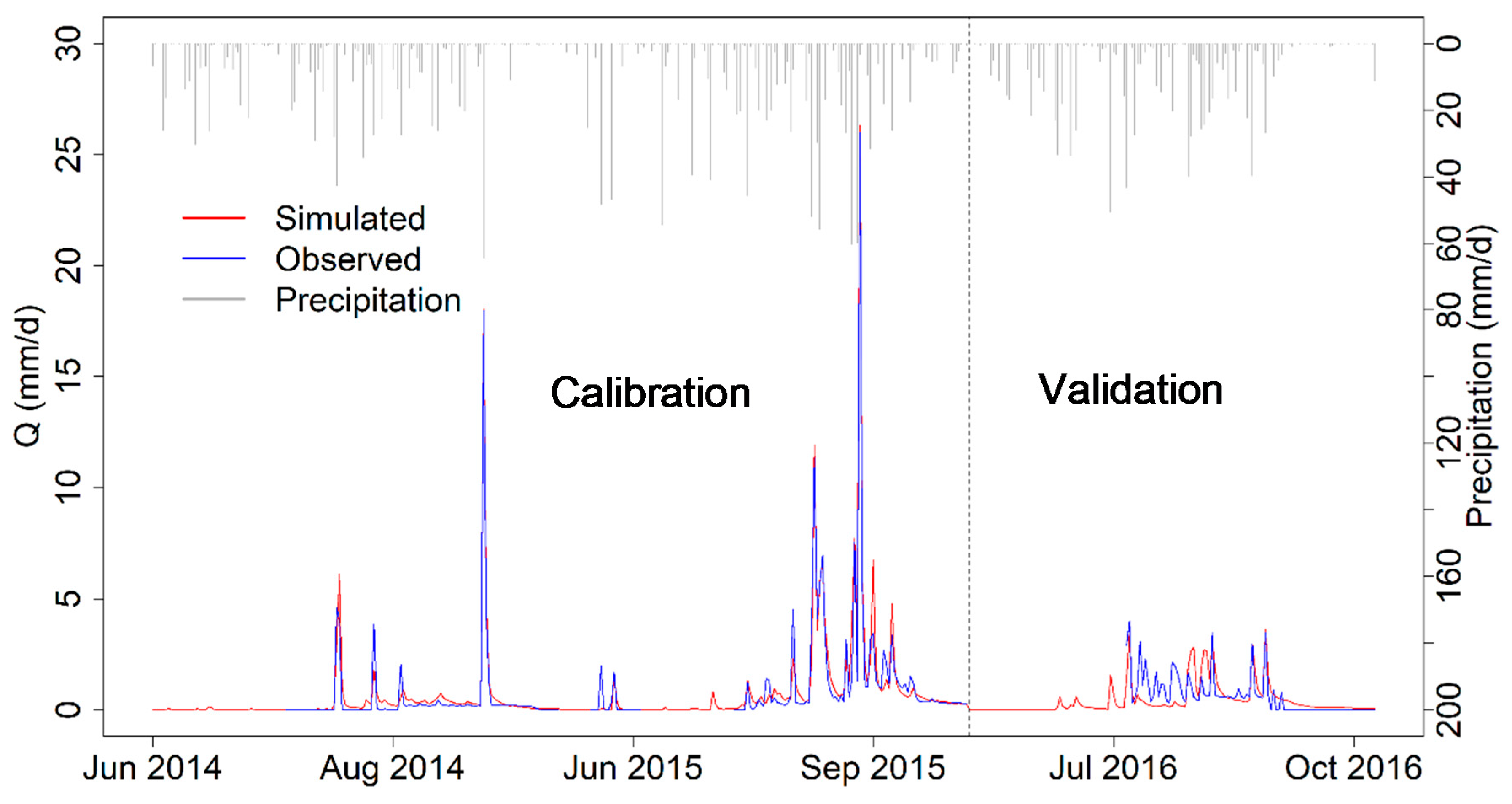
3.1. Calibration and Validation of the Bankandi-Loffing Model

3.1.1. Model Performance

WaSiM performed very well, as shown by the objective functions (Table 3). NSE, KGE, and R2 were larger than 0.5 in most cases in the calibration and the validation periods. In general, the model performed as well in the upstream area (Bankandi-north) as in the overall catchment (Bankandi-Loffing). R2 ranged from 0.47 to 0.95, NSE from 0.40 to 0.95, and KGE from 0.57 to 0.84 at the outlet and at the Bankandi-north stream station and for the calibration and validation periods. The slight decrease in the model performance might be attributed to overcalibration as the best simulation was selected based on the highest value of the objective functions [56]. Pbias ranged between 1.6 and 29.4%, indicating a slight overestimation of the discharge by the model.
In addition to the assessed numerical model performance, the visual performance of the model, which is illustrated by the hydrographs in Figure 7 and Figure 8, revealed very good results for the upstream area and the overall catchment. Temporal dynamics as well as most of the high and low flows were well simulated in the calibration and validation periods. However, as already shown previously in the numerical performance analyses, the model performed better in the calibration period when compared to the validation period, especially at the Bankandi-north station. Some peaks were not well captured by the model at that station. This is partly due to the quality of the observed discharge data as a sensor dysfunction was noted in the period.
The comparison of the spatial mean simulated soil moisture and observed top soil (10 cm depth) moisture at Lare (Figure 1c) during 2014 showed good agreement (Figure 9). It should be noted that the model was not calibrated for soil moisture as most of the soil parameters were measured in the field or laboratory. Each of the calculated objective functions (R2, NSE, and KGE) were higher than 0.5. The graphical comparison showed good agreement between the simulated and observed soil moisture and the model simulated the initial soil moisture well. This indicates that the applied six-year warmup period is sufficient to stabilize the model. Although some discrepancies can be observed in the rainy season and the dry season, the temporal dynamics were well captured overall. Good top soil modeling is important for runoff generation and partitioning between different soil layers and the aquifer.
In addition to the soil moisture, the model was validated by comparing the average simulated monthly groundwater level at the outlet sub-catchment (Loffing) with the observed groundwater level at the piezometer Lo23 located at the outlet of the catchment (Figure 1c). The comparison was done after subtracting the elevation difference between the piezometer and the Loffing sub-catchment from the areal simulated groundwater level. Figure 10 suggests a short delay of some simulated groundwater level peaks compared to the observed peaks. This leads to unsatisfactory results with regard to R2 and NSE. However, in general, the temporal dynamics and the amplitudes of variations are acceptable with a KGE of 0.5.

3.1.2. Water Balance

A considerable inter-annual variation of rainfall was observed during the three year period of monitoring (Table 4). The difference in annual rainfall between the years 2014 and 2015 was 223 mm (21% of the mean annual rainfall).
The actual evapotranspiration (ETa) represented 45% of the potential evapotranspiration (ETp). This indicates a water limited and not an energy limited catchment. During the dry years (2014 and 2016), decreases of soil water storage were observed whereas in the wet year of 2015, an increase in soil water storage was noted. This is indicated by a negative change in storage (delta S) in the former years and positive delta S in the latter year (Table 4). The succession of dry and wet years resulted in a more or less stable system from 2014 to 2016 with a relatively low annual mean delta S for the overall Bankandi-Loffing catchment (delta S = −12 mm). This means that water stored in the soil and aquifers during the wetter years is lost through evapotranspiration and groundwater flow during the dry years. Therefore, consecutive dry years similar to that in 2014 will not only jeopardize the livelihoods of the majority of the farmers who practice rainfed agriculture, but will also affect the general hydrological processes and water resources.
At the catchment scale of Bankandi-Loffing, the evaporation was five times as high as the transpiration. This can be explained by the long dry season of seven to eight months per year, in which most farmers cease activities, the herbaceous vegetation dries out completely, and most of the trees lose their leaves in savanna areas. This leads to a significant reduction of transpiration by plants. However, a relatively higher coverage of permanent plants (forest) in the Bankandi-north sub-catchment compared to the Bankandi-south and the Loffing sub-catchments can partially explain the significant difference of transpiration between the former and the latter sub-catchments.
The observed variability in annual rainfall led to a more pronounced variation of the observed runoff volume. For instance, the variation of rainfall from 2014 to 2015 was 21% of the mean annual rainfall, but the increase in total runoff was approximately four times the increase in rainfall (approximately 88% of the mean runoff). The overall coefficient of variation of total runoff was 36% of the mean annual runoff during the observation period (2014–2016). The mean total runoff coefficient at the outlet was 14% of the mean annual rainfall, but there was a significant contrast between upstream sub-catchments (Bankandi-south and Bankandi-north) and the downstream sub-catchments (Loffing). The highest runoff coefficient was obtained at the downstream sub-catchment due to a high contribution of base flow to streamflow. The high contribution of base flow can be explained by the shallowness of the groundwater table at this sub-catchment compared to the upland sub-catchments.
Table 4 also indicates that interflow is the main runoff component in the Bankandi-south sub-catchment and represents 60% of the total runoff. It is noteworthy that interflow decreases from the upstream sub-catchments to the downstream. Yira et al. [81] obtained 56% on average between 2011 and 2014 and 59% in 2014 while modeling a 6.5 times larger catchment than Bankandi-Loffing. In a similar catchment in northern Benin simulated for the period 1998–2004 by Cornelissen et al. [92], the interflow was 65% of the total runoff using the UHP-HRU model and 38% using WaSiM. Based on field experiments, the authors conclude that UHP-HRU has a better representation of the hydrological dynamics of the catchment. Moreover, in the Volta basin, Kasei [49] found 68% interflow at the northern area and 60% at the southern area where the Dano catchment is located. However, interflow is not the dominant runoff component in the other Bankandi-Loffing sub-catchments. For instance, in Bankandi-north, surface flow is the most dominating component of runoff (44% of total runoff) and in the Loffing sub-catchment and the overall Bankandi-Loffing catchment, base flow largely dominates streamflow (57% and 45% of total runoff, respectively). An increase of base flow was noted from the upstream to downstream section. The comparison between observed base flow [93] was estimated using analytical hydrograph decomposition and the simulated base flow showed close similarities. For instance, the observed base flow at Bankandi-south, Bankandi-north, and Bankandi-Loffing represented 9%, 16%, and 42% of the total runoff, respectively, and the simulated base flow was 7%, 17%, and 45% for the respective sub-catchments. The difference between these findings and the previously cited studies is due to the fact that a considerable part of the downstream area of the investigated catchment is occupied by valley bottoms of inland valleys. The proximity of the aquifer level to the ground surface allows for a significant contribution of base flow in valley bottoms.
It is also important to recall that the partitioning of runoff into its components is not only influenced by rainfall intensity and physical properties of soil and slope, but also by the hydrological conditions of the catchment before flood events [94]. Furthermore, macropore density and distribution drive runoff component generation in the West African savanna. For instance, Giertz et al. [95] reported 219 bio-pores per m2 in a savanna plot of a catchment in northern Benin, whereas only 60 bio-pores were counted in the cultivated field. With the conversion of savanna to croplands in the Dano catchment [81,96], the current pattern of runoff components is likely to change in favor of surface flow. This might lead to significant soil fertility loss due to high soil erosion [97]. Therefore, an improvement of the current traditional water and soil management should be planned.

3.2. Transfer of Bankandi-Loffing Parameters to the Mebar Model without Recalibration

The parameter-set that gave the highest KGE during calibration and validation of the Bankandi-Loffing model was directly applied to the Mebar model without recalibration and the calculated model performance (Table 5) showed very good results during the years 2014–2015. The Mebar model performed even better than Bankandi-Loffing during the period 2014–2015. R2, NSE, and KGE were approximately 0.3 point higher in Mebar than in Bankandi-Loffing.
However, in 2016, the Mebar model resulted in a R2 and NSE lower than the Bankandi-Loffing model, but the values of the objective functions remained higher or equal to 0.6. In contrast to R2 and NSE, the Pbias was significantly improved in the Mebar model (12%) compared to Bankandi-Loffing (29%) in 2016. Regarding KGE, the performance difference between the non-recalibrated Mebar model (KGE 0.59) and the Bankandi-Loffing model (KGE 0.57) was negligible during 2016.
Moreover, while the hydrograph (Figure 11) shows that the non-recalibrated Mebar model had fallen slightly short in matching some peaks, the performance was good in general.
The numerical and graphical Mebar model performances showed good results in both periods of 2014–2015 and 2016. Therefore, the transfer of the parameters from the Bankandi-Loffing model to Mebar can be assessed as a success. However, it is important to note that the calibration and validation period of the initial Bankandi-Loffing model and the transfer period for Mebar were identical (2014–2016). The period is characterized by two dry years separated by a wet year. These findings therefore need to be tested for longer time periods and in different climate conditions in order to fully evaluate the robustness of the model in transferring parameters from one catchment to another.

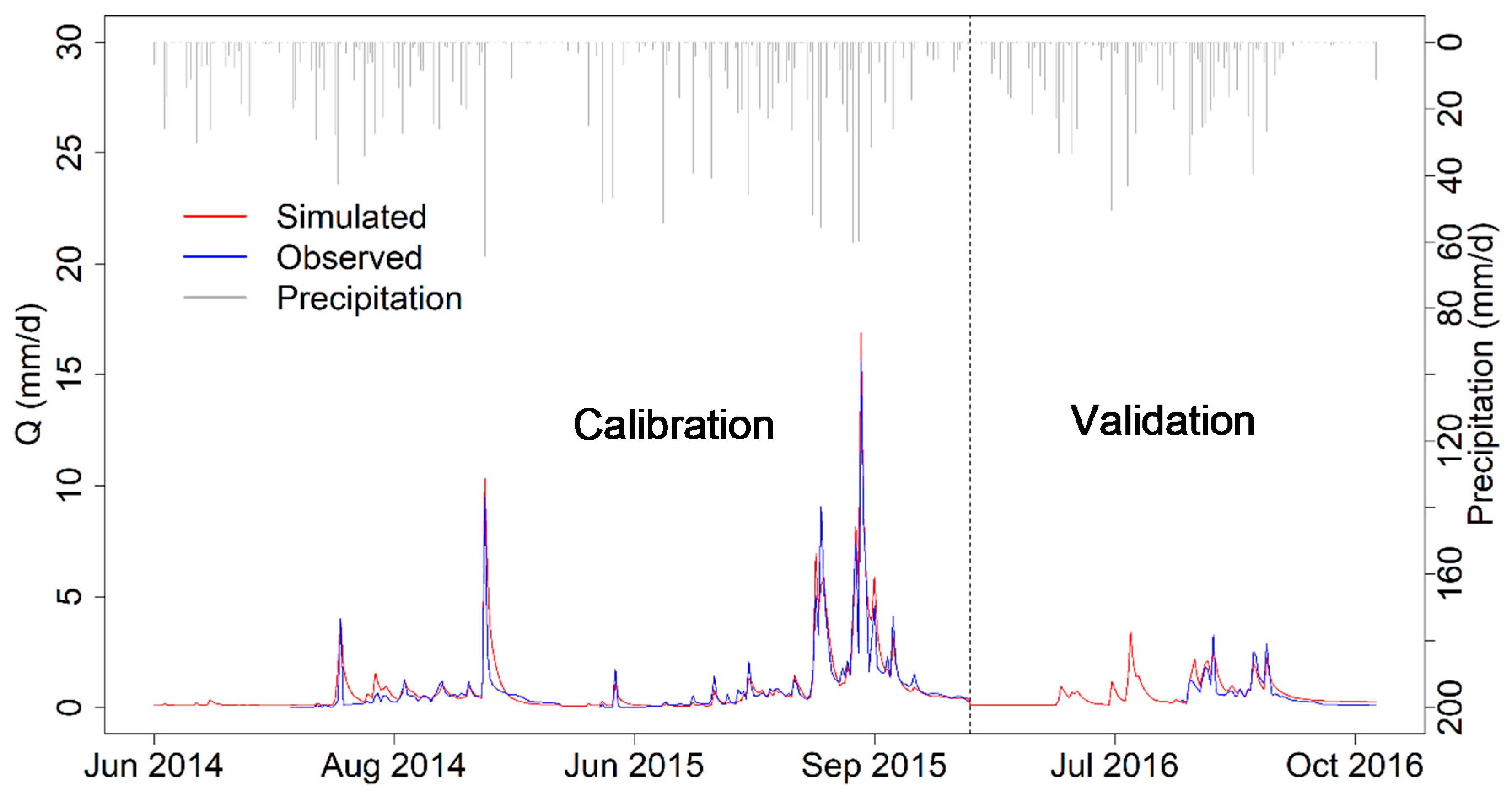
3.3. Recalibration and Validation of the Mebar Model

The Mebar model was calibrated for 2014–2015 and validated for 2016 in order to establish a reference Mebar model for evaluating the quality of the parameter transfer. The summary (Table 6) indicates an improvement in model performance with the recalibration. Each objective function (R2, NSE, and KGE) was greater than 0.9 in the calibration period and 0.7 in the validation year. The increase of R2 and NSE (0.02 in calibration period and 0.06 in validation period) with the recalibration was lower than the increase of KGE (0.11 in calibration and 0.12 in validation periods) during both the calibration and the validation periods. This may be explained by the combined effect of the increase in R2 and NSE. KGE is a function of the correlation coefficient, which in itself is the square root of R2, the bias ratio, and the variability ratio, which can be estimated in NSE [88].
The comparison of the simulated hydrograph and measured hydrograph (Figure 12) showed a good agreement between the hydrographs and was consistent with the numeric model performance assessment.
The water balance of the best simulation of the Mebar model (Table 7) revealed many similarities with Bankandi-Loffing. The actual evapotranspiration (ETa) was 85% of rainfall, physical evaporation accounts for 79% of ETa, and only 45% of the potential evapotranspiration (ETp) could actually evaporate in the form of ETa given the water limited conditions of the area.
In contrast to Bankandi-Loffing, instead of base flow, interflow is the main component of runoff in Mebar (39% of total runoff), followed by surface flow (32% of total runoff). The contrast between Mebar and Bankandi-Loffing can be partly explained by the difference in slopes and land use. A large area of the Mebar catchment is located between the Ioba Mountains and is mostly covered by uplands while the Bankandi-Loffing catchment is characterized by flat land and valley bottoms of the inland valleys. The estimated mean slope is 5.1% with a standard deviation of 4.6% in the Mebar catchment, whereas the mean slope is 4.1% with a standard deviation of 3.1% in the Bankandi-Loffing catchment. Concerning land use, croplands occupy a larger area in Mebar (42%) than in Bankandi-Loffing (33%). The slope and land use may be responsible for the higher contribution of both surface runoff and interflow in Mebar compared to Bankandi-Loffing.

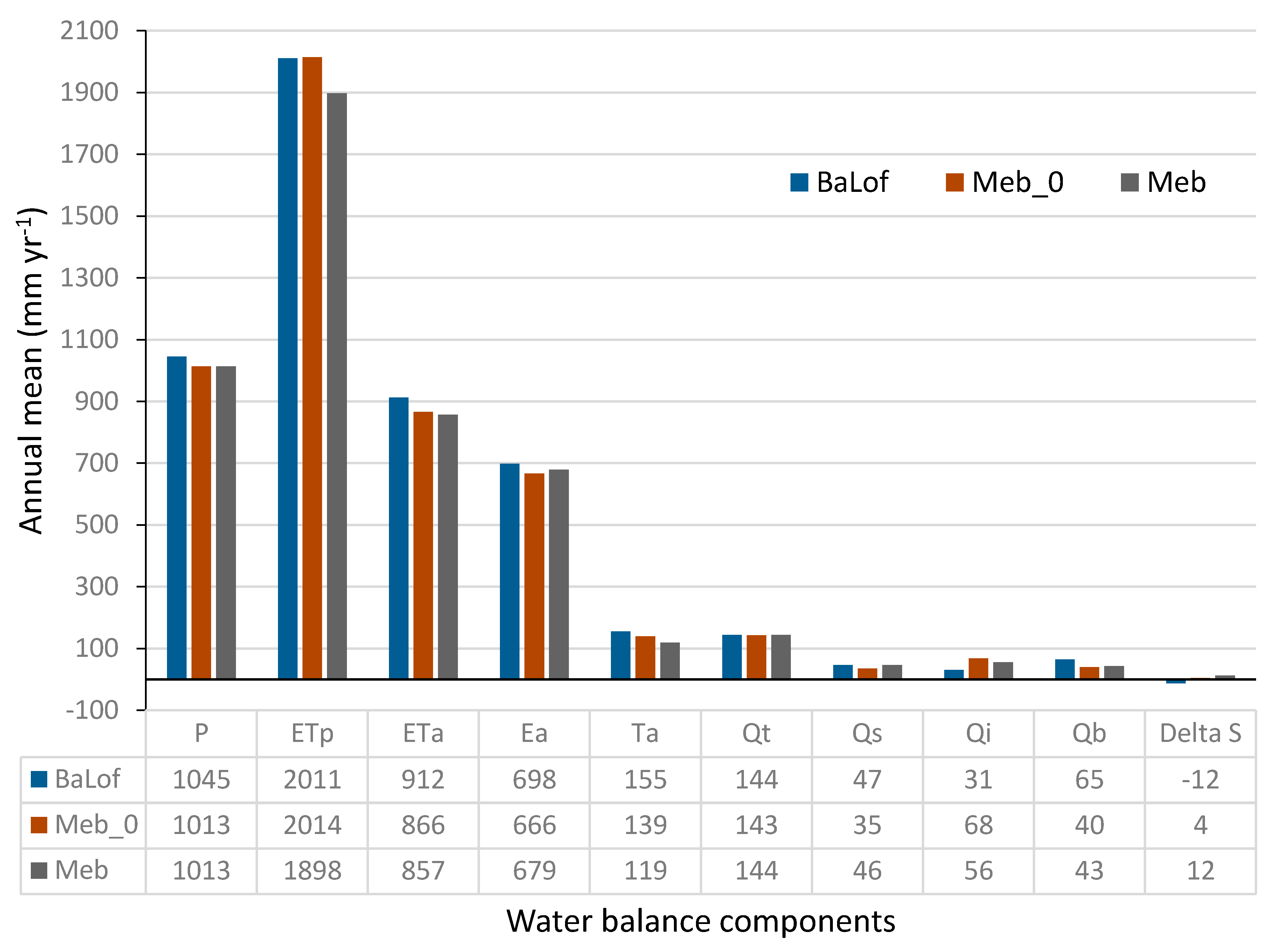
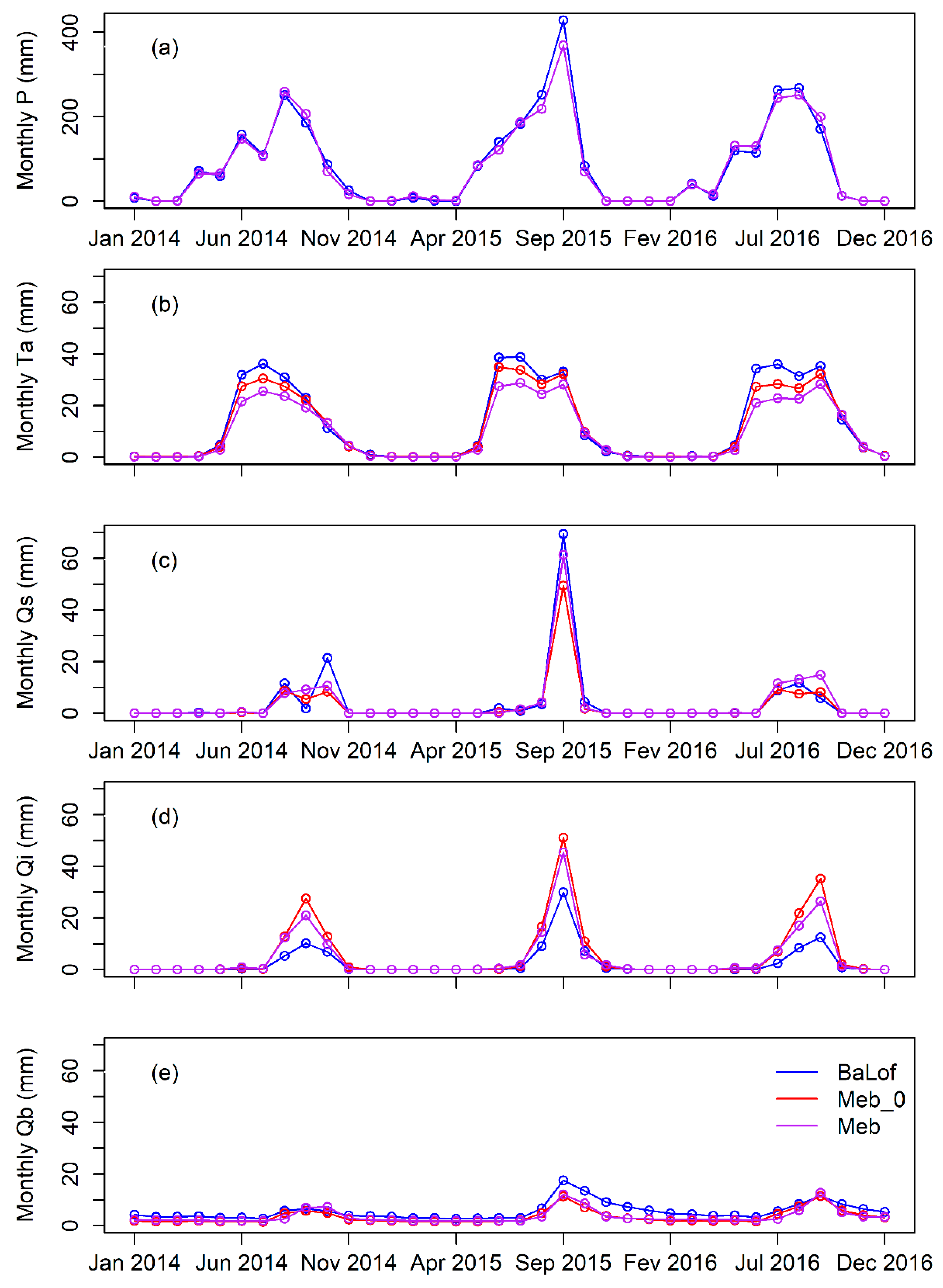
3.4. Comparing Water Balance between Bankandi-Loffing and Mebar

The comparison of the mean annual water balance for Bankandi-Loffing (BaLof), Mebar before (Meb_0), and after (Meb) recalibration (Figure 13) showed only 3% lower rainfall in Mebar models (Meb_0 and Meb) compared to Bankandi-Loffing and no rainfall rate difference between Meb_0 and Meb was noted. This could in part explain the similar simulated total runoff for the three models. However, significant differences were noted between the simulated runoff components for the three models and the variations of runoff components between the models did not indicate any trend.
Furthermore, the potential evapotranspiration (ETp) did not seem to continuously decrease between the models, but the total actual evapotranspiration (ETa) and the actual transpiration (Ta) did. If only Meb_0 and Meb are examined, it becomes clear that the recalibration led to reductions in ETp, ETa, and Ta, while actual evaporation (Ea) increased. This behavior seems to be caused by the increase of the mean canopy surface resistance (rsc) from 64 to 73 s m−1 and the evaporation surface resistance (rse) increased from 50 to 52 s m−1 due to land use land cover differences.
Figure 14 presents monthly temporal variations of the water balance components. For very intense rainfall conditions such as the conditions in September 2015, the peak of surface runoff was higher than the interflow. Conversely, under moderate rainfall conditions like in September 2014 and September 2016, the peak of surface runoff was lower than the interflow. However, the peaks of the base flow stayed lower than the surface runoff and interflow, but were sustained for a longer time compared to the surface runoff and interflow. As for the transpiration, their rates were only considerable during the rainy seasons (June to October). This is consistent with the field observations, which present much reduced plant activities in dry seasons due to water unavailability. The herbaceous vegetation completely dies out and most trees lose their leaves, therefore, most of their ability to transpire.

3.5. Transferred Model Parameter Values

Table 8 presents the final parameter values for land use/land cover and soil after calibration and validation of the Bankandi-Loffing model and which were transferred to Mebar. Some parameters such as the thresholds for oxygen stress (TReduWet) and hydraulic head for starting dryness stress (HReduDry) both used for calculating transpiration were constant and were not optimized in this study. Oxygen stress was set to 5% of fillable porosity and the parameter HReduDry was set to 3.45 m of water column, which is approximately the soil suction at the field capacity [47,98,99].
Minimum values for the parameters canopy surface resistance (rsc), evaporation surface resistance (rse), albedo, leaf area index (LAI), vegetation cover fraction (VCF), specific thickness of the water layer on the leaves (IntercpCap), and aerodynamic roughness length (Z0) were set for open water bodies. This ensures the maximum evaporation rate from the open water bodies. The root depth in savanna is deeper than in the other land use classes as savanna has higher tree and shrub density compared to croplands and settlements. In general, the land use parameters selected in this study are realistic because the estimated potential evapotranspiration was in the acceptable range of the region [81,92,100,101,102].
The range of saturated hydraulic conductivity (Ks) was based on field measurements. For the first two soil horizons, soil analysis and pedotransfer functions, which estimated soil hydrological properties from soil texture and bulk density, were applied while for the third horizon, results from the slug test results were used. The Ks values corresponded to loam, clay loam, or silt clay loam texture, which is in line with previous studies in the region [50,93,95]. The saturated soil moisture (θs), the residual soil moisture (θr), and the van Genuchten empirical parameters (α, n) were estimated using a soil survey data and pedotransfer functions [50].
Effective parameters cannot be measured, therefore, the values of sensitivity analysis were used in this study [81,103]. That is, the case of drainage density (dr), storage coefficient for surface runoff (kd), storage coefficient for interflow (kh), storage coefficient for base flow (kb), and scaling factor for base flow (q0). Given that the effective parameters have no physical meaning, their reasonableness is indirectly judged on the basis on the quality of the simulations.

4. Conclusions

This study successfully tested the robustness of the hydrological model WaSiM in two data sparse small-scale catchments of Burkina Faso. It is one of the rare studies in West Africa where the multivariate model performance approach is coupled with the spatial transposability of a hydrological model to evaluate the robustness of the predictions.
This has been possible because of an intensive instrumentation of the two ungauged catchments. Two weather stations recording rainfall, air temperature, global radiation, relative humidity, and wind speed were installed and operated during the three-year field investigation period. To account for high spatial rainfall variability, three additional rain recorders were uniformly installed in the catchments. Five stream gauges, 43 piezometers, and one soil station were part of our instrumentation. High spatial and temporal resolutions of hydrological, meteorological, and spatially distributed data (soil, LULC, topography, etc.) were collected.
The collected data allowed us to successfully parameterize, calibrate, and validate the physically-based hydrological model WaSiM for the Bankandi-Loffing catchment. The four applied objective functions (R2, NSE, KGE, and Pbias) suggest that WaSiM performed well in modeling the discharge of the small-scale inland valley catchment. R2, NSE, and KGE ranged from 0.6 to 0.9, and Pbias was lower than 30% during the calibration (2014–2015) and validation (2016) periods.
In addition to the discharge, the model performance was assessed for soil moisture and groundwater table depth. The result suggests that the multivariate model performance assessment was successful. Soil moisture and groundwater table depth were in general well modeled and the initial soil moisture conditions were well reproduced by the model.
The robustness of the model was evaluated by investigating the spatial transposability of the hydrological model from the Bankandi-Loffing to Mebar model. The best parameter-set resulting from the calibration and validation of Bankandi-Loffing was transferred to Mebar without any recalibration of the Mebar model. The results clearly show a very good performance of WaSiM. Therefore, the parameter-set achieved in this study can be useful for ungauged inland valley small-scale catchments in the region. However, considering that this investigation occurred for the same period and that the investigated period was relatively short, the robustness of the model should be tested for longer periods in different climates and catchment conditions.
The analysis of the water balance indicates that evapotranspiration is quantitatively the most important hydrological process in the area and that physical evaporation largely dominates evapotranspiration. The average annual loss of 688 mm (approximately 67% of annual rainfall) is due to the fact that evaporation does not contribute to biomass production. Therefore, evaporation reduction techniques such as agroforestry or mulching can be implemented as part of the effort for better management of soil and scarce water resources. Moreover, 14% of annual rainfall runs out of the catchment as total discharge without being used. Therefore, soil water management techniques could be set up in order to slow down the surface flow and thereby increase the infiltration and soil water availability, while keeping the impact on downstream in an acceptable range. The success of the implementation of the water resource management depends on the level of involvement of stakeholders.
Interflow dominates runoff in the Mebar catchment and upstream area of Bankandi-Loffing whereas base flow is the major runoff component in the downstream area of Bankandi-Loffing, which has a large area of inland valley bottoms. Due to the trend of conversion of savanna into croplands as a result of population growth, surface flow will presumably increase, leading to an increase in soil erosion. Consequently, adaptation strategies should be planned accordingly. Supplementing the current erosion technique (stone-belt) with agroforestry and/or mulching might be considered.

Author Contributions

M.I., B.D., B.T., B.I., Y.Y., G.S. and T.P. designed the study, developed the methodology, and wrote the manuscript. M.I., B.T., B.I., and G.S. performed the field work and collected the data. M.I., B.D., Y.Y. and T.P. conducted the computer analysis. All authors have read and agreed to the published version of the manuscript.

Funding

This research was funded by the German Federal Ministry of Education and Research (BMBF) under the project West African Science Service Center on Climate Change and Adapted Land Use (WASCAL), grant number 01LG1202A, and by the Islamic Development Bank through the Merit scholarship program, grant number 600029612.

Conflicts of Interest

The authors declare no conflicts of interest. The funders had no role in the design of the study; in the collection, analyses, or interpretation of data; in the writing of the manuscript, or in the decision to publish the results.

References

  1. Denis, S.; Gapia, M.; Pokam, W.; Losembe, F.; Mfochivé, O. The Link between Forest, Water and People: An Agenda to Promote in the Context of Climate Change in Central Africa. In Nature and Faune: Managing Africa’s Water Resources: Integrating Sustainable Use of Land, Forest and Fisheries; Bojang, F., Ndeso-Atanga, A., Eds.; FAO: Accra, Ghana, 2012; pp. 48–51. Available online: http://www.fao.org/africa/publications/nature-and-faune-magazine/ (accessed on 3 June 2019).
  2. Schmengler, A.C. Modeling Soil Erosion and Reservoir Sedimentation at Hillslope and Catchment Scale in Semi-Arid Burkina Faso. Ph.D. Thesis, University of Bonn, Bonn, Germany, 2011. Available online: http://hss.ulb.uni-bonn.de/diss_online elektronisch publiziert (accessed on 17 October 2019).
  3. Braman, L.M.; Van Aalst, M.K.; Mason, S.J.; Suarez, P.; Ait-Chellouche, Y.; Tall, A. Climate Forecasts in Disaster Management: Red Cross Flood Operations in West Africa, 2008. Disaster 2013, 37, 144–164. [Google Scholar] [CrossRef] [Green Version]
  4. Cornforth, R. Overview of the West African. Weather 2011, 67, 59–65. [Google Scholar] [CrossRef] [Green Version]
  5. Lebel, T.; Ali, A. Recent Trends in the Central and Western Sahel Rainfall Regime (1990–2007). J. Hydrol. 2009, 375, 52–64. [Google Scholar] [CrossRef]
  6. Mougin, E.; Hiernaux, P.; Kergoat, L.; Grippa, M.; De Rosnay, P.; Timouk, F.; Le Dantec, V.; Demarez, V.; Lavenu, F.; Arjounin, M. The AMMA-CATCH Gourma Observatory Site in Mali: Relating Climatic Variations to Changes in Vegetation, Surface Hydrology, Fluxes and Natural Resources. J. Hydrol. 2009, 375, 14–33. [Google Scholar] [CrossRef] [Green Version]
  7. Niang, I.; Ruppel, O.C.; Abdrabo, M.A.; Essel, A.; Lennard, C.; Padgham, J.; Urquhart, P. Africa. In Climate Change 2014: Impacts, Adaptation and Vulnerability-Contributions of the Working Group II to the Fifth Assessment Report of the Intergovernmental Panel on Climate Change; Barros, V.R., Field, C.B., Dokken, D.J., Mastrandrea, M.D., Mach, K.J., Bilir, T.E., Matterjee, M., Ebi, K.L., Estrada, Y.O., Genova, R.C., et al., Eds.; Cambridge University Press: Cambridge, UK; New York, NY, USA, 2014; pp. 1199–1265. [Google Scholar] [CrossRef]
  8. Nka, B.N.; Oudin, L.; Karambiri, H.; Paturel, J.E.; Ribstein, P. Trends in Floods in West Africa: Analysis Based on 11 Catchments in the Region. Hydrol. Earth Syst. Sci. 2015, 19, 4707–4719. [Google Scholar] [CrossRef] [Green Version]
  9. Oguntunde, P.G.; Abiodun, B.J.; Lischeid, G. Impacts of Climate Change on Hydro-Meteorological Drought over the Volta Basin, West Africa. Glob. Planet. Chang. 2017, 155, 121–132. [Google Scholar] [CrossRef]
  10. Salih, A.A.M.; Elagib, N.A.; Tjernström, M.; Zhang, Q. Characterization of the Sahelian-Sudan Rainfall Based on Observations and Regional Climate Models. Atmos. Res. 2018, 202, 205–218. [Google Scholar] [CrossRef]
  11. Tschakert, P.; Sagoe, R.; Ofori-Darko, G.; Codjoe, S.N. Floods in the Sahel: An Analysis of Anomalies, Memory, and Anticipatory Learning. Clim. Chang. 2010, 103, 471–502. [Google Scholar] [CrossRef]
  12. Descroix, L.; Mahé, G.; Lebel, T.; Favreau, G.; Galle, S.; Gautier, E.; Olivry, J.-C.; Albergel, J.; Amogu, O.; Cappelaere, B. Spatio-Temporal Variability of Hydrological Regimes around the Boundaries between Sahelian and Sudanian Areas of West Africa: A Synthesis. J. Hydrol. 2009, 375, 90–102. [Google Scholar] [CrossRef]
  13. Di Baldassarre, G.; Montanari, A.; Lins, H.; Koutsoyiannis, D.; Brandimarte, L.; Blschl, G. Flood Fatalities in Africa: From Diagnosis to Mitigation. Geophys. Res. Lett. 2010, 37, 2–6. [Google Scholar] [CrossRef] [Green Version]
  14. Frappart, F.; Hiernaux, P.; Guichard, F.; Mougin, E.; Kergoat, L.; Arjounin, M.; Lavenu, F.; Koité, M.; Paturel, J.-E.; Lebel, T. Rainfall Regime across the Sahel Band in the Gourma Region, Mali. J. Hydrol. 2009, 375, 128–142. [Google Scholar] [CrossRef] [Green Version]
  15. Ibrahim, B.; Karambiri, H.; Polcher, J.; Yacouba, H.; Ribstein, P. Changes in Rainfall Regime over Burkina Faso under the Climate Change Conditions Simulated by 5 Regional Climate Models. Clim. Dyn. 2013, 42, 1363–1381. [Google Scholar] [CrossRef] [Green Version]
  16. IPCC. Climate Change 2014: Impacts, Adaptation, and Vulnerability. Part B: Regional Aspects. Contribution of Working Group II to the Fifth Assessment Report of the Intergovernmental Panel on Climate Change; Barros, V.R., Field, C.B., Dokken, D.J., Mastrandrea, M.D., Mach, K.J., Bilir, T.E., Chatterjee, M., Ebi, K.L., Estrada, Y.O., Genova, R.C., et al., Eds.; Cambridge University Press: Cambridge, UK; New York, NY, USA, 2014; Available online: https://www.ipcc.ch/site/assets/uploads/2018/02/WGIIAR5-PartB_FINAL.pdf (accessed on 19 July 2019).
  17. Kasei, R.; Diekkrüger, B.; Leemhuis, C. Drought Frequency in the Volta Basin of West Africa. Sustain. Sci. 2010, 5, 89–97. [Google Scholar] [CrossRef]
  18. Klein, C.; Heinzeller, D.; Bliefernicht, J.; Kunstmann, H. Variability of West African Monsoon Patterns Generated by a WRF Multi-Physics Ensemble. Clim. Dyn. 2015, 45, 2733–2755. [Google Scholar] [CrossRef] [Green Version]
  19. Kundzewicz, Z.W.; Kanae, S.; Seneviratne, S.I.; Handmer, J.; Nicholls, N.; Peduzzi, P.; Mechler, R.; Bouwer, L.M.; Arnell, N.; Mach, K.; et al. Flood Risk and Climate Change: Global and Regional Perspectives. Hydrol. Sci. J. 2013, 59, 1–28. [Google Scholar] [CrossRef] [Green Version]
  20. INSD Burkina Faso. Tableau de Bord Social du Burkina Faso; Institut National des Statistiques de la Démographie (INSD): Ouagadougou, Burkina Faso, 2014. [Google Scholar]
  21. INSD Burkina Faso. Profil et Évolution de la Pauvrété au Burkina Faso; Coulombe, H., Savadogo, K., Sawadogo, H., Yameogo, A.E., Kone, M., Bonkoungou, M., Sinare, K., Simonpietri, A., Menye, E., Fofack, H., Eds.; Institut National de la Statistique et de la Démographie (INSD): Ouagadougou, Burkina Faso, 2000. [Google Scholar]
  22. INSD Burkina Faso. Annuaire Statistique 2018; Institut National des Statistiques de la Démographie (INSD): Ouagadougou, Burkina Faso, 2019. [Google Scholar]
  23. Windmeijer, P.N.; Andriesse, W. Inland Valleys in West Africa: Agro-Ecological Characerization of Rice Growing Environments; International Institute for Land Reclamation and Improvement: Wageningen, The Netherlands, 1993. [Google Scholar]
  24. Danvi, A.; Giertz, S.; Zwart, S.J.; Diekkrüger, B. Comparing Water Quantity and Quality in Three Inland Valley Watersheds with Different Levels of Agricultural Development in Central Benin. Agric. Water Manag. 2017, 192, 257–270. [Google Scholar] [CrossRef]
  25. Harmel, R.D.; Smith, P.K. Consideration of Measurement Uncertainty in the Evaluation of Goodness-of-Fit in Hydrologic and Water Quality Modeling. J. Hydrol. 2007, 337, 326–336. [Google Scholar] [CrossRef]
  26. Arnold, J.G.; Srinivasan, R.; Muttiah, R.S.; Williams, J.R. Large Area Hydrologic Modeling and Assessment; Part I: Model Development. J. Am. Water Resour. Assoc. 1998, 34, 73–89. [Google Scholar] [CrossRef]
  27. Obuobie, E.; Diekkrüger, B. Using SWAT to Evaluate Climate Change Impact on Water Resources in the White Volta River Basin, West Africa. In Proceedings of the Conference on International Research on Food Security, Natural Resource Management and Rural Development, Hohenheim, Germany, 7 October 2008; Available online: http://www.tropentag.de/2008/abstracts/full/496.pdf (accessed on 31 January 2019).
  28. Schuol, J.; Abbaspour, K.C. Using Monthly Weather Statistics to Generate Daily Data in a SWAT Model Application to West Africa. Ecol. Model. 2007, 201, 301–311. [Google Scholar] [CrossRef]
  29. Schuol, J.; Abbaspour, K.; Srinivasan, R.; Yang, H. Estimation of Freshwater Availability in the West African Sub-Continent Using the SWAT Hydrologic Model. J. Hydrol. 2008, 352, 30–49. [Google Scholar] [CrossRef]
  30. Poméon, T.; Diekkrüger, B.; Springer, A.; Kusche, J.; Eicker, A. Multi-Objective Validation of SWAT for Sparsely-Gauged West African River Basins—A Remote Sensing Approach. Water 2018, 10, 451. [Google Scholar] [CrossRef] [Green Version]
  31. Schuol, J.; Abbaspour, K.C. Calibration and Uncertainty Issues of a Hydrological Model (SWAT) Applied to West Africa. Adv. Geosci. 2006, 9, 137–143. Available online: https://www.adv-geosci.net/9/137/2006/ (accessed on 11 January 2020). [CrossRef] [Green Version]
  32. Akpoti, K.; Antiwi, O.E.; Kabo-Bah, A.T. Impacts of Rainfall Variability, Land Use and Land Cover Change on Stream Flow of the Black Volta. Hydrology 2016, 3, 26. [Google Scholar] [CrossRef] [Green Version]
  33. Samaniego, L.; Kumar, R.; Attinger, S. Multiscale Parameter Regionalization of a Grid-Based Hydrologic Model at the Mesoscale. Water Resour. Res. 2010, 46, 1–25. [Google Scholar] [CrossRef] [Green Version]
  34. Kumar, R.; Samaniego, L.; Attinger, S. Implications of Distributed Hydrologic Model Parameterization on Water Fluxes at Multiple Scales and Locations. Water Resour. Res. 2013, 49, 360–379. [Google Scholar] [CrossRef]
  35. Poméon, T.; Diekkrüger, B.; Kumar, R. Computationally Efficient Multivariate Calibration and Validation of a Grid-Based Hydrologic Model in Sparsely Gauged West African River Basins. Water 2018, 10, 1418. [Google Scholar] [CrossRef] [Green Version]
  36. Ma, L.; He, C.; Bian, H.; Sheng, L. MIKE SHE Modeling of Ecohydrological Processes: Merits, Applications, and Challenges. Ecol. Eng. 2016, 96, 137–149. [Google Scholar] [CrossRef]
  37. Zhou, X.; Helmers, M.; Qi, Z. Modeling of Subsurface Tile Drainage Using MIKE SHE. Appl. Eng. Agric. 2013, 29, 865–873. [Google Scholar] [CrossRef]
  38. Ebel, B.A.; Loague, K. Physics-Based Hydrologic-Response Simulation: Seeing through the Fog of Equifinality. Hydrol. Process. Int. J. 2006, 20, 2887–2900. [Google Scholar] [CrossRef]
  39. Savenije, H.H.G. Equifinality, a Blessing in Disguise? Hydrol. Process. 2001, 15, 2835–2838. [Google Scholar] [CrossRef]
  40. Beven, K.; Freer, J. Equifinality, Data Assimilation, and Uncertainty Estimation in Mechanistic Modelling of Complex Environmental Systems Using the GLUE Methodology. J. Hydrol. 2001, 249, 11–29. [Google Scholar] [CrossRef]
  41. Vrugt, J.A.; ter Braak, C.J.F.; Gupta, H.V.; Robinson, B.A. Equifinality of Formal (DREAM) and Informal (GLUE) Bayesian Approaches in Hydrologic Modeling? Stoch. Environ. Res. Risk Assess. 2009, 23, 1011–1026. [Google Scholar] [CrossRef] [Green Version]
  42. Beven, K. A Manifesto for the Equifinality Thesis. J. Hydrol. 2006, 320, 18–36. [Google Scholar] [CrossRef] [Green Version]
  43. Devia, G.K.; Ganasri, B.P.; Dwarakish, G.S. A Review on Hydrological Models. Aquat. Procedia 2015, 4, 1001–1007. [Google Scholar] [CrossRef]
  44. Andersen, J.; Refsgaard, J.C.; Jensen, K.H. Distributed Hydrological Modelling of the Senegal River Basin—Model Construction and Validation. J. Hydrol. 2001, 247, 200–214. [Google Scholar] [CrossRef]
  45. Lebel, T.; Cappelaere, B.; Galle, S.; Hanan, N.; Kergoat, L.; Levis, S.; Vieux, B.; Descroix, L.; Gosset, M.; Mougin, E. AMMA-CATCH Studies in the Sahelian Region of West-Africa: An Overview. J. Hydrol. 2009, 375, 3–13. [Google Scholar] [CrossRef] [Green Version]
  46. Schulla, J. Model Description WaSiM. Technical Report; Hydrology Software Consulting J. Schulla: Zurich, Switzerland, 2015; Available online: http://www.wasim.ch/downloads/doku/wasim/wasim_2015_en.pdf (accessed on 26 August 2019).
  47. Richards, L.A.; Weaver, L.R. Moisture Retention by Some Irrigated Soils as Related to Soil-Moisture Tension. J. Agric. Res. 1944, 69, 215–235. [Google Scholar]
  48. Van Genuchten, M.T. A Closed-Form Equation for Predicting the Hydraulic Conductivity of Unsaturated Soils1. Soil Sci. Soc. Am. J. 1980, 44, 892. [Google Scholar] [CrossRef] [Green Version]
  49. Kasei, R.A. Modelling Impacts of Climate Change on Water Resources in the Volta Basin, West Africa. Ph.D. Thesis, University of Bonn, Bonn, Germany, 2010. Available online: http://hss.ulb.uni-bonn.de/2010/1977/1977a.pdf (accessed on 7 June 2019).
  50. Yira, Y. Modeling Land Use Change Impacts on Water Resources in a Tropical West African Catchment (Dano, Burkina Faso). Ph.D. Thesis, University of Bonn, Bonn, Germany, 2016. Available online: http://hss.ulb.uni-bonn.de/2017/4583/4583.pdf (accessed on 18 September 2019).
  51. Näschen, K.; Diekkrüger, B.; Leemhuis, C.; Seregina, L.S.; Van Der Linden, R. Impact of Climate Change on Water Resources in the Kilombero Catchment in Tanzania. Water 2019, 11, 859. [Google Scholar] [CrossRef] [Green Version]
  52. Näschen, K.; Diekkrüger, B.; Evers, M.; Höllermann, B.; Steinbach, S.; Thonfeld, F. The Impact of Land Use/Land Cover Change (LULCC) on Water Resources in a Tropical Catchment in Tanzania under Different Climate Change Scenarios. Sustainability 2019, 11, 7083. [Google Scholar] [CrossRef] [Green Version]
  53. Näschen, K.; Diekkrüger, B.; Leemhuis, C.; Steinbach, S.; Seregina, L.S.; Thonfeld, F.; Linden, R. Van Der. Hydrological Modeling in Data-Scarce Catchments: The Kilombero Floodplain in Tanzania. Water 2018, 10, 599. [Google Scholar] [CrossRef] [Green Version]
  54. Srivastava, A.; Deb, P.; Kumari, N. Multi-Model Approach to Assess the Dynamics of Hydrologic Components in a Tropical Ecosystem. Water Resour. Manag. 2020, 34, 327–341. [Google Scholar] [CrossRef]
  55. Nesru, M.; Shetty, A.; Nagaraj, M.K. Multi-Variable Calibration of Hydrological Model in the Upper Omo-Gibe Basin, Ethiopia. Acta Geophys. 2020, 68, 537–551. [Google Scholar] [CrossRef]
  56. Harmel, R.D.; Smith, P.K.; Migliaccio, K.W. Modifying Goodness-of-Fit Indicators to Incorporate Both Measurement and Model Uncertainty in Model Calibration and Validation. Am. Soc. Agric. Biol. Eng. 2010, 53, 55–63. [Google Scholar] [CrossRef]
  57. Rajib, M.A.; Merwade, V.; Yu, Z. Multi-Objective Calibration of a Hydrologic Model Using Spatially Distributed Remotely Sensed/in-Situ Soil Moisture. J. Hydrol. 2016, 536, 192–207. [Google Scholar] [CrossRef] [Green Version]
  58. KlemeŠ, V. Operational Testing of Hydrological Simulation Models. Hydrol. Sci. J. 1986, 31, 13–24. [Google Scholar] [CrossRef]
  59. Bruneau, P.; Gascuel-Odoux, C.; Robin, P.; Merot, P.; Beven, K. Sensitivity to Space and Time Resolution of a Hydrological Model Using Digital Elevation Data. Hydrol. Process. 1995, 9, 69–81. [Google Scholar] [CrossRef]
  60. Seiller, G.; Anctil, F.; Perrin, C. Multimodel Evaluation of Twenty Lumped Hydrological Models under Contrasted Climate Conditions. Hydrol. Earth Syst. Sci. 2012, 16, 1171–1189. [Google Scholar] [CrossRef] [Green Version]
  61. Eguavoen, I.; McCartney, M. Water Storage: A Contribution to Climate Change Adaptation in Africa. Rural 2013, 21, 38–41. [Google Scholar]
  62. Giorgis, I.; Bonetto, S.; Giustetto, R.; Lawane, A.; Pantet, A.; Rossetti, P.; Thomassin, J.H.; Vinai, R. The Lateritic Profile of Balkouin, Burkina Faso: Geochemistry, Mineralogy and Genesis. J. Afr. Earth Sci. 2014, 90, 31–48. [Google Scholar] [CrossRef] [Green Version]
  63. Iwaco, B.V. Carte Hydrogeologique de Burkina Faso-Feuille Bobo-Dioulasso; Ministère de L’Eau du Burkina Faso (BUMIGEB): Ouagadougou, Burkina Faso, 1993. [Google Scholar]
  64. NASA. Shuttle Radar Topography Mission (SRTM) C-Band Data Products. Available online: https://www2.jpl.nasa.gov/srtm/cbanddataproducts.html (accessed on 31 December 2014).
  65. Esri. World Boundaries and Places. Available online: https://www.arcgis.com/home/item.html?id=a842e359856a4365b1ddf8cc34fde079 (accessed on 26 May 2020).
  66. WRB. World Reference Base for Soil Resources-A Framework for International Classification, Correlation and Communication; World Soil Resources, Report 103; FAO: Rome, Italy, 2006. [Google Scholar] [CrossRef]
  67. Hounkpatin, O.K.L. Digital Soil Mapping Using Survey Data and Soil Organic Carbon Dynamics in Semi-Arid Burkina Faso. Ph.D. Thesis, University of Bonn, Bonn, Germany, 2017. Available online: http://hss.ulb.uni-bonn.de/2018/5058/5058.htm (accessed on 18 September 2019).
  68. Forkuor, G. Agricultural Land Use Mapping in West Africa Using Multi-Sensor Satellite Imagery. Ph.D. Thesis, Julius-Maximilians-Universität, Würzburg, Germany, 2014. Available online: https://opus.bibliothek.uni-wuerzburg.de/opus4-wuerzburg/frontdoor/deliver/index/docId/10868/file/Thesis_Gerald_Forkuor_2014.pdf (accessed on 18 September 2019).
  69. Xu, X.; Li, J.; Tolson, B.A. Progress in Integrating Remote Sensing Data and Hydrologic Modeling. Prog. Phys. Geogr. 2014, 38, 464–498. [Google Scholar] [CrossRef] [Green Version]
  70. Li, Z.L.; Tang, R.; Wan, Z.; Bi, Y.; Zhou, C.; Tang, B.; Yan, G.; Zhang, X. A Review of Current Methodologies for Regional Evapotranspiration Estimation from Remotely Sensed Data. Sensors 2009, 9, 3801–3853. [Google Scholar] [CrossRef] [PubMed] [Green Version]
  71. Poméon, T.; Jackisch, D.; Diekkrüger, B. Evaluating the Performance of Remotely Sensed and Reanalysed Precipitation Data over West Africa Using HBV Light. J. Hydrol. 2017, 547, 222–235. [Google Scholar] [CrossRef]
  72. Bouwer, H. The Bouwer and Rice Slug Test—An Update. Groundwater 1989, 27, 304–309. [Google Scholar] [CrossRef]
  73. Bouwer, H.; Rice, R.C. A Slug Test for Determining Hydraulic Conductivity of Unconfined Aquifers with Completely or Partially Penetrating Wells. Water Resour. Res. 1976, 12, 423–428. [Google Scholar] [CrossRef] [Green Version]
  74. Fass, T. Hydrogeologie Im Aguima Einzugsgebiet in Benin / Westafrika. Ph.D. Thesis, University of Bonn, Bonn, Germany, 2004. Available online: http://hss.ulb.uni-bonn.de (accessed on 18 September 2019).
  75. Şen, Z. Basic Porous Medium Concepts. In Practical and Applied Hydrogeology; Elsevier: Amsterdam, The Netherlands, 2015; pp. 43–97. [Google Scholar] [CrossRef]
  76. Brutsaert, W. Evaporation to the Atmosphere, 1st ed.; Kluwer Academic Publishers: Dordrecht, The Netherlands; Boston, MA, USA; London, UK, 1982. [Google Scholar] [CrossRef]
  77. Monteith, H.L. Vegetation and the Atmosphere, Volume 1: Principles, 1st ed.; Academic Press: London, UK, 1975; Volume 1. [Google Scholar] [CrossRef]
  78. Feddes, R.A.; Zaradny, H. Model for Simulating Soil-Water Content Considering Evapotranspiration-Comments. J. Hydrol. 1978, 37, 393–397. [Google Scholar] [CrossRef]
  79. Richards, L.A. Capillary Conduction of Liquids through Porous Mediums. J. Appl. Phys. 1931, 1, 318–333. [Google Scholar] [CrossRef]
  80. Saxton, K.E.; Rawls, W.J. Soil Water Characteristic Estimates by Texture and Organic Matter for Hydrologic Solutions. Soil Sci. Soc. Am. J. 2006, 70, 1569–1578. [Google Scholar] [CrossRef] [Green Version]
  81. Yira, Y.; Diekkrüger, B.; Steup, G.; Bossa, A.Y. Modeling Land Use Change Impacts on Water Resources in a Tropical West African Catchment (Dano, Burkina Faso). J. Hydrol. 2016, 537, 187–199. [Google Scholar] [CrossRef]
  82. European Commission. SIMLAB and Other Software. Available online: https://ec.europa.eu/jrc/en/samo/simlab (accessed on 9 May 2020).
  83. Mckay, M.D.; Beckman, R.J.; Conover, W.J. A Comparison of Three Methods for Selecting Values of Input Variables in the Analysis of Output from a Computer Code. Technometrics 1979, 21, 239–245. [Google Scholar] [CrossRef]
  84. Schmalz, B.; Fohrer, N. Comparing Model Sensitivities of Different Landscapes Using the Ecohydrological SWAT Model. Adv. Geosci. 2009, 21, 91–98. [Google Scholar] [CrossRef] [Green Version]
  85. Weglarczyk, S. The Interdependence and Applicability of Some Statistical Quality Measures for Hydrological Models. J. Hydrol. 1998, 206, 98–103. [Google Scholar] [CrossRef]
  86. Nash, J.E.; Sutcliffe, J.V. River Flow Forecasting Through Conceptual Models Part I-a Discussion of Principles. J. Hydrol. 1970, 10, 282–290. [Google Scholar] [CrossRef]
  87. Gupta, H.V.; Kling, H.; Yilmaz, K.K.; Martinez, G.F. Decomposition of the Mean Squared Error and NSE Performance Criteria: Implications for Improving Hydrological Modelling. J. Hydrol. 2009, 377, 80–91. [Google Scholar] [CrossRef] [Green Version]
  88. Kling, H.; Fuchs, M.; Paulin, M. Runoff Conditions in the Upper Danube Basin under an Ensemble of Climate Change Scenarios. J. Hydrol. 2012, 424, 264–277. [Google Scholar] [CrossRef]
  89. Benesty, J.; Chen, J.; Huang, Y.; Cohen, I. Pearson Correlation Coefficient. In Noise Reduction in Speech Processing; Springe: Berlin/Heidelberg, Germany, 2009; pp. 1–4. [Google Scholar] [CrossRef]
  90. Moriasi, D.N.; Arnold, J.G.; Van Liew, M.W.; Bingner, R.L.; Harmel, R.D.; Veith, T.L. Model Evalution Guide Line for Systematic Qualification of Accuracy in Watershed Simulation. Am. Soc. Agric. Biol. Eng. 2007, 50, 885–900. [Google Scholar]
  91. Murphy, A.H. Skill Scores Based on the Mean Square Error and Their Relationships to the Correlation Coefficient. Mon. Weather Rev. 1988, 116, 2417–2424. [Google Scholar] [CrossRef]
  92. Cornelissen, T.; Diekkrüger, B.; Giertz, S. A Comparison of Hydrological Models for Assessing the Impact of Land Use and Climate Change on Discharge in a Tropical Catchment. J. Hydrol. 2013, 498, 221–236. [Google Scholar] [CrossRef]
  93. Idrissou, M. Modeling Water Availability for Smallholder Farming in Inland Valleys under Climate and Land Use/Land Cover Change in Dano, Burkina Faso. Ph.D. Thesis, University of Bonn, Bonn, Germany, 2020. Available online: http://hdl.handle.net/20.500.11811/8351 (accessed on 30 May 2020).
  94. Beven, K. Interflow. In Unsaturated Flow in Hydrologic Modeling Theory and Practice; Kluwer Academic Publishers: Dordrecht, The Netherlands; Boston, MA, USA; London, UK, 1989; pp. 191–219. [Google Scholar]
  95. Giertz, S.; Junge, B.; Diekkrüger, B. Assessing the Effects of Land Use Change on Soil Physical Properties and Hydrological Processes in the Sub-Humid Tropical Environment of West Africa. Phys. Chem. Earth 2005, 30, 485–496. [Google Scholar] [CrossRef]
  96. Op de Hipt, F. Modeling Climate and Land Use Change Impacts on Water Resources and Soil Erosion in the Dano Catchment (Burkina Faso, West Africa). Ph.D. Thesis, University of Bonn, Bonn, Germany, 2017. Available online: http://hss.ulb.uni-bonn.de/2018/5030/5030.htm (accessed on 9 June 2019).
  97. de Hipt, F.O.; Diekkrüger, B.; Steup, G.; Yira, Y.; Hoffmann, T.; Rode, M. Applying SHETRAN in a Tropical West African Catchment (Dano, Burkina Faso)-Calibration, Validation, Uncertainty Assessment. Water 2017, 9, 101. [Google Scholar] [CrossRef] [Green Version]
  98. Assouline, S.; Or, D. The Concept of Field Capacity Revisited: Defining Intrinsic Static and Dynamic Criteria for Soil Internal Drainage Dynamics. Water Resour. Res. 2014, 50, 4787–4802. [Google Scholar] [CrossRef]
  99. Colman, E.A. A Laboratory Procedure for Determining the Field Capacity of Soils. Soil Sci. 1947, 63, 277–284. [Google Scholar] [CrossRef]
  100. Opoku-Duah, S.; Donoghue, D.N.M.; Burt, T.P. Intercomparison of Evapotranspiration over the Savannah Volta Basin in West Africa Using Remote Sensing Data. Sensors 2008, 8, 2736–2761. [Google Scholar] [CrossRef] [Green Version]
  101. Obada, E.; Alamou, E.A.; Chabi, A.; Zandagba, J.; Afouda, A. Trends and Changes in Recent and Future Penman-Monteith Potential Evapotranspiration in Benin (West Africa). Hydrology 2017, 4, 38. [Google Scholar] [CrossRef] [Green Version]
  102. Yira, Y.; Diekkrüger, B.; Steup, G.; Yaovi Bossa, A. Impact of Climate Change on Hydrological Conditions in a Tropical West African Catchment Using an Ensemble of Climate Simulations. Hydrol. Earth Syst. Sci. 2017, 21, 2143–2161. [Google Scholar] [CrossRef] [Green Version]
  103. Moradkhani, H.; Sorooshian, S. General Review of Rainfall-Runoff Modeling: Model Calibration, Data Assimilation, and Uncertainty Analysis. In Hydrological Modelling and the Water Cycle: Coupling Atmosphere and Hydrological Models; Singh, V.P., Anderson, M., Bengstsson, L., Cruise, J.F., Kothyari, U.C., Serrano, S.E., Stephenson, D., Strupczewski, W.G., Eds.; Springer: Berlin/Heidelberg, Germany, 2008; p. 291. [Google Scholar]
Figure 1. Location, topography, and instrumentation of the investigated catchments. (a) Location of the Dano catchment in Burkina Faso; (b) Bankandi-Loffing and Mebar catchments in Dano; (c) Sub-catchments and instrumentation of the Bankandi-Loffing catchment; and (d) Sub-catchments and instrumentation of the Mebar catchment (Digital Elevation Model: [64]; country outlines (a): [65]).
Hydrology 07 00043 g001
Figure 2. Soil maps of the investigated catchments. (a) Bankandi-Loffing, (b) Mebar (Dataset: [67]).
Hydrology 07 00043 g002
Figure 3. Land use/land cover maps of the investigated catchments. (a) Bankandi-Loffing, (b) Mebar. (Dataset: [68]).
Hydrology 07 00043 g003
Figure 4. Daily observed (a)–(e) of precipitation (P), (f) discharge (Q), and (g) groundwater (GW) table below the ground surface (bgs) at different stations in the Mebar and Bankandi-Loffing catchments from 2014 to 2016 (see Figure 1 for the location of each station; BaS: Bankandi-south, BaN: Bankandi-north, BaLof: outlet of Bankandi-Loffing; Me-low: outlet of Mebar).
Hydrology 07 00043 g004
Figure 5. Daily mean of the observed (a) global radiation (G. rad), (b) air temperature at 2 m height (Temp), (c) relative humidity (RH), and (d) wind speed at the two weather stations Met. Ba and Met. Fond from 2014 to 2016 (see Figure 1 for the locations of the weather stations).
Hydrology 07 00043 g005
Figure 6. Schematic representation of the water balance simulation model (WaSiM) with the implemented modules [46].
Hydrology 07 00043 g006
Figure 7. Comparison of the simulated and observed hydrographs for the upstream sub-catchment (Bankandi-north). The vertical dash line separates the calibration period from the validation period.
Hydrology 07 00043 g007
Figure 8. Comparison of the simulated and observed hydrographs for the outlet (Bankandi-Loffing). The vertical dash line separates the calibration period from the validation period.
Hydrology 07 00043 g008
Figure 9. Comparison of daily average simulated top soil water and observed soil moisture at Bankandi-south (measured soil moisture data at 10 cm depth were only available for 2014 at the soil moisture station).
Hydrology 07 00043 g009
Figure 10. Comparison of the monthly areal average of the simulated groundwater table below the ground surface (bgs) at the downstream sub-catchment (Loffing) and the observed groundwater level at a piezometer located at the outlet of the catchment.
Hydrology 07 00043 g010
Figure 11. Comparison of the simulated Mebar hydrograph using the parameters from the best Bankandi-Loffing simulation and the observed hydrograph from 2014 to 2016.
Hydrology 07 00043 g011
Figure 12. Comparison of the simulated and observed hydrographs at the Mebar catchment during the calibration period of 2014–2015 and the validation year 2016. The vertical dash line separates the calibration period from the validation period.
Hydrology 07 00043 g012
Figure 13. Annual mean water balance for Bankandi-Loffing (BaLof), Mebar before recalibration (Meb_0), and after recalibration (Meb) for the period 2014–2016. P: precipitation; ETp: potential evapotranspiration; ETa: total actual evapotranspiration; Ea: actual evaporation from bare soil and open water surfaces; Ta: actual transpiration; Qt: total runoff; Qs: surface runoff; Qi: interflow; Qb: base flow; Delta S: change in storage.
Hydrology 07 00043 g013
Figure 14. Monthly variation of (a) precipitation (P), (b) actual transpiration (Ta), (c) surface runoff (Qs), (d) interflow (Qi), and (e) base flow (Qb) in Bankandi-Loffing (BaLof), Mebar before recalibration (Meb_0), and Mebar after recalibration (Meb) from 2014 to 2016.
Hydrology 07 00043 g014
Table 1. Statistics of the measured saturated hydraulic conductivity using the slug test in 36 piezometers.
Ks (m s−1)Ks (cm d−1)
Minimum1.0 × 10−80.1
Maximum1.2 × 10−5103.2
Mean1.6 × 10−613.8
Percentile 25%1.3 × 10−71.1
Median8.7 × 10−77.5
Percentile 75%1.6 × 10−614.1
Table 2. The optimized water balance simulation model (WaSiM) soil and evapotranspiration parameters.
Sub-ModelParameterDefinitionUnitRange
SoildrDrainage densitym−11–110
kdStorage coefficient for surface runoffh10–110
khStorage coefficient for interflowh10–110
KsSaturated hydraulic conductivity if the soilm s−110−7–10−5
krReduction factor for Ks with depth-0–1
Q0Scaling factor for base flow-0.1–2.5
kbStorage coefficient for base flowM0.1–2.5
ETprscCanopy surface resistances m−140–100
rseEvaporation surface resistances m−140–100
Table 3. Model performance for daily simulated values for the upstream area Bankandi-north (BaN) and the outlet of the Bankandi-Loffing (BaLof) catchment.
Calibration (2014–2015)Validation (2016)
BaLofBaNBaLofBaN
R20.910.950.820.47
NSE0.880.950.770.40
KGE0.820.840.570.68
Pbias (%)15.912.429.41.6
Table 4. Average annual water balance in mm/a at the Bankandi-Loffing catchment for the years 2014–2016.
PETpETaEIaEaTaE/TaQtQsQiQbSim.Cr (%)Obs.Cr (%)Delta S
2014BaS96920779066069914751063367511-−43
BaN9251985932597121624653225876−72
Lof968194186857675136513038177513-−30
BaLof9551965890586881455108362349118−43
2015BaS11162158898566761654195721081517-23
BaN11722044930606961744161765926141481
Lof11892012880576741485224833410719-85
BaLof11782033897586811574203804775171978
Calibration (2014–2015)BaS1042211890258688156415052881014-−10
BaN1048201493160704168411354421711104
Lof1078197687457674142517760269116-28
BaLof10661999894586841515156583562151418
Validation (2016)BaS933205393962709168467144767-−73
BaN980211999766755176473243118717−90
Lof10191992927617121545154291810615-−62
BaLof100120369496372516241222624711214−70
Annual mean (2014–2016)BaS100620969145969516041234074912-−31
BaN102620499536272117141004438171012−27
Lof1059198289258687146516950239616-−2
BaLof104520119126069815551444731651414−12
BaLof: Overall catchment of Bankandi-Loffing (30 km2); BaN: Bankandi-north (9 km2); BaS: Bankandi-south (2 km2); Lof: Loffing (19 km2); P: precipitation; ETp: potential evapotranspiration; ETa: total actual evapotranspiration; EIa: actual interception evaporation; Ea: actual evaporation from bare soil and open water surfaces; Ta: actual transpiration; E: total actual evaporation (Ea + EIa); Qt: total runoff; Qs: surface runoff; Qi: interflow; Qb: base flow; Sim.Cr: simulated total runoff coefficient; Obs.Cr: observed total runoff coefficient; Delta S: change in storage.
Table 5. Non-recalibrated Mebar model performance in the period 2014–2015 and 2016.
2014–20152016
R20.930.65
NSE0.920.64
KGE0.840.59
Pbias (%)0.911.9
R2: Coefficient of determination; NSE: Nash–Sutcliffe Efficiency; KGE: Kling–Gupta Efficiency.
Table 6. Mebar model performance for the calibration and validation periods.
Calibration (2014–2015)Validation (2016)
R20.950.71
NSE0.950.70
KGE0.960.70
Pbias (%)1.911.5
R2: Coefficient of determination; NSE: Nash–Sutcliffe Efficiency; KGE: Kling–Gupta Efficiency.
Table 7. Water balance components in mm per year of the Mebar model for the calibration and validation periods.
Calibration (2014–2015)Validation (2016)Mean (2014–2016)
P100810241013
ETp192418481898
ETa848875857
EIa586259
Ea672694679
Ta118119119
Qt146141144
Qs484046
Qi585456
Qb404843
Sim.Cr (%)141414
Delta S14812
P: precipitation; ETp: potential evapotranspiration; ETa: total actual evapotranspiration; EIa: actual interception evaporation; Ea: actual evaporation from bare soil and open water surfaces; Ta: actual transpiration; Qt: total runoff; Qs: surface runoff; Qi: interflow; Qb: base flow; Sim.Cr: simulated total runoff coefficient; Delta S: change in storage.
Table 8. Summary of the final WaSiM parameters for the Bankandi-Loffing catchment.
ParameterDescriptionUnitValue
Land use/land cover
RootDistr Root distribution-1 (linear)
TReduWetThreshold value for starting oxygen stress due to nearly water saturated-0.95
LimitReduWetMaximum reduction of transpiration due to oxygen stress-0.5
HReduDryHydraulic head (suction) value for starting dryness stressm H2O3.45
IntercepCapSpecific thickness of the water layer on the leavesmm0.0–0.3
AlbedoAlbedo-0.10–0.23
rscCanopy surface resistance for transpirations m−10.2–55.8
rsiInterception surface resistances m−180
rseEvaporation surface resistance for bare soils m−10.2–77.4
LAILeaf area index-0–5
Z0Aerodynamic roughness lengthM0–1
VCFVegetation cover fraction-0.0–0.7
RootDepthRoot depthM0.0–1.8
Soil
KsSaturated hydraulic conductivitym s−13.1 × 10⁻⁷ to 9.8 × 10⁻⁶
krRecession of Ks with depth-0.01–0.99
θsSaturated water content-0.34–0.55
θrResidual water content-0.03–0.09
αvan Genuchten empirical parameterm−10.5–5.0
nvan Genuchten empirical parameter-0.36–1.35
thicknessThickness of a single numerical layerm0.1–0.7
layersNumber of numerical layer per horizon-1–13
drDrainage densitym−146–93
kdStorage coefficient for surface runoffh12–77
khStorage coefficient for interflow h14–110
q0Scaling factor for base flowm0.10–2.46
kbStorage coefficient for base flowmm h−10.20–1.45

