Comparing Forward Conditional Analysis and Forward Logistic Regression Methods in a Landslide Susceptibility Assessment: A Case Study in Sicily


Abstract
1. Introduction
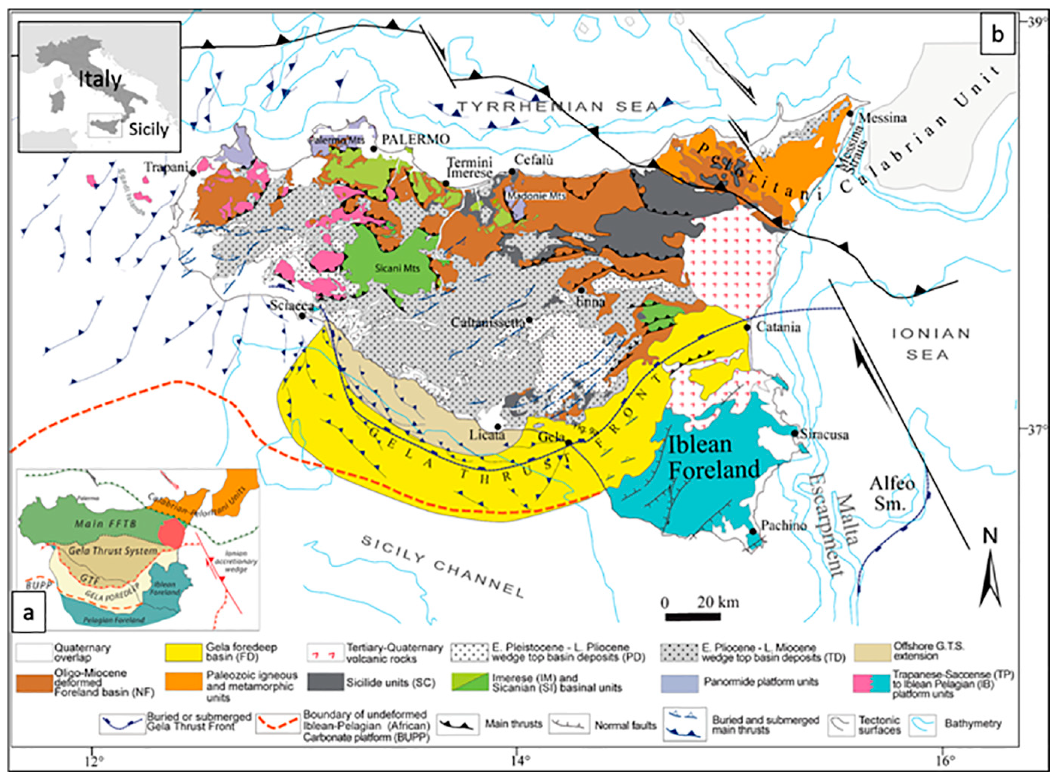
2. Study Area
3. Data Collection and Processing
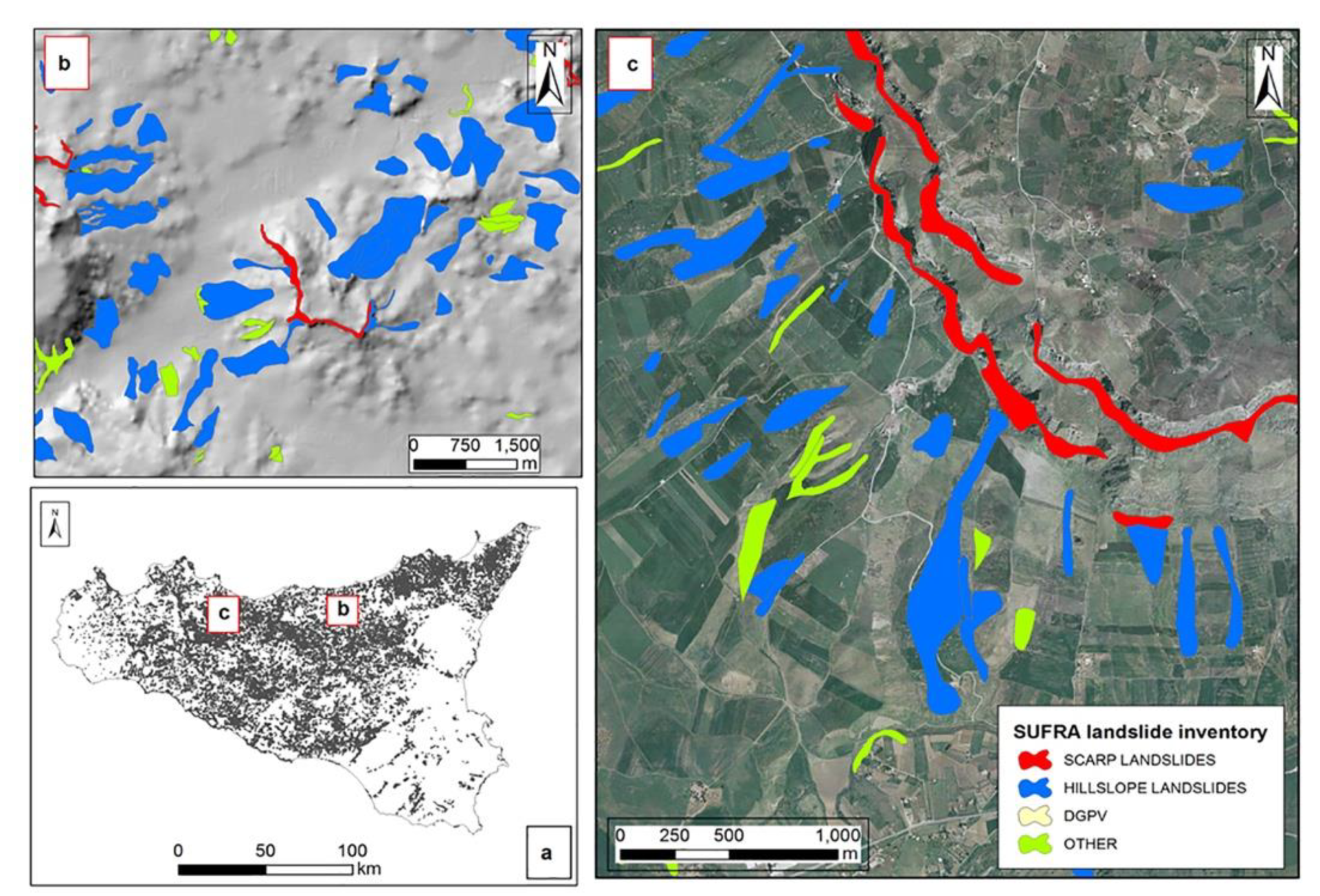
3.1. Landslide Inventory
3.2. Modelling Approach
3.3. Conditional Analysis (CA)
3.4. Binary Logistic Regression (BLR)
3.5. Variables Selection and Factor Class Definition
3.5.1. Continuous Variables
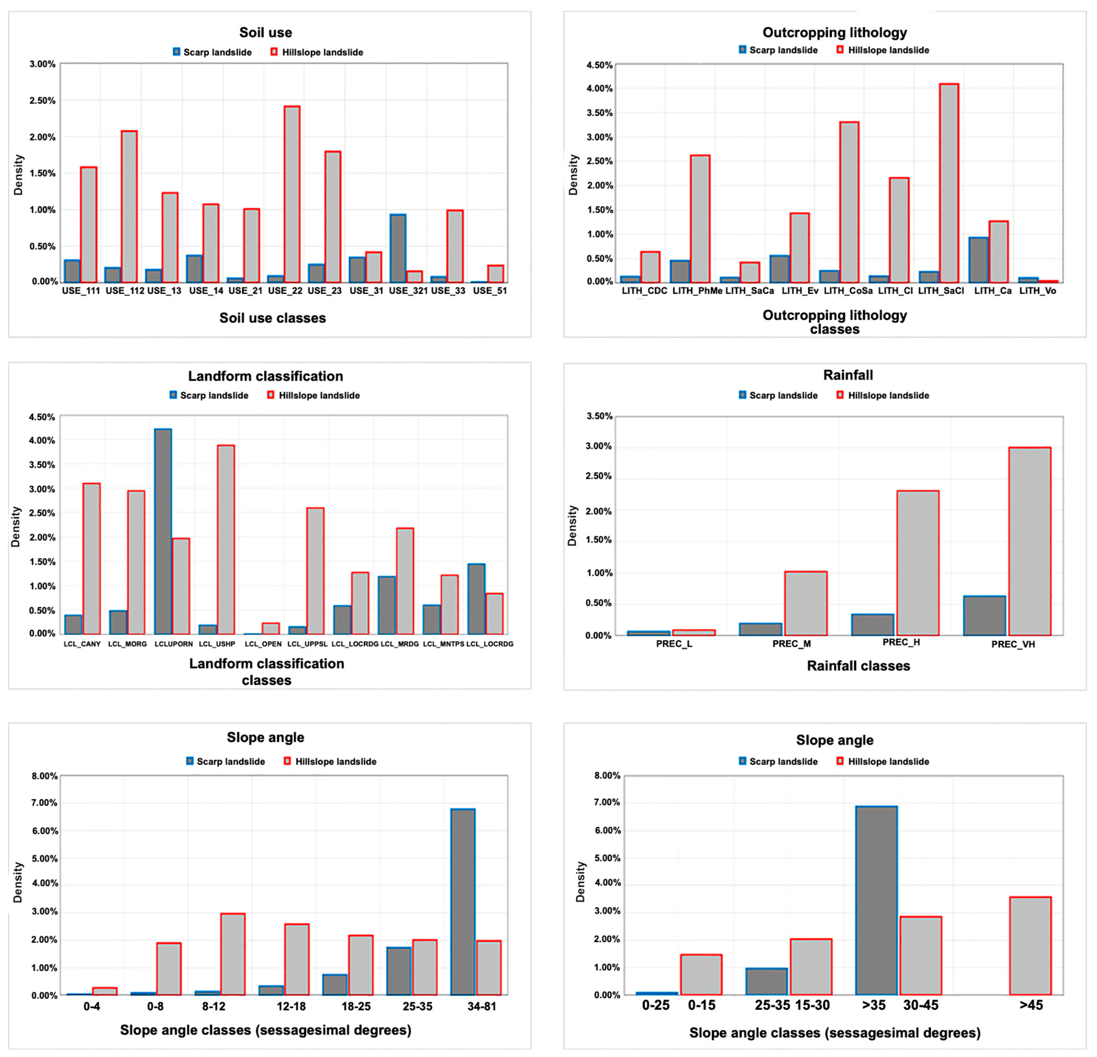
- Slope angle (SLO) is usually considered as one of the main controlling factors in landslide modelling. At first, SLO was classified into 5 natural break intervals [14], expressed in sexagesimal degrees (0°–5°; 5°–12°; 12°–18°–18°–32°: > 32°). The raster-file of the slope angle was obtained by resampling the 2-meter resolution ARTA-DTM flight ATA (2007/2009) to 100 m per side. As shown in Figure 3, the proposed reclassification for the slope angle for the hillslope landslide does not reveal the theoretical concept for the slope increase, which corresponds to an increase in the likelihood of landslides occurring. This does not happen with the scarp landslide, where increasing the slope angle leads to an increase in the percentage of landslides.
3.5.2. Category Variables
- Landform classification (LCL). Using an ArcMap open source tool, the LCL variable was derived directly from the DEM. LCL provides a simple and repeatable method to classify the landscape into slope position and landform category comparison. The different landform category classes can be determined by classifying the combination of a small and large neighborhood topographic position index (TPI) computed for each cell from different scales. The TPI is simply the difference between a cell elevation value and the average elevation of the neighborhood around that cell. Positive values mean the cell is higher than its surroundings, while negative values mean it is lower [61]. To compute the LCL, the small and the large neighborhood areas were set to 500 and 100 m, respectively. Ten landform classes were thus obtained (Table 2);
- Outcropping lithology (LITH). Together with the slope itself, the lithological conditions of an area are the most important factors influencing the geomorphological processes on the slope. The lithology controls the response of the slope in terms of the trigger-time of the collapse because of rainfall or seismic forces and evolution of the process. The lithotypes cropping out in the map of the Sicilian region were used in this research and grouped into 9 different “lithological complexes”, according to their geotechnical characteristics. The output lithological complexes were named as shown in Table 2. The clay complex is the most widespread one in the Sicilian territory, as it crops out in almost 35% of the area (more than 50,000 hectares);
- Soil use (USE). In this test, we used a soil use map derived from the 1:100,000 Corine Land Cover project (2006) based on a revised version of the Corine Land Cover 2000 dataset with the results of Landsat 1988 and photointerpretation of aerial photos. Table 2 shows land cover characteristics in 11 different classes, for terrain units larger than 0.25 km2. The Corine 2006 map was converted into a soil cover digital map provided by the Sicilian region, using the second level of the Corine legend, except for the “urban areas” class, which has been divided into continuous (USE_111) and discontinuous (USE_112) urban fabric, corresponding to level III of the Corine Land Cover classification. Arable land (USE_21) covers more than 30% of the research area. Forest crops cover about 7% of the area and mainly appear in the northeastern sectors. Areas covered by shrubby and herbaceous vegetation associations are dispersed around the study area: they cover 17%. Urban area cover is only 4.5%;
- Rainfall (RAIN). For rainfall, 280 rainfall stations were used to create the GRID rainfall map using the inverse distance weighted method. The database from the Sicilian regional administration office (http://www.osservatoriodelleacque.it) was used to extract the mean annual precipitation (for the period 1921–2009). Regarding precipitation, Sicily can be divided into three main sectors with three different pluviometric regimes: the northern sector: includes all the Tyrrhenian coast of the island. Rainfall here is characterized by a rainy season (autumn–winter) and a dry spring and summer. Eastern Sicily: in this area, rainfall is also greater in winter. Precipitation is often concentrated into short spells and is sometimes very violent. This is because the precipitation depression bearers come from Africa and are very hot and humid, favoring strong thermal contrasts. Southern Sicily: includes all the area bordered by the Mediterranean Sea. As in the rest of the island, winter is the rainy season. The number of rainy days is less than in the northern area (<60 days per year). In some areas, rainfall is sparse, especially in the coastal zone. The areas with the highest rainfall are the Madonie, Nebrodi, and Peloritani peaks, Etna, and the area south of Palermo. The driest areas are the Plain of Catania and the southern coast, in particular, Gela city.
4. Model-Building Strategy
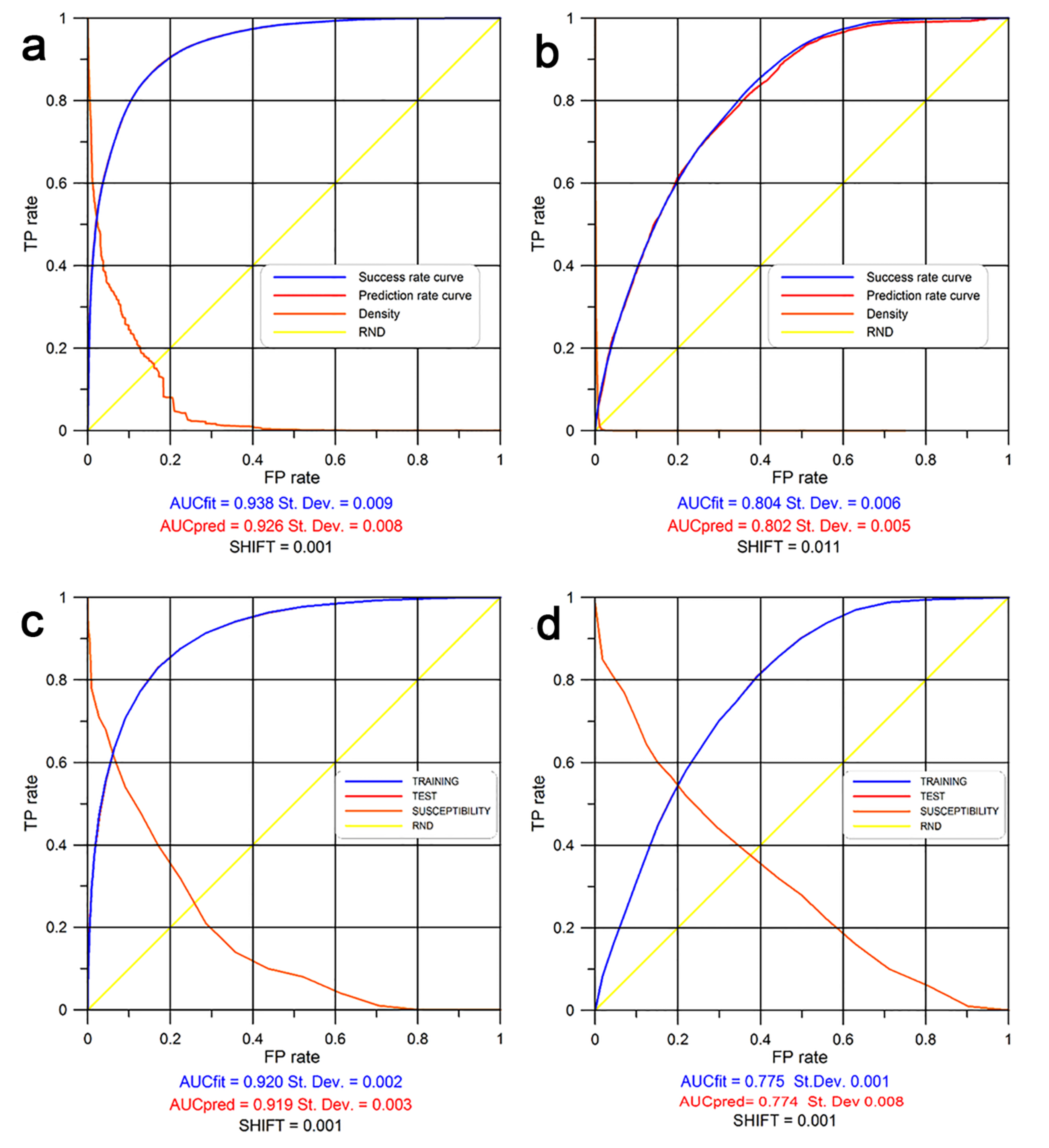
5. Results and Validation
6. Discussion
7. Final Remarks and Management Implications
Author Contributions
Funding
Conflicts of Interest
References
- Guzzetti, F.; Carrara, A.; Cardinali, M.; Reichenbach, P. Landslide hazard evaluation: A review of current techniques and their application in a multi-scale study, Central Italy. Geomorphology 1999, 31, 181–216. [Google Scholar] [CrossRef]
- Guzzetti, F.; Reichenbach, P.; Cardinali, M.; Galli, M.; Ardizzone, F. Probabilistic landslide hazard assessment at the basin scale. Geomorphology 2005, 72, 272–299. [Google Scholar] [CrossRef]
- Brabb, E.E. Innovative approach to landslide hazard and risk mapping. In Proceedings of the 4th International Symposium on Landslides, Toronto, ON, Canada, 16–21 September 1984; Volume 1, pp. 307–324. [Google Scholar]
- Soeters, R.; van Westen, C.J. Slope instability recognition, analysis, and zonation. In Landslides Investigation and Mitigation; Special Report 247; Transportation Research Board: Washington, DC, USA, 1996; pp. 129–177. [Google Scholar]
- Lyell, C. Principles of Geology, Being an Attempt to Explain the Former Changes of the Earth’s Surface, by Reference to Causes Now in Operation; John Murray: London, UK, 1833; Volume 3. [Google Scholar]
- Aleotti, P.; Chowdhury, R. Landslide hazard assessment: Summary review and new perspectives. Bull. Eng. Geol. Environ. 1999, 58, 21–44. [Google Scholar] [CrossRef]
- Carrara, A.; Cardinali, M.; Detti, R.; Guzzetti, F.; Reichenbach, P. Gis techniques and statistical models in evaluating landslide-hazard. Earth Surf. Process. Landf. 1991, 16, 427–445. [Google Scholar] [CrossRef]
- Varnes, D.J. Slope movements, type and processes. In Landslides Analysis and Control; Schuster, R.L., Krizek, R.J., Eds.; Special Report 176; Transportation Research Board: Washington, DC, USA, 1984. [Google Scholar]
- Cascini, L. Applicability of landslide susceptibility and hazard zoning at different scales. Eng. Geol. 2008, 102, 164–177. [Google Scholar] [CrossRef]
- Hervás, J.; Günther, A.; Reichenbach, P.; Chacón, J.; Pasuto, A.; Malet, J.-P.; Trigila, A.; Hobbs, P.; Maquaire, O.; Tagliavini, F.; et al. Recommendations on a common approach for mapping areas at risk of landslides in Europe. In Guidelines for Mapping Areas at Risk of Landslides in Europe; Hervás, J., Ed.; JRC Report EUR 23093 EN; Office for Official Publications of the European Communities: Luxembourg, 2007; 53p. [Google Scholar]
- Eckelmann, W.; Baritz, R.; Bialousz, S.; Carre, F.; Jones, B.; Kibblewhite, M.; Kozak, J.; Le Bas, C.; Tóth, G.; Várallyay, G.; et al. Common Criteria for Risk Area Identification according to Soil Threats; European Soil Bureau Research Report No.20, EUR 22185 EN; Office for Official Publications of the European Communities: Luxembourg, 2006; 94p. [Google Scholar]
- Glade, T.; Reichenbach, P.; Resources, N. Preface “Landslide hazard and risk assessment at different scales”. Nat. Hazards Earth Syst. Sci. 2013, 13, 2169–2171. [Google Scholar]
- Günther, A.; Reichenbach, P.; Malet, J.; Van Den Eeckhaut, M.; Hervás, J.; Dashwood, C.; Guzzetti, F. Tier-based approaches for landslide susceptibility assessment in Europe. Landslides 2012, 10, 529–546. [Google Scholar] [CrossRef]
- Manzo, G.; Tofani, V.; Segoni, S.; Battistini, A.; Catani, F. GIS techniques for regional-scale landslide susceptibility assessment: The Sicily (Italy) case study. Int. J. Geogr. Inf. Sci. 2013, 27, 1433–1452. [Google Scholar] [CrossRef]
- ARTA_Sicilia. Piano Stralcio di bacino per l’Assetto Idrogeologico Della Regione Siciliana; Assessorato Regionale Territorio e Ambiente della Regione Sicilia: Sicilia, Italy, 2004; 165p. [Google Scholar]
- Agnesi, V.; Di Maggio, C.; Macaluso, T. Morphostructural setting and geomorphological evolution in the Madonie Mountains (Northern Sicily, Italy). Suppl. Geogr. Fis. Din. Quat. 1997, 3, 43–44. [Google Scholar]
- Catalano, R.; Agate, M.; Albanese, C.; Avellone, G.; Basilone, L.; Morticelli, G.; Gugliotta, C.; Sulli, A.; Valenti, V.; Gibilaro, C.; et al. Walking along a Crustal Profile Across the Sicily Fold and Thrust Belt; Geological Field Trips: Palermo, IT, USA, 2013; Volume 5. [Google Scholar]
- Di Maggio, C.; Madonia, G.; Parise, M.; Vattano, M. Karst of Sicily and its conservation. J. Cave Karst Stud. 2012, 74, 157–172. [Google Scholar] [CrossRef]
- Dikau, R.; Brunsden, D.; Schrott, L.; Ibsen, M. Landslide Recognition. Identification, Movement and Courses; Report No. 1 of the European Commission Environment Programme; Wiley and Sons: Chichester, UK, 1996; 251p. [Google Scholar]
- Cruden, D.M. A simple definition of a landslide. Bull. Int. Assoc. Eng. Geol. 1991, 43, 27–29. [Google Scholar] [CrossRef]
- Cruden, D.M.; Varnes, D.J. Landslides Types and Processes. In Landslides: Investigation and Mitigation; Special Report 247; Transportation Research Board: Washington, DC, USA, 1996; pp. 36–75. [Google Scholar]
- Guzzetti, F.; Reichenbach, P.; Ardizzone, F.; Cardinali, M.; Galli, M. Estimating the quality of landslide susceptibility models. Geomorphology 2006, 81, 166–184. [Google Scholar] [CrossRef]
- Bosi, C.; Dramis, F.; Gentili, B. Carte geomorfologiche di dettaglio e carte di stabilita: Esempi nel territorio marchigiano. Geol. Appl. Idrogeol. 1982, 20, 53–62. [Google Scholar]
- Chacón, J.; Irigaray, C.; Fernández, T.; El Hamdouni, R. Engineering geology maps: Landslides and geographical information systems. Bull. Eng. Geol. Environ. 2006, 65, 341–411. [Google Scholar] [CrossRef]
- Carrara, A.; Guzzetti, F.; Cardinali, M.; Reichenbach, P. Use of GIS technology in the prediction and monitoring of landslide hazard. Nat. Hazards 1999, 20, 117–135. [Google Scholar] [CrossRef]
- Carrara, A.; Cardinali, M.; Guzzetti, F.; Reichenbach, P. GIS technology in mapping landslide hazard. In Geographical Information Systems in Assessing Natural Hazards; Carrara, A., Guzzetti, F., Eds.; Kluwer Academic Publishers: Dordrecht, The Netherlands, 1995; pp. 135–175. [Google Scholar]
- Irigaray, C.; Fernández, T.; El Hamdouni, R.; Chacón, J. Evaluation and validation of landslide-susceptibility maps obtained by a GIS matrix method: Examples from the Betic Cordillera (southern Spain). Nat. Hazards 2007, 41, 61–79. [Google Scholar] [CrossRef]
- Carrara, A.; Crosta, G.; Frattini, P. Comparing models of debris-flow susceptibility in the alpine environment. Geomorphology 2008, 94, 353–378. [Google Scholar] [CrossRef]
- Lombardo, L.; Cama, M.; Maerker, M.; Rotigliano, E. A test of transferability for landslides susceptibility models under extreme climatic events: Application to the Messina 2009 disaster. Nat. Hazards 2014, 74, 1951–1989. [Google Scholar] [CrossRef]
- Rossi, M.; Guzzetti, F.; Reichenbach, P.; Mondini, A.C.; Peruccacci, S. Optimal landslide susceptibility zonation based on multiple forecasts. Geomorphology 2010, 114, 129–142. [Google Scholar] [CrossRef]
- Van Den Eeckhaut, M.; Hervás, J.; Jaedicke, C.; Malet, J.P.; Montanarella, L.; Nadim, F. Statistical modelling of Europe-wide landslide susceptibility using limited landslide inventory data. Landslides 2011, 9, 357–369. [Google Scholar] [CrossRef]
- Clerici, A.; Perego, S.; Tellini, C.; Vescovi, P. Landslide failure and runout susceptibility in the upper T. Ceno valley (Northern Apennines, Italy). Nat. Hazards 2009, 52, 1–29. [Google Scholar] [CrossRef]
- Conoscenti, C.; Di Maggio, C.; Rotigliano, E. GIS analysis to assess landslide susceptibility in a fluvial basin of NW Sicily (Italy). Geomorphology 2008, 94, 325–339. [Google Scholar] [CrossRef]
- Costanzo, D.; Cappadonia, C.; Conoscenti, C.; Rotigliano, E. Exporting a Google EarthTM aided earth-flow susceptibility model: A test in central Sicily. Nat. Hazards 2011, 61, 103–114. [Google Scholar] [CrossRef]
- Costanzo, D.; Rotigliano, E.; Irigaray, C.; Jiménez-Perálvarez, J.D.; Chacón, J. Factors selection in landslide susceptibility modelling on large scale following the gis matrix method: Application to the river Beiro basin (Spain). Nat. Hazards Earth Syst. Sci. 2012, 12, 327–340. [Google Scholar] [CrossRef]
- Costanzo, D.; Chacón, J.; Conoscenti, C.; Irigaray, C.; Rotigliano, E. Forward logistic regression for earth-flow landslide susceptibility assessment in the Platani river basin (southern Sicily, Italy). Landslides 2014, 11, 639–653. [Google Scholar] [CrossRef]
- Lombardo, L.; Cama, M.; Conoscenti, C.; Marker, M.; Rotigliano, E. Binary logistic regression versus stochastic gradient boosted decision trees in assessing landslide susceptibility for multiple-occurring landslide events: Application to the 2009 storm event in Messina (Sicily, southern Italy). Nat. Hazards 2015, 79, 1621–1648. [Google Scholar] [CrossRef]
- Rotigliano, E.; Agnesi, V.; Cappadonia, C.; Conoscenti, C. The role of the diagnostic areas in the assessment of landslide susceptibility models: A test in the sicilian chain. Nat. Hazards 2011, 58, 981–999. [Google Scholar] [CrossRef]
- Rotigliano, E.; Cappadonia, C.; Conoscenti, C.; Costanzo, D.; Agnesi, V. Slope units-based flow susceptibility model: Using validation tests to select controlling factors. Nat. Hazards 2012, 61, 143–153. [Google Scholar] [CrossRef]
- Clerici, A.; Perego, S.; Tellini, C.; Vescovi, P. A GIS-based automated procedure for landslide susceptibility mapping by the Conditional Analysis method: The Baganza valley case study (Italian Northern Apennines). Environ. Geol. 2006, 50, 941–961. [Google Scholar] [CrossRef]
- Vergari, F.; Della Seta, M.; Del Monte, M.; Fredi, P.; Lupia Palmieri, E. Landslide susceptibility assessment in the Upper Orcia Valley. Nat. Hazards Earth Syst. Sci. 2011, 11, 1475–1495. [Google Scholar] [CrossRef]
- Davis, J.C. Statistics and Data Analysis in Geology; John Wiley & Sons Inc.: New York, NY, USA, 1973; 564p. [Google Scholar]
- Chung, C.F.; Fabbri, A.G. Validation of Spatial Prediction Models for Landslide Hazard Mapping. Nat. Hazards 2003, 30, 451–472. [Google Scholar] [CrossRef]
- Jiménez-Perálvarez, J.D.; Irigaray, C.; El Hamdouni, R.; Chacón, J. Landslide-susceptibility mapping in a semi-arid mountain environment: An example from the southern slopes of Sierra Nevada (Granada, Spain). Bull. Eng. Geol. Environ. 2010, 70, 265–277. [Google Scholar] [CrossRef]
- Santacana, N.; Baeza, B.; Corominas, J.; De Paz, A.; Marturiá, J. A GIS-Based Multivariate Statistical Analysis for Shallow Landslide Susceptibility Mapping in La Pobla de Lillet Area (Eastern Pyrenees, Spain). Nat. Hazards 2003, 30, 281–295. [Google Scholar] [CrossRef]
- Hosmer, D.W.; Lemeshow, S. Interpretation of the fitted logistic regression model. In Applied Logistic Regression, 2nd ed.; John Wiley & Sons, Inc.: New York, NY, USA, 2000; pp. 47–90. [Google Scholar]
- Akgün, A.; Türk, N. Mapping erosion susceptibility by a multivariate statistical method: A case study from the Ayvalik region, NW Turkey. Comput. Geosci. 2011, 37, 1515–1524. [Google Scholar] [CrossRef]
- Ayalew, L.; Yamagishi, H. The application of GIS-based logistic regression for landslide susceptibility mapping in the Kakuda-Yahiko Mountains, Central Japan. Geomorphology 2005, 65, 15–31. [Google Scholar] [CrossRef]
- Kavzoglu, T.; Sahin, E.K.; Colkesen, I. Landslide susceptibility mapping using GIS-based multi-criteria decision analysis, support vector machines, and logistic regression. Landslides 2013, 11, 425–439. [Google Scholar] [CrossRef]
- Van Den Eeckhaut, M.; Hervás, J. State of the art of national landslide databases in Europe and their potential for assessing landslide susceptibility, hazard and risk. Geomorphology 2012, 139–140, 545–558. [Google Scholar] [CrossRef]
- Dai, F.C.; Lee, C.F.; Li, J.; Xu, Z.W. Assessment of landslide susceptibility on the natural terrain of Lantau Island, Hong Kong. Environ. Geol. 2001, 40, 381–391. [Google Scholar]
- Kim, G.; Lee, J.; Lee, K. Application of representative elementary area (REA) to lineament density analysis for groundwater implications. Water Resour. 2004, 8, 27–42. [Google Scholar] [CrossRef]
- Dai, F.C.; Lee, C.F. Landslide characteristics and slope instability modeling using GIS, Lantau Island, Hong Kong. Geomorphology 2020, 42, 213–228. [Google Scholar] [CrossRef]
- Rakotomalala, R. TANAGRA: A free software for research and academic purposes. In Proceedings of the European Grid Conference, Amsterdam RNTI-E-3, Amsterdam, The Netherlands, 5 February 2005; Volume 2, pp. 697–702. [Google Scholar]
- Crozier, M.J. Field assessment of slope instability. In Slope Instability; Brunsden, D., Prior, D.B., Eds.; John Wiley & Sons: Chichester, UK, 1984; pp. 103–142. [Google Scholar]
- Hansen, A. Landslide hazard analysis. In Slope Instability; Brunsden, D., Prior, D.B., Eds.; John Wiley & Sons: Chichester, UK, 1984; pp. 523–602. [Google Scholar]
- Palenzuela, J.A.; Jiménez-Perálvarez, J.D.; Chacón, J.; Irigaray, C. Assessing critical rainfall thresholds for landslide triggering by generating additional information from a reduced database: An approach with examples from the Betic Cordillera (Spain). Nat. Hazards 2016, 84, 185–212. [Google Scholar] [CrossRef]
- Jenness, J. Topographic Position Index (TPI) v. 1.3a. Jenness Enterprises. 2006. Available online: http://www.jennessent.com/arcview/tpi.htm (accessed on 8 June 2020).
- Regmi, N.R.; Giardino, J.R.; McDonald, E.V.; Vitek, J.D. A comparison of logistic regression-based models of susceptibility to landslides in western Colorado, USA. Landslides 2013, 11, 247–262. [Google Scholar] [CrossRef]
- Hanley, A.J.; McNeil, J.B. The Meaning and Use of the Area under a Receiver Operating Characteristic (ROC) Curve. Radiology 1982, 143, 29–36. [Google Scholar] [CrossRef] [PubMed]
- Fawcett, T. An introduction to ROC analysis. Pattern Recognit. Lett. 2006, 27, 861–874. [Google Scholar] [CrossRef]
- Nandi, A.; Shakoor, A. A GIS-based landslide susceptibility evaluation using bivariate and multivariate statistical analyses. Eng. Geol. 2010, 110, 11–20. [Google Scholar] [CrossRef]
- Frattini, P.; Crosta, G.; Carrara, A. Techniques for evaluating the performance of landslide susceptibility models. Eng. Geol. 2010, 111, 62–72. [Google Scholar] [CrossRef]
- Lasko, T.A.; Bhagwat, J.G.; Zou, K.H.; Ohno-Machado, L. The use of receiver operating characteristic curves in biomedical informatics. J. Biomed. Inform. 2005, 38, 404–415. [Google Scholar] [CrossRef] [PubMed]
- Goodenough, D.J.; Rossmann, K.; Lusted, L.B. Radiographic applications of receiver operating characteristic (ROC) curves. Radiology 1974, 110, 89–95. [Google Scholar] [CrossRef]
- Egan, J.P. Signal Detection Theory and ROC Analysis; Academic Press: New York, NY, USA, 1975; 277p. [Google Scholar]
- Williams, C.J.; Lee, S.S.; Fisher, R.A.; Dickerman, L.H. A comparison of statistical methods for prenatal screening for Down syndrome. Appl. Stoch. Models Data Anal. 1999, 15, 89–101. [Google Scholar] [CrossRef]
- Nefeslioglu, H.A.; Gokceoglu, C.; Sonmez, H. An assessment on the use of logistic regression and artificial neural networks with different sampling strategies for the preparation of landslide susceptibility maps. Eng. Geol. 2008, 97, 171–191. [Google Scholar] [CrossRef]
- Ohlmacher, G.C.; Davis, J.C. Using multiple logistic regression and GIS technology to predict landslide hazard in northeast Kansas, USA. Eng. Geol. 2003, 69, 331–343. [Google Scholar] [CrossRef]
- Chung, C.F.; Fabbri, A.G.; Van Westen, C.J. Multivariate regression analysis for landslide hazard zonation. In Geographical Information Systems in Assessing Natural Hazards; Carrara, A., Guzzetti, F., Eds.; Kluwer Academic Publishers: Dordrecht, The Netherlands, 1995; pp. 107–133. [Google Scholar]
- Atckinson, P.M.; Massari, R. Generalised linear modelling of susceptibility lo landsliding in the Central Apennines, Italy. Comput. Geosci. 1998, 24, 373–385. [Google Scholar] [CrossRef]
- Irigaray, C.; Fernández, T.; El Hamdouni, R.; Chacón, J. Verification of landslide susceptibility mapping: A case study. Earth Surf. Process. Landf. 1999, 24, 537–544. [Google Scholar]
- Fernández, T.; Irigaray, C.; El Hamdouni, R.; Chacon, J. Methodology for landslide susceptibility mapping by means of a GIS. Application to the Contraviesa area (Granada, Spain). Nat. Hazard 2003, 30, 297–308. [Google Scholar]
- Remondo, J.; Gonzalez, A.; Diaz De Teran, J.R.; Cendrero, A.; Fabbri, A.; Chung, C.F. Validation of landslide susceptibility maps; examples and applications from a case study in Northern Spain. Nat. Hazards 2003, 30, 437–449. [Google Scholar] [CrossRef]
- Plattner, T. Modelling public risk evaluation of natural hazards: A conceptual approach. Nat. Hazards Earth Syst. Sci. 2005, 5, 357–366. [Google Scholar] [CrossRef]


| PAI | Number of Cases | Area [m2] for a Single Landslide | Total (km2) | Percentages | SUFRA | ||||||
|---|---|---|---|---|---|---|---|---|---|---|---|
| TYPOLOGY | max | min | mean | Std. Dev. | Landslide Area | Total Area | Number of Cases | Area (km2) | TYPOLOGY | ||
| 1. Falls/Topples | 5460 | 1,630,259 | 25 | 15,310 | 1,138,586 | 84 | 6.4 | 0.3 | 5460 | 84 | 1. Scarp Landslide |
| 2. Rapid flows | 853 | 1,152,779 | 79 | 15,403 | 48,938 | 13 | 1.0 | 0.1 | 10,202 | 435 | 2. Hillslope landslide |
| 4. Slides | 2835 | 45,106 | 530 | 11,350 | 11,987 | 81 | 6.2 | 0.3 | |||
| 5. Complex | 3076 | 735,524 | 766 | 50,290 | 114,782 | 215 | 16.5 | 0.8 | |||
| 7. Slow flow | 3438 | 194,381 | 869 | 34,263 | 41,727 | 125 | 9.6 | 0.5 | |||
| 6. DPGV/Spreads | 28 | 7,891,513 | 212 | 509,802 | 509,802 | 14 | 1.1 | 0.1 | 28 | 14 | 3. DPGV and Spreads |
| 3. Sinkhole | 43 | 1,380,425 | 25 | 51,918 | 219,976 | 2 | 0.2 | 0.0 | 17,404 | 772 | 4. Others |
| 8. Areas with diffused landslides | 2877 | 225,203 | 1482 | 53,560 | 225,203 | 288 | 22.1 | 1.1 | |||
| 9. Slowly surface deformation | 3512 | 124,610 | 605 | 23,534 | 29,059 | 155 | 11.9 | 0.6 | |||
| 10. Badlands | 1266 | 1,625,318 | 3471 | 42,755 | 302,626 | 54 | 4.1 | 0.2 | |||
| 11. Caused by accel. erosion | 9706 | 254,775 | 9358 | 30,171 | 57,136 | 273 | 20.9 | 1.1 | |||
| Total | 33,094 | 2,699,822 | 1305 | 100.0 | 5.1 | 33,094 | 1305 | Total | |||
| Area of Sicily 25.832 Km2 | |||||||||||
| Categorical Variables | ||||
|---|---|---|---|---|
| Variable | References | Description | Code | Percentage Distribution (%) |
| Soil Use | (Corine Land Cover project, 2006) | Continuous urban fabric | USE_111 | 1.94 |
| Discontinous urban fabric | USE_112 | 2.42 | ||
| Transitional areas | USE_13 | 0.27 | ||
| Green urban areas | USE_14 | 0.06 | ||
| Arable land | USE_21 | 32.54 | ||
| Permanent crops | USE_22 | 21.61 | ||
| Heterogeneous agricultural areas | USE_23 | 14.97 | ||
| Forest | USE_31 | 7.79 | ||
| Shrub and/or herbaceous associations | USE_32 | 17.31 | ||
| Open spaces with little or no vegetation | USE_33 | 0.65 | ||
| Water bodies | USE_51 | 0.44 | ||
| Outcropping lithology | Lithological Complex | Continental clastic deposition complex | LITH_CDC | 12.94 |
| Phyllitic and metamorphic complex | LITH_PhMe | 3.51 | ||
| Sandy-calcarenitic complex | LITH_SaCa | 13.22 | ||
| Evapotitic complex | LITH_Ev | 4.86 | ||
| Conglomerate-sandstone | LITH_CoSa | 2.74 | ||
| Clay complex | LITH_Cl | 34.13 | ||
| Sandstone and clay | LITH_SaCl | 8.66 | ||
| Carbonatic complex | LITH_Ca | 13.41 | ||
| Volcanic complex | LITH_Vo | 6.53 | ||
| Landform classification | Landform Classification (Weiss, 2001) | Canyons | LCL_CANY | 7.51 |
| Midslope drainage | LCL_MDRG | 2.27 | ||
| Upland drainage | LCL_UPDRN | 2.32 | ||
| U-shaped valleys | LCL_USHP | 2.92 | ||
| Plains | LCL_PLAINS | 32.58 | ||
| Open slopes | LCL_OPEN | 39.51 | ||
| Upper slope | LCL_UPPSL | 2.80 | ||
| Local ridge | LCL_LOCRDG | 0.00 | ||
| Midslope ridge | LCL_MRDG | 2.00 | ||
| Mountain tops | LCL_MNTPS | 8.07 | ||
| Rainfall (mm) | SIAS, 2015 | 0–450 | RAIN_L | 1.58 |
| 450–600 | RAIN_M | 63.32 | ||
| 600–800 | RAIN_H | 20.75 | ||
| >800 | RAIN_VH | 14.34 | ||
| Slope Angle (Scarp landslide) | Θ = TAN Δy/Δx | Canyons | SLO_L | 87.81 |
| Midslope drainage | SLO_M | 10.72 | ||
| Upland drainage | SLO_H | 1.47 | ||
| Slope Angle (Hillslope landslide) | U-shaped valleys | SLO_L | 78.09 | |
| Plains | SLO_M | 15.28 | ||
| Open slopes | SLO_H | 6.43 | ||
| Upper slope | SLO_VH | 0.20 | ||
| Most diffused UCUs for SCR_LSN | |||||||
| UCU Code | Area (Ha) | LCL | LITH | USE | SLO | RAIN | δ |
| 1502 | 2 | LCL_MNTPS | LITH_Ca | USE_112 | SLO_VH | RAIN_VH | 100.00% |
| 1515 | 3 | LCL_UPDRN | LITH_Ca | USE_23 | SLO_VH | RAIN_VH | 100.00% |
| 1204 | 8 | LCL_USHP | LITH_SaCa | USE_13 | SLO_H | RAIN_H | 100.00% |
| 1517 | 3 | LCL_MNTPS | LITH_Ca | USE_13 | SLO_H | RAIN_L | 100.00% |
| 1217 | 3 | LCL_MNTPS | LITH_Ca | USE_13 | SLO_VH | RAIN_VH | 100.00% |
| 1001 | 2 | LCL_UPDRN | LITH_SaCa | USE_13 | SLO_H | RAIN_VH | 100.00% |
| 4095 | 1 | LCL_USHP | LITH_CoSa | USE_13 | SLO_M | RAIN_H | 100.00% |
| 1075 | 2 | LCL_UPDRN | LITH_Ca | USE_13 | SLO_VH | RAIN_M | 100.00% |
| 3403 | 1 | LCL_USHP | LITH_Ca | USE_13 | SLO_VH | RAIN_M | 100.00% |
| 3850 | 3 | LCL_UPDRN | LITH_CoSa | USE_112 | SLO_H | RAIN_VH | 100.00% |
| Most diffused UCUs for HILL_LSN | |||||||
| UCU Code | Area (Ha) | LCL | LITH | USE | SLO | RAIN | δ |
| 2778 | 14 | LCL_OPEN | LITH_CI | USE_13 | SLO_VH | RAIN_VH | 100.00% |
| 3230 | 11 | LCL_UPDRN | LITH_CI | USE_21 | SLO_H | RAIN_H | 89.00% |
| 2759 | 34 | LCL_OPEN | LITH_CI | USE_21 | SLO_L | RAIN_M | 62.00% |
| 2777 | 17 | LCL_OPEN | LITH_CI | USE_13 | SLO_VH | RAIN_M | 57.00% |
| 3370 | 13 | LCL_UPDRN | LITH_CI | USE_32 | SLO_VH | RAIN_VH | 36.00% |
| 2711 | 45 | LCL_OPEN | LITH_CI | USE_13 | SLO_H | RAIN_VH | 31.00% |
| 4376 | 14 | LCL_OPEN | LITH_SaCa | USE_21 | SLO_H | RAIN_H | 25.00% |
| 2735 | 32 | LCL_OPEN | LITH_CI | USE_13 | SLO_M | RAIN_L | 24.00% |
| 1272 | 14 | LCL_UPDRN | LITH_SaCa | USE_21 | SLO_M | RAIN_VH | 24.00% |
| 3381 | 7 | LCL_USHP | LITH_CI | USE_32 | SLO_VH | RAIN_VH | 23.00% |
| (a) | TEST SUBSET-PREDICTION SKILL | ||||||||||
| PREDICTED YES | PREDICTED NO | RECALL | FALL-OUT | ERROR RATE | AUC | ||||||
| YES | NO | YES | NO | YES TP/oP | NO TN/oN | YES FP/pP | NO FN/pN | ||||
| MODELS | 1 | 13,648 | 2850 | 3011 | 13,861 | 0.819 | 0.829 | 0.173 | 0.178 | 0.176 | 0.916 |
| 2 | 13,672 | 2853 | 3008 | 13,837 | 0.820 | 0.829 | 0.173 | 0.179 | 0.176 | 0.916 | |
| 3 | 13,849 | 2686 | 2831 | 14,004 | 0.830 | 0.839 | 0.162 | 0.168 | 0.165 | 0.921 | |
| 4 | 13,802 | 2634 | 2878 | 14,056 | 0.827 | 0.842 | 0.160 | 0.170 | 0.165 | 0.923 | |
| 5 | 13,686 | 2814 | 2994 | 13,876 | 0.821 | 0.831 | 0.171 | 0.177 | 0.174 | 0.917 | |
| 6 | 13,735 | 2743 | 2945 | 13,947 | 0.823 | 0.836 | 0.166 | 0.174 | 0.170 | 0.919 | |
| 7 | 13,732 | 2817 | 2948 | 13,873 | 0.823 | 0.831 | 0.170 | 0.175 | 0.173 | 0.917 | |
| 8 | 13,794 | 2755 | 2896 | 13,935 | 0.826 | 0.835 | 0.166 | 0.172 | 0.169 | 0.918 | |
| 9 | 13,790 | 2622 | 2890 | 14,068 | 0.827 | 0.843 | 0.160 | 0.170 | 0.165 | 0.923 | |
| 10 | 13,781 | 2688 | 2902 | 14,002 | 0.826 | 0.839 | 0.163 | 0.172 | 0.168 | 0.917 | |
| ALL | 13,748.9 | 2746.2 | 2930.3 | 13,945.9 | 0.824 | 0.835 | 0.166 | 0.174 | 0.170 | 0.919 | |
| 65.1 | 86.2 | 60.9 | 83.6 | 0.004 | 0.005 | 0.005 | 0.004 | 0.004 | 0.003 | ||
| (b) | TEST SUBSET-PREDICTION SKILL | ||||||||||
| PREDICTED YES | PREDICTED NO | RECALL | FALL-OUT | ERROR RATE | AUC | ||||||
| YES | NO | YES | NO | YES TP/oP | NO TN/oN | YES FP/pP | NO FN/pN | ||||
| MODELS | 1 | 206,596 | 100,179 | 48,054 | 154,471 | 0.811 | 0.607 | 0.327 | 0.237 | 0.291 | 0.776 |
| 2 | 206,596 | 100,179 | 48,054 | 154,471 | 0.811 | 0.607 | 0.327 | 0.237 | 0.291 | 0.775 | |
| 3 | 207,100 | 100,614 | 47,550 | 154,036 | 0.813 | 0.605 | 0.327 | 0.236 | 0.291 | 0.776 | |
| 4 | 206,960 | 101,894 | 47,550 | 154,036 | 0.813 | 0.602 | 0.330 | 0.236 | 0.293 | 0.772 | |
| 5 | 206,275 | 99,734 | 48,375 | 154,916 | 0.810 | 0.608 | 0.326 | 0.238 | 0.291 | 0.776 | |
| 6 | 206,665 | 100,608 | 47,659 | 153,889 | 0.813 | 0.605 | 0.327 | 0.236 | 0.291 | 0.766 | |
| 7 | 206,991 | 100,761 | 47,659 | 153,889 | 0.813 | 0.604 | 0.327 | 0.236 | 0.291 | 0.775 | |
| 8 | 206,455 | 99,808 | 48,195 | 154,842 | 0.811 | 0.608 | 0.326 | 0.237 | 0.291 | 0.775 | |
| 9 | 206,755 | 101,015 | 47,895 | 153,635 | 0.812 | 0.603 | 0.328 | 0.238 | 0.292 | 0.773 | |
| 10 | 206,880 | 101,576 | 47,770 | 153,074 | 0.812 | 0.601 | 0.329 | 0.238 | 0.293 | 0.775 | |
| ALL | 206,727 | 100,636 | 47,876 | 154,125.9 | 0.811 | 0.604 | 0.327 | 0.237 | 0.292 | 0.774 | |
| 259.0 | 710.5 | 285.3 | 562.8 | 0.001 | 0.002 | 0.001 | 0.001 | 0.001 | 0.003 | ||
| FACTORS ANALYSIS | |||||||
|---|---|---|---|---|---|---|---|
| SCR_LSN | |||||||
| Attribute | Avg. (β) | Avg. (Std-dev) | Avg. Wald | Avg. Signif | Avg. OR | Avg. RK | n |
| SLO | 0.111 | 0.003 | 1046.925 | 0.0000 | 1.118 | 1.0 | 100 |
| LCL_MNTPS | 0.822 | 0.084 | 95.372 | 0.0000 | 2.281 | 2.0 | 100 |
| USE_321 | 0.977 | 0.070 | 195.690 | 0.0000 | 2.664 | 3.0 | 100 |
| USE_111 | 2.237 | 0.207 | 116.737 | 0.0000 | 9.419 | 4.7 | 100 |
| LCL_PLAINS | −2.071 | 0.164 | 159.161 | 0.0000 | 0.127 | 5.1 | 100 |
| LITH_Ca | 0.624 | 0.091 | 53.558 | 0.0000 | 1.886 | 8.3 | 100 |
| LITH_Ev | 0.934 | 0.120 | 63.700 | 0.0000 | 2.596 | 8.5 | 100 |
| USE_23 | 0.599 | 0.084 | 51.154 | 0.0000 | 1.827 | 9.4 | 100 |
| USE_112 | 1.571 | 0.220 | 51.222 | 0.0000 | 4.901 | 9.7 | 100 |
| LCL_OPEN | −0.562 | 0.072 | 61.954 | 0.0000 | 0.570 | 10.0 | 100 |
| LITH_SaCl | −0.644 | 0.111 | 37.426 | 0.0062 | 0.531 | 10.1 | 100 |
| LITH_PhMe | −0.898 | 0.143 | 42.396 | 0.0002 | 0.413 | 10.3 | 100 |
| LCL_USHP | −0.743 | 0.178 | 18.055 | 0.0005 | 0.480 | 13.8 | 100 |
| LITH_CDC | 0.650 | 0.130 | 25.732 | 0.0003 | 1.947 | 12.0 | 97 |
| USE_22 | 0.308 | 0.095 | 10.624 | 0.0024 | 1.362 | 15.2 | 52 |
| LITH_Cl | −0.028 | 0.106 | 5.054 | 0.2675 | 1.008 | 9.3 | 38 |
| LITH_CoSa | 0.576 | 0.179 | 10.373 | 0.0030 | 1.802 | 16.3 | 25 |
| LITH_SaCa | 0.329 | 0.156 | 7.230 | 0.1161 | 1.427 | 13.3 | 14 |
| FACTORS ANALYSIS | |||||||
|---|---|---|---|---|---|---|---|
| HILL_LSN | |||||||
| Attribute | Avg. (β) | Avg. (Std-dev) | Avg. Wald | Avg. Signif | Avg. OR | Avg. RK | n |
| LCL_PLAINS | −1.7649 | 0.0561 | 5788.5652 | 0.0050 | 0.1807 | 1.0 | 100 |
| RAIN_H | 0.0042 | 0.0001 | 3906.3562 | 0.0000 | 1.0042 | 2.0 | 100 |
| LITH_Cl | 4.2016 | 0.0893 | 2217.0432 | 0.0000 | 66.9131 | 3.0 | 100 |
| LITH_SaCl | 4.0756 | 0.0898 | 2062.8770 | 0.0000 | 58.9854 | 4.1 | 100 |
| LITH_CoSa | 4.3585 | 0.0930 | 2200.4857 | 0.0000 | 78.2727 | 4.9 | 100 |
| LITH_Ev | 4.0339 | 0.0927 | 1895.9701 | 0.0000 | 56.5819 | 6.0 | 100 |
| LCL_MNTPS | −0.5599 | 0.0548 | 775.7442 | 0.0334 | 0.6012 | 7.2 | 100 |
| USE_22 | −0.5557 | 0.0242 | 930.3611 | 0.0031 | 0.5768 | 8.0 | 100 |
| USE_31 | −0.7374 | 0.0296 | 930.1456 | 0.0000 | 0.4809 | 8.8 | 100 |
| LITH_PhMe | 3.6490 | 0.0927 | 1552.2501 | 0.0000 | 38.5212 | 10.4 | 100 |
| LITH_CDC | 3.6064 | 0.0919 | 1543.0805 | 0.0000 | 36.8982 | 11.4 | 100 |
| LITH_Ca | −3.3053 | 0.0903 | 1343.2796 | 0.0000 | 27.3051 | 12.4 | 100 |
| LITH_SaCa | 3.2414 | 0.0923 | 1234.5050 | 0.0000 | 25.6089 | 13.4 | 100 |
| LCL_UPPSL | −0.5569 | 0.0665 | 311.2864 | 0.0315 | 0.6040 | 14.4 | 100 |
| USE_22 | −0.6382 | 0.0565 | 133.4693 | 0.0000 | 1.9036 | 16.7 | 100 |
| SLO | 0.0130 | 0.0009 | 196.2342 | 0.0000 | 1.0130 | 16.8 | 100 |
| LCL_USHP | 0.4612 | 0.0612 | 171.5003 | 0.0001 | 1.6692 | 17.4 | 100 |
| LCL_MRDG | −0.3298 | 0.0699 | 106.7273 | 0.0154 | 0.7555 | 18.7 | 100 |
| USE_51 | −1.2700 | 0.1325 | 94.3962 | 0.0000 | 0.2827 | 20.1 | 100 |
| USE_32 | −0.1319 | 0.0225 | 85.1833 | 0.0019 | 0.8815 | 20.7 | 100 |
| USE_14 | −11.0917 | 79.2952 | 0.0235 | 0.8809 | 0.0000 | 22.9 | 94 |
| LCL_CANY | 0.3067 | 0.0563 | 114.4982 | 0.0005 | 1.4338 | 19.4 | 90 |
| USE_33 | −0.4630 | 0.1721 | 7.4578 | 0.0137 | 0.6318 | 12.3 | 47 |
| USE_112 | 0.2241 | 0.0632 | 11.5918 | 0.0035 | 1.2653 | 23.0 | 43 |
| USE_13 | −0.3685 | 0.1254 | 8.7318 | 0.0044 | 0.6923 | 23.6 | 31 |
| USE_21 | 0.0654 | 0.0419 | 10.9851 | 0.0024 | 1.0881 | 23.9 | 24 |
| LSC_OPEN | 0.2898 | 0.1851 | 63.6125 | 0.0693 | 1.5858 | 17.4 | 20 |
| LCL_MDRG | 0.2982 | 0.2121 | 25.2307 | 0.0123 | 1.6133 | 21.1 | 18 |
| USE_23 | 0.3639 | 0.0903 | 15.6449 | 0.0003 | 1.4481 | 23.9 | 8 |
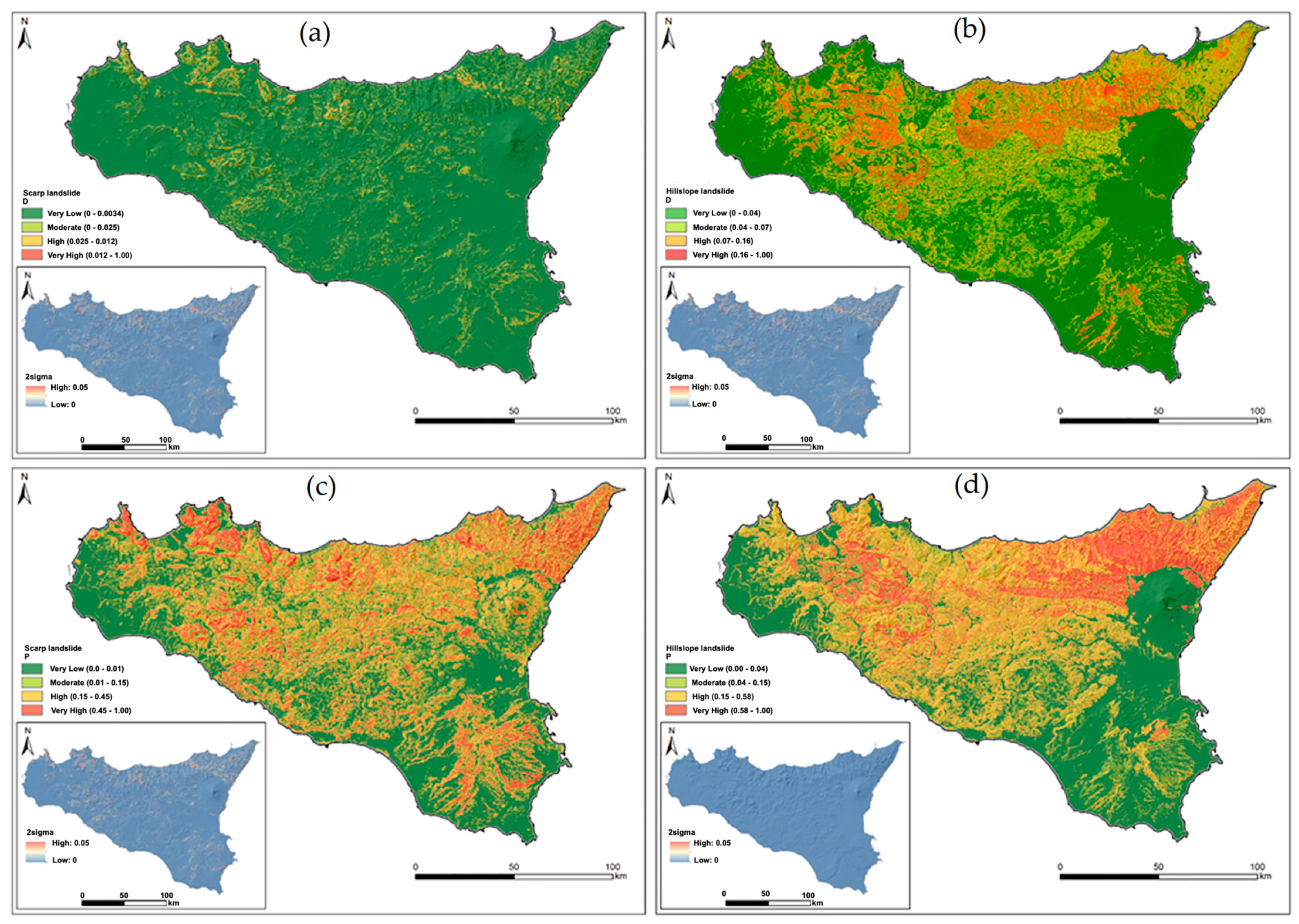
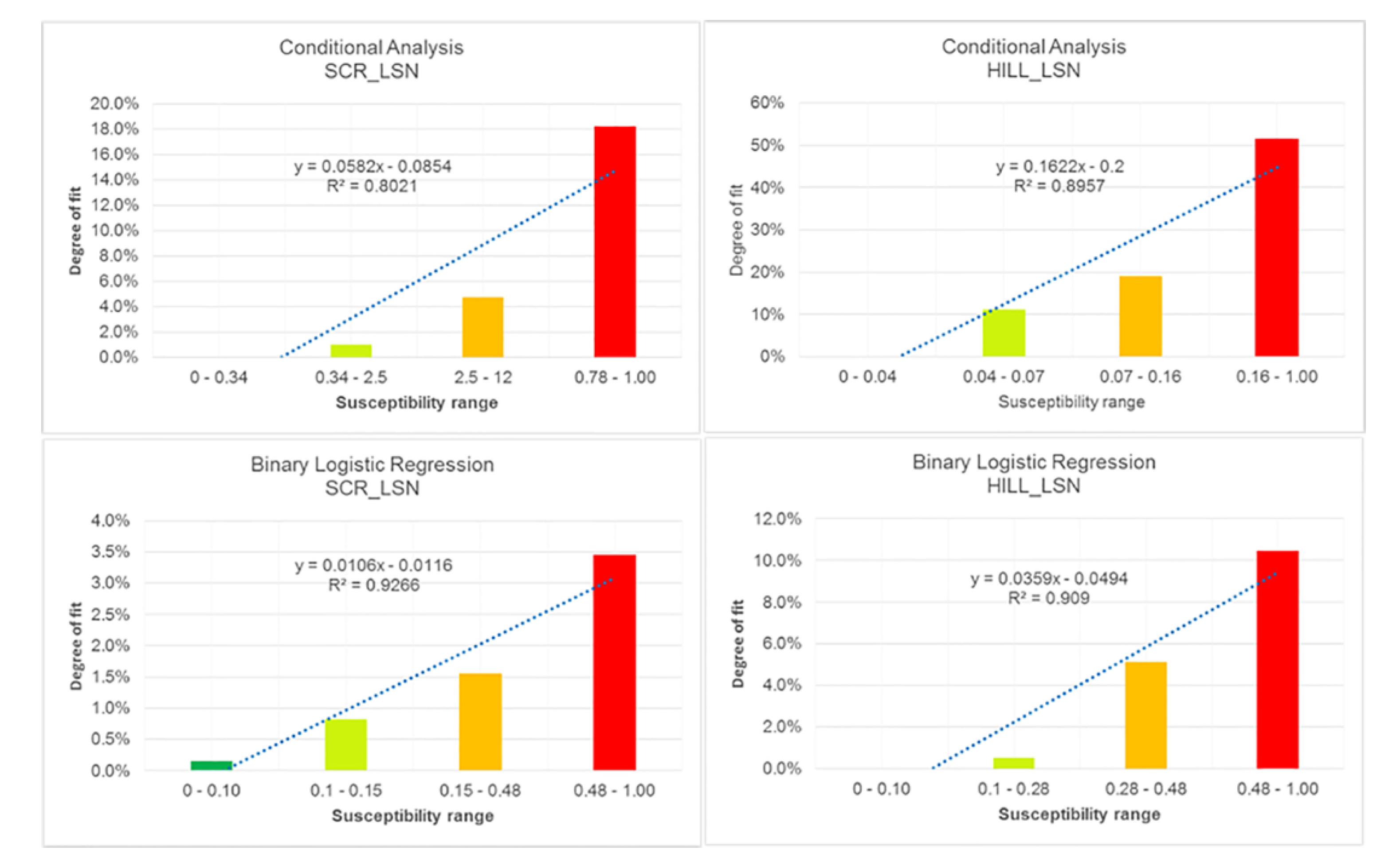
| (a) | CA | ||
| Landslide Tipology | |||
| SCR_LSN | HILL_LSN | ||
| Classes | Very Low | 0–0.34 | 0–0.04 |
| Moderate | 0.34–2.5 | 0.04–0.07 | |
| High | 2.5–12 | 0.07–0.16 | |
| Very High | 0.78–1.00 | 0.16–1.00 | |
| (b) | BLR | ||
| Landslide Tipology | |||
| SCR_LSN | HILL_LSN | ||
| Classes | Very Low | 0–0.10 | 0–0.10 |
| Moderate | 0.1–0.15 | 0.1–0.28 | |
| High | 0.15–0.48 | 0.28–0.48 | |
| Very High | 0.48–1.00 | 0.48–1.00 | |
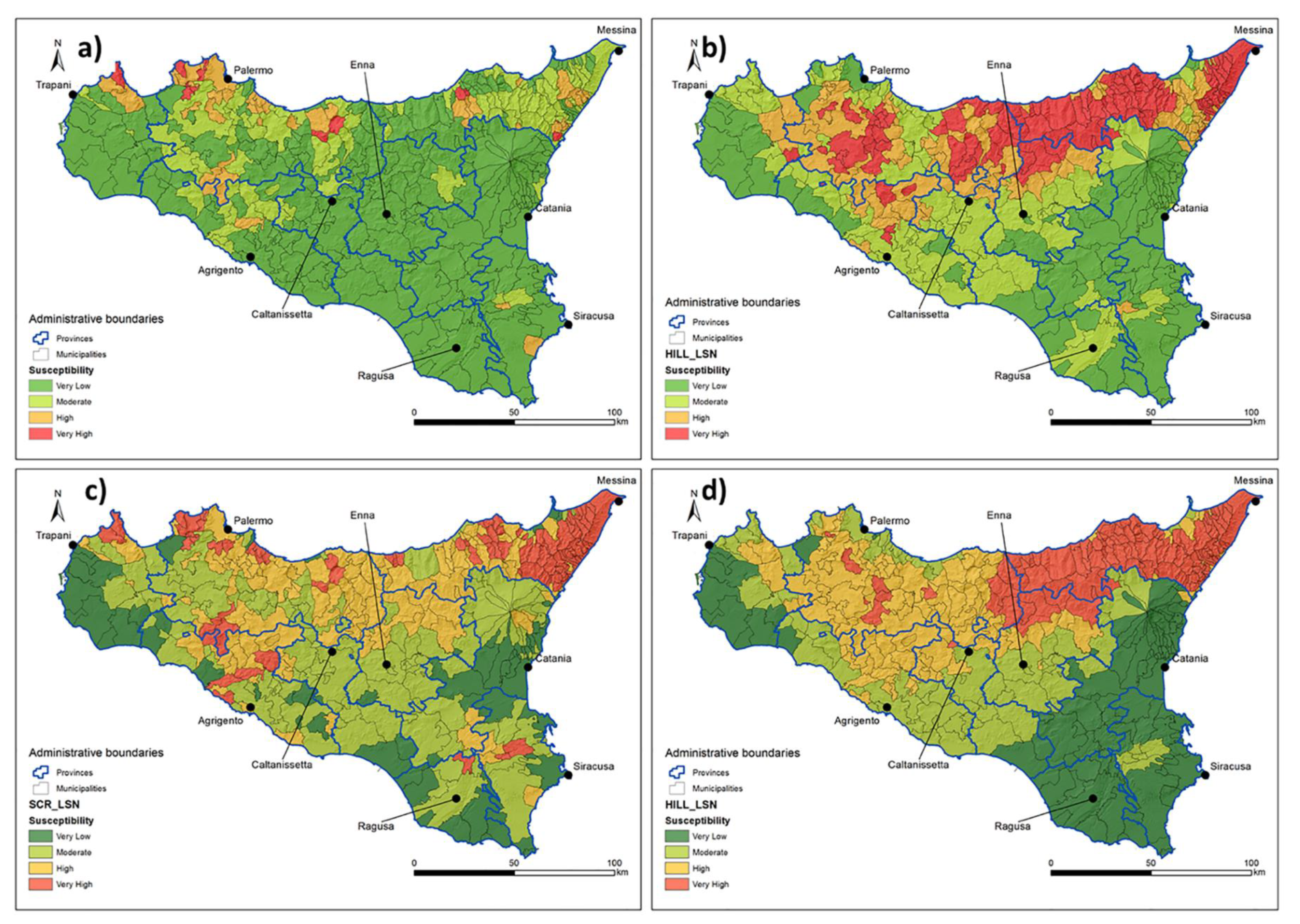
| (a) Munipality | Area (km2) | P | D | odd | km2 |
| SAN VITO LO CAPO | 3.6 | 4.42% | 1.98% | 2.44% | 3.91 |
| FRAZZANO’ | 1.2 | 5.90% | 3.02% | 2.88% | 1.46 |
| GIARDINELLO | 50.8 | 5.76% | 2.33% | 3.42% | 0.89 |
| ISNELLO | 6.9 | 6.76% | 3.70% | 3.05% | 0.82 |
| TORRETTA | 26.0 | 4.28% | 1.61% | 2.67% | 0.69 |
| SAN MARCO D’ALUNZIO | 12.8 | 5.85% | 2.58% | 3.27% | 0.23 |
| BORGETTO | 26.0 | 5.12% | 2.97% | 2.16% | 0.14 |
| CINISI | 33.0 | 4.81% | 2.57% | 2.24% | 0.14 |
| ISOLA DELLE FEMMINE | 60.2 | 10.70% | 7.04% | 3.66% | 0.13 |
| ROCCAFIORITA | 25.5 | 9.49% | 6.04% | 3.45% | 0.04 |
| (b) Munipality | Area (km2) | P | D | odd | km2 |
| FICARRA | 215.6 | 88.85% | 3.72% | 85.13% | 8.03 |
| SINAGRA | 70.0 | 93.26% | 9.34% | 83.91% | 6.54 |
| ALCARA LI FUSI | 31.1 | 91.98% | 16.74% | 75.24% | 5.21 |
| CASTELL’UMBERTO | 30.2 | 92.05% | 7.31% | 84.74% | 2.21 |
| SAN PIERO PATTI | 14.4 | 89.30% | 9.77% | 79.52% | 1.40 |
| MONTAGNAREALE | 11.4 | 89.73% | 11.07% | 78.66% | 1.26 |
| RACCUJA | 15.8 | 88.78% | 5.60% | 83.19% | 0.88 |
| UCRIA | 26.1 | 94.39% | 3.14% | 91.25% | 0.82 |
| SANT’ANGELO DI BROLO | 18.5 | 89.90% | 4.34% | 85.56% | 0.80 |
| TORTORICI | 23.9 | 89.21% | 2.76% | 86.46% | 0.66 |
© 2020 by the authors. Licensee MDPI, Basel, Switzerland. This article is an open access article distributed under the terms and conditions of the Creative Commons Attribution (CC BY) license (http://creativecommons.org/licenses/by/4.0/).
Share and Cite
Costanzo, D.; Irigaray, C. Comparing Forward Conditional Analysis and Forward Logistic Regression Methods in a Landslide Susceptibility Assessment: A Case Study in Sicily. Hydrology 2020, 7, 37. https://doi.org/10.3390/hydrology7030037
Costanzo D, Irigaray C. Comparing Forward Conditional Analysis and Forward Logistic Regression Methods in a Landslide Susceptibility Assessment: A Case Study in Sicily. Hydrology. 2020; 7(3):37. https://doi.org/10.3390/hydrology7030037
Chicago/Turabian StyleCostanzo, Dario, and Clemente Irigaray. 2020. "Comparing Forward Conditional Analysis and Forward Logistic Regression Methods in a Landslide Susceptibility Assessment: A Case Study in Sicily" Hydrology 7, no. 3: 37. https://doi.org/10.3390/hydrology7030037
APA StyleCostanzo, D., & Irigaray, C. (2020). Comparing Forward Conditional Analysis and Forward Logistic Regression Methods in a Landslide Susceptibility Assessment: A Case Study in Sicily. Hydrology, 7(3), 37. https://doi.org/10.3390/hydrology7030037