On the Ability of LIDAR Snow Depth Measurements to Determine or Evaluate the HRU Discretization in a Land Surface Model


Abstract
1. Introduction
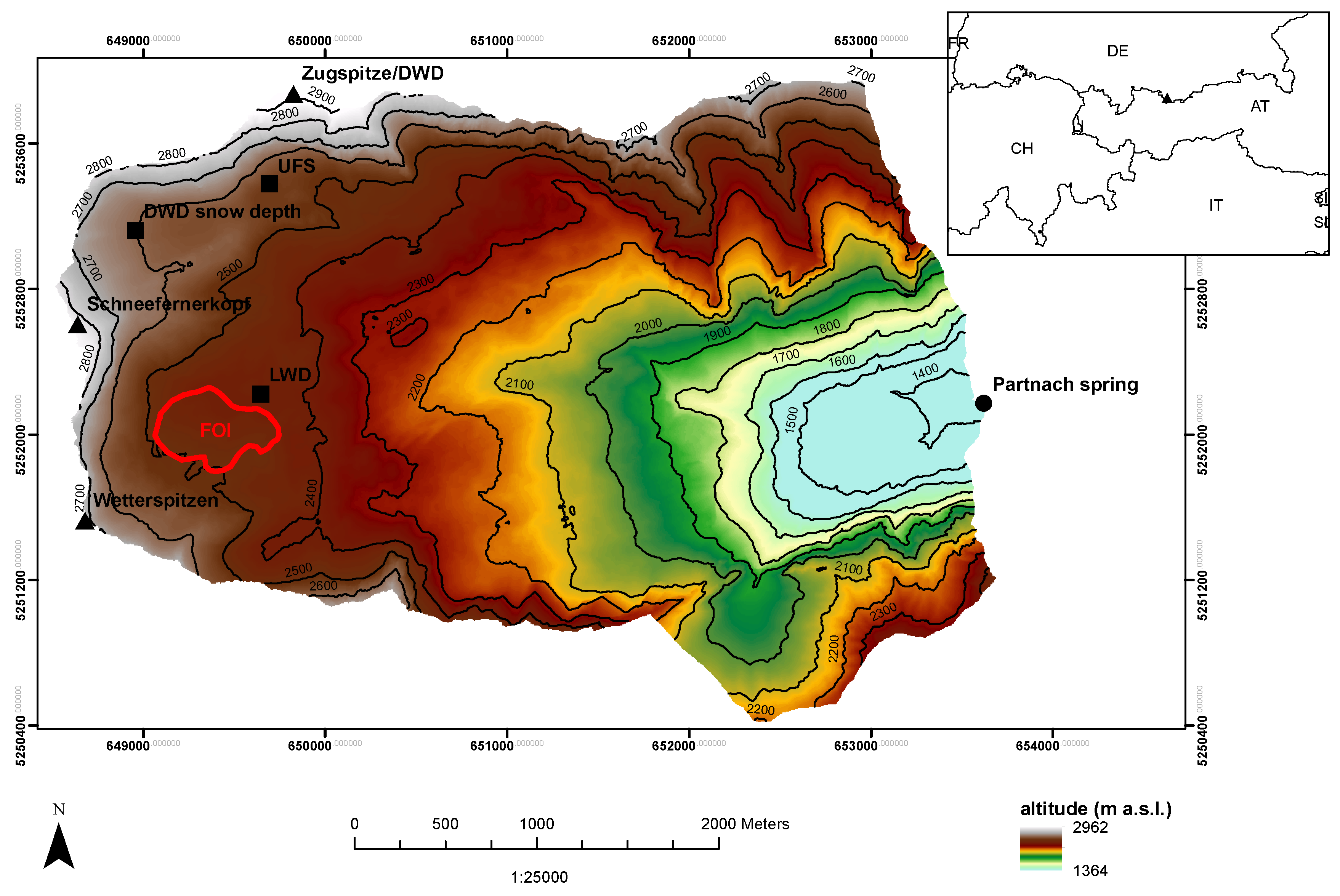
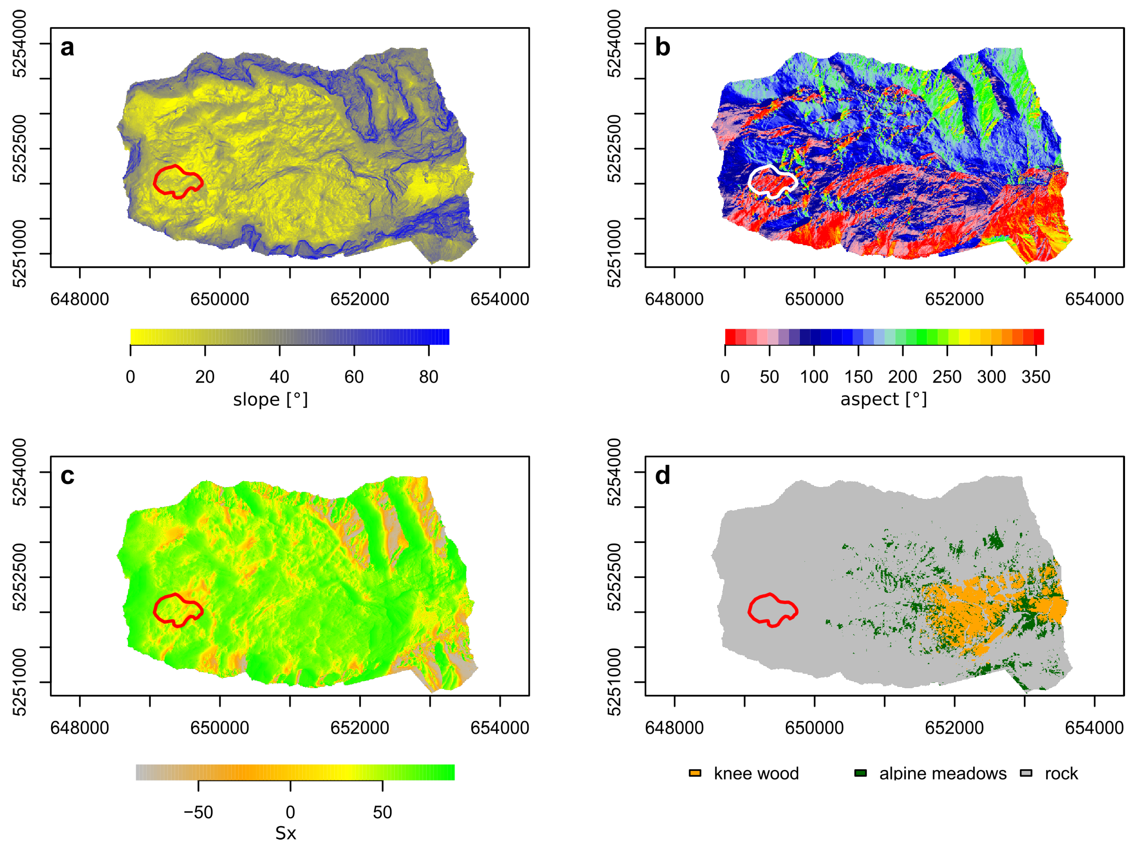
2. Study Area
3. Materials and Methods
3.1. Hydrological Modelling
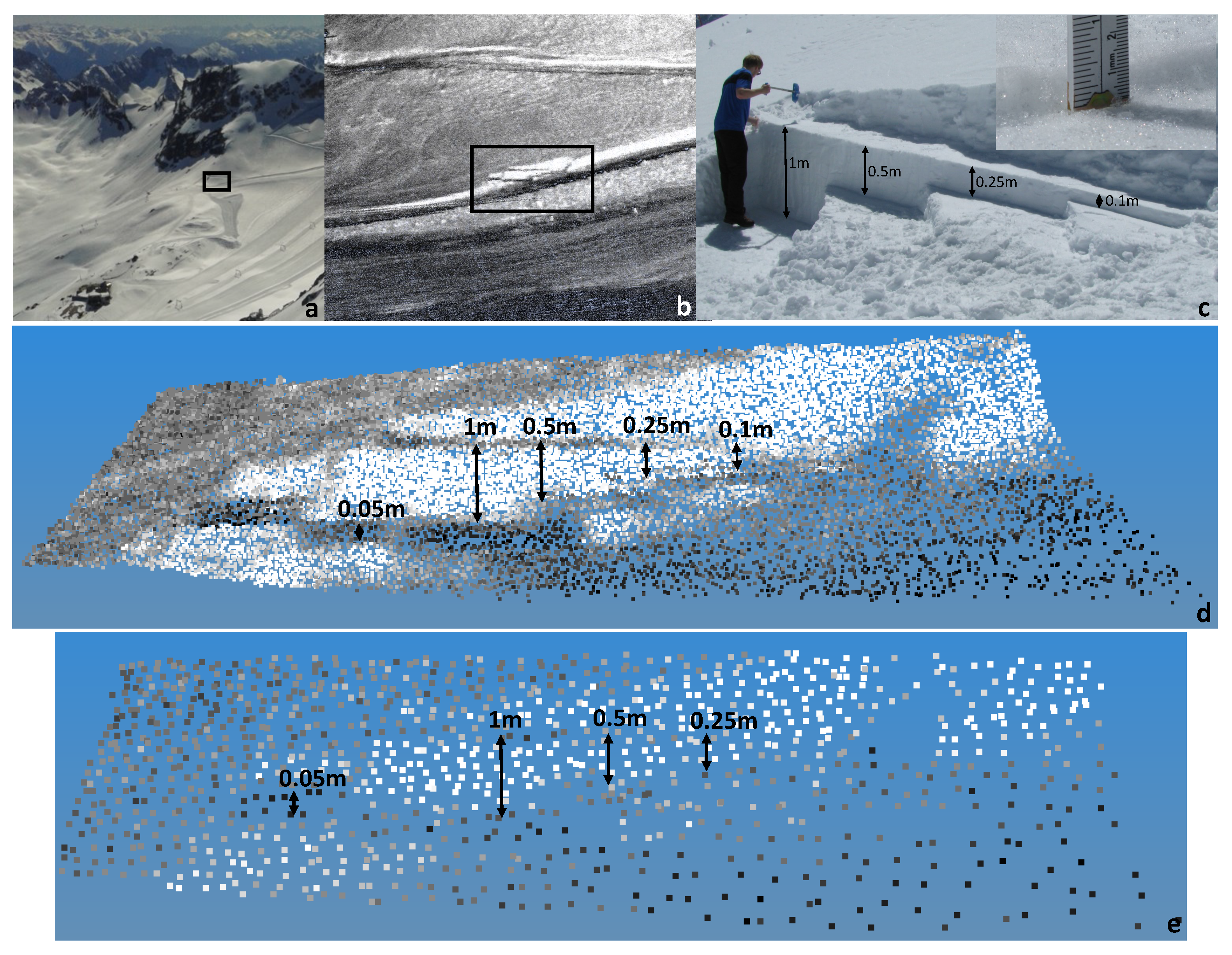
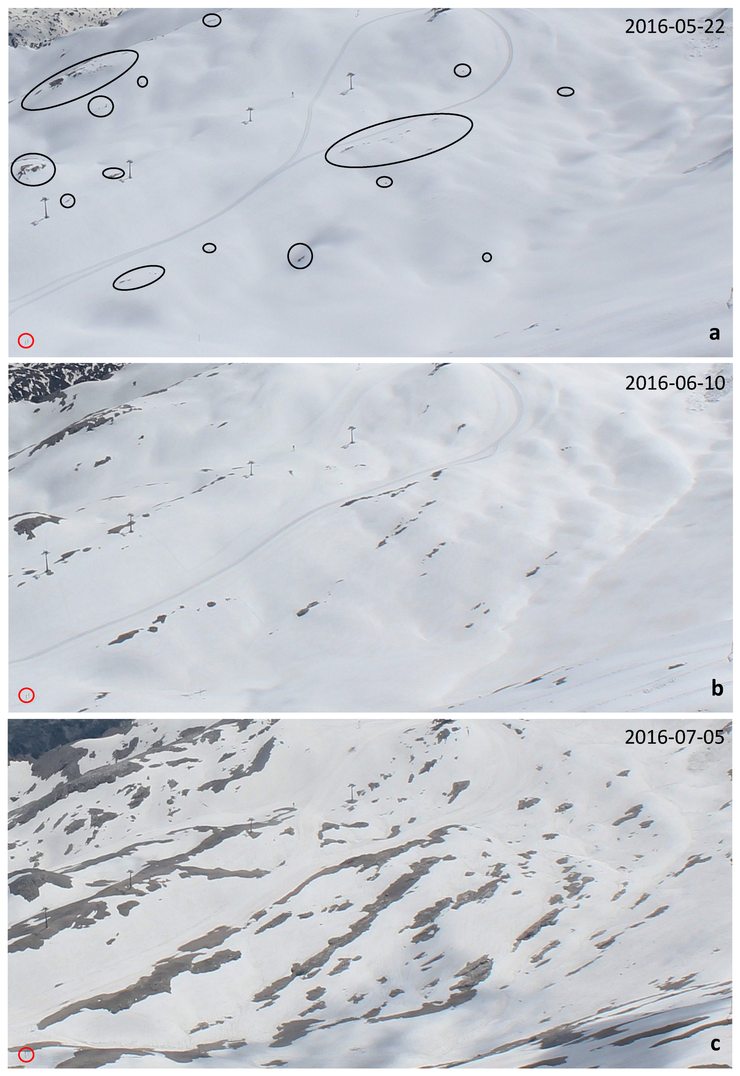
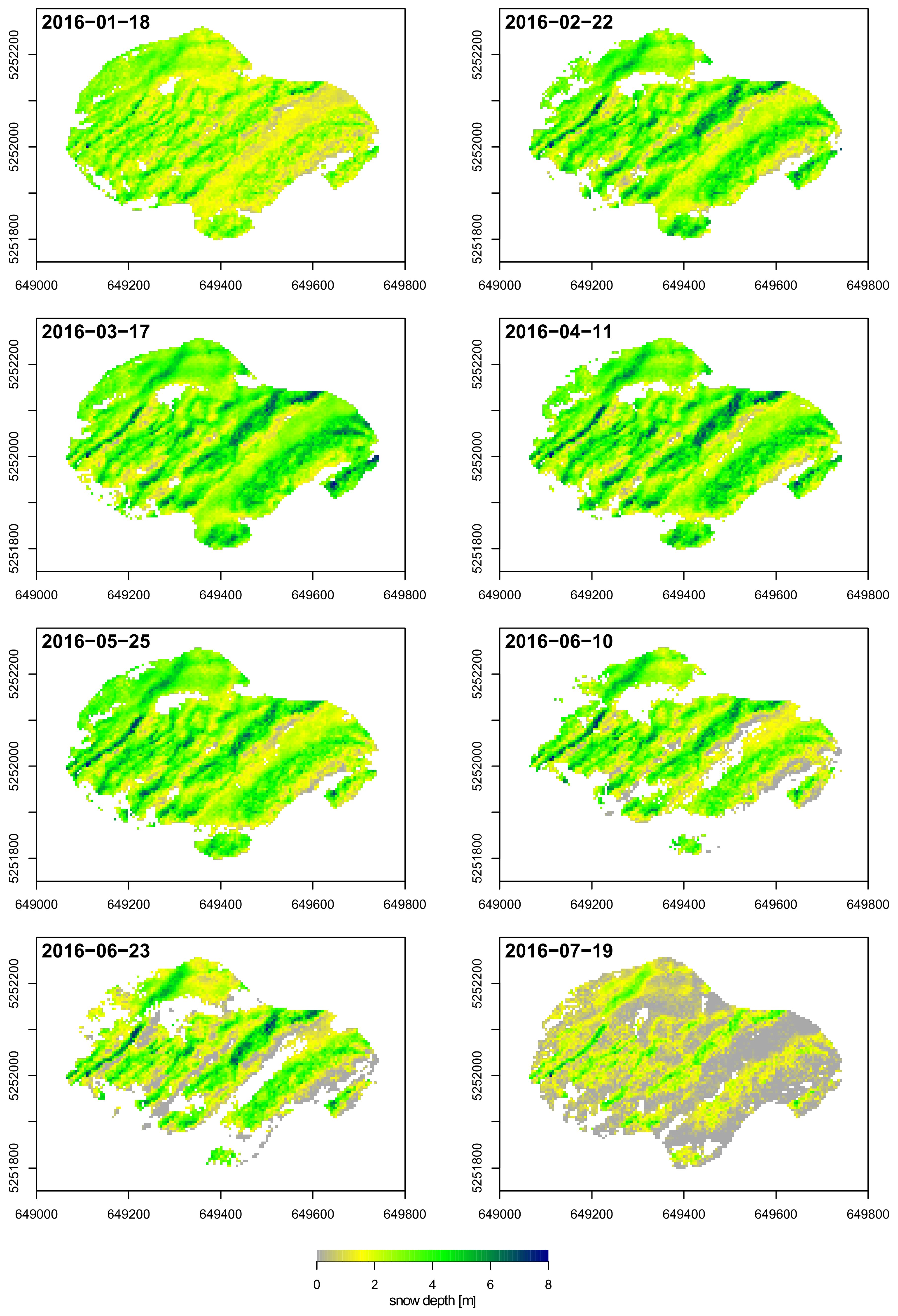
3.2. LIDAR Snow Depth Measurements and Its Analysis
3.3. Cluster Analysis
4. Results and Discussion
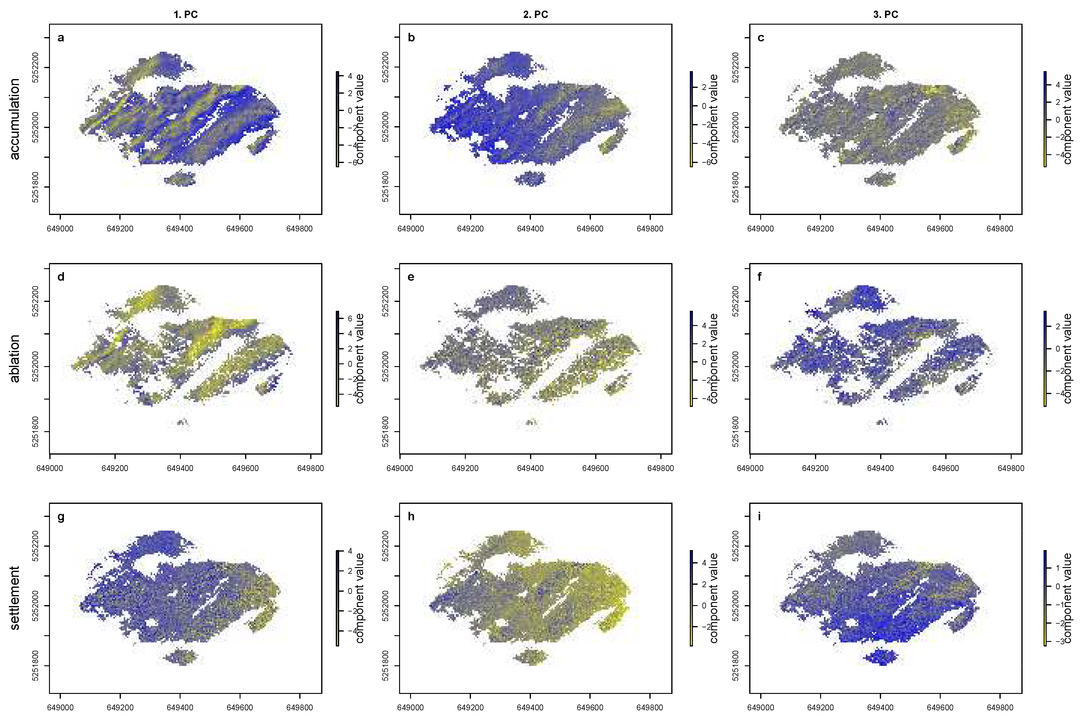
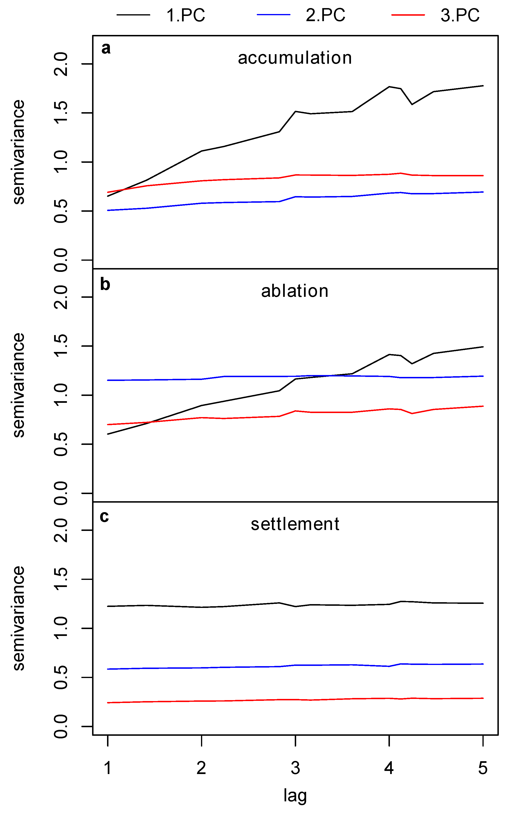
4.1. PCA Derived Patterns in Snow Cover
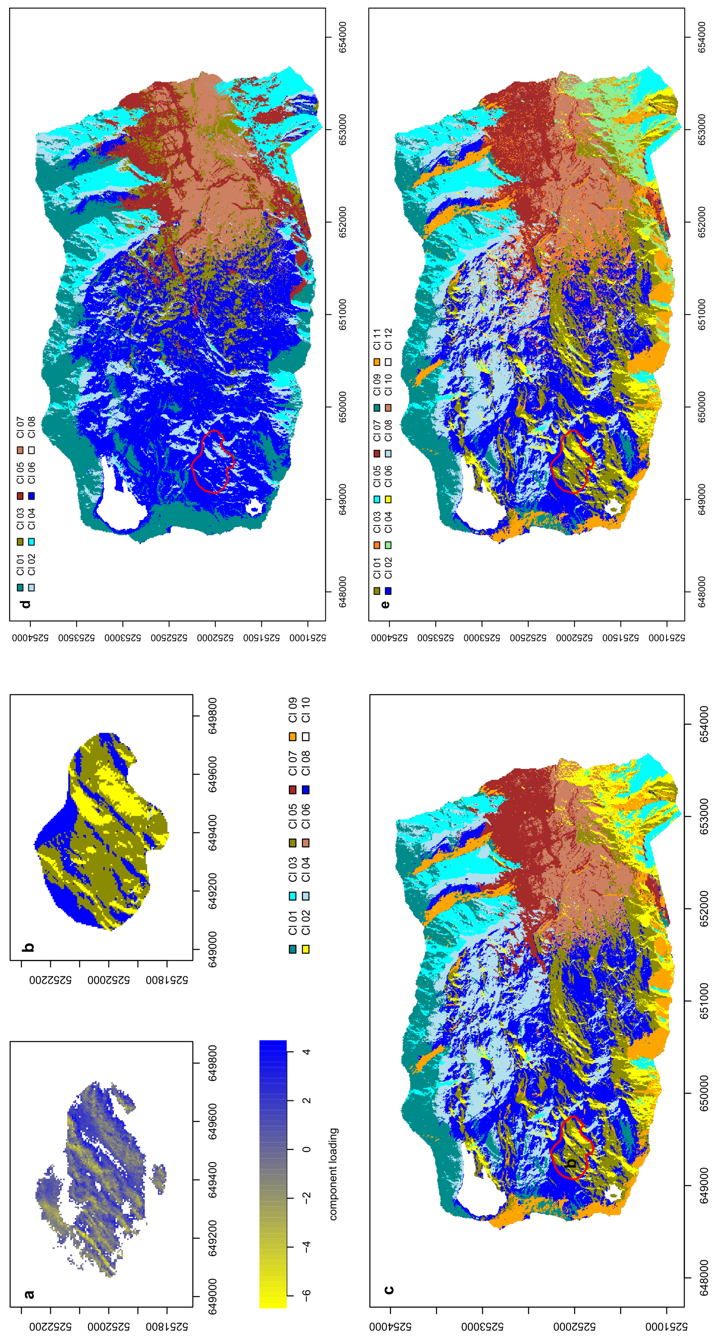
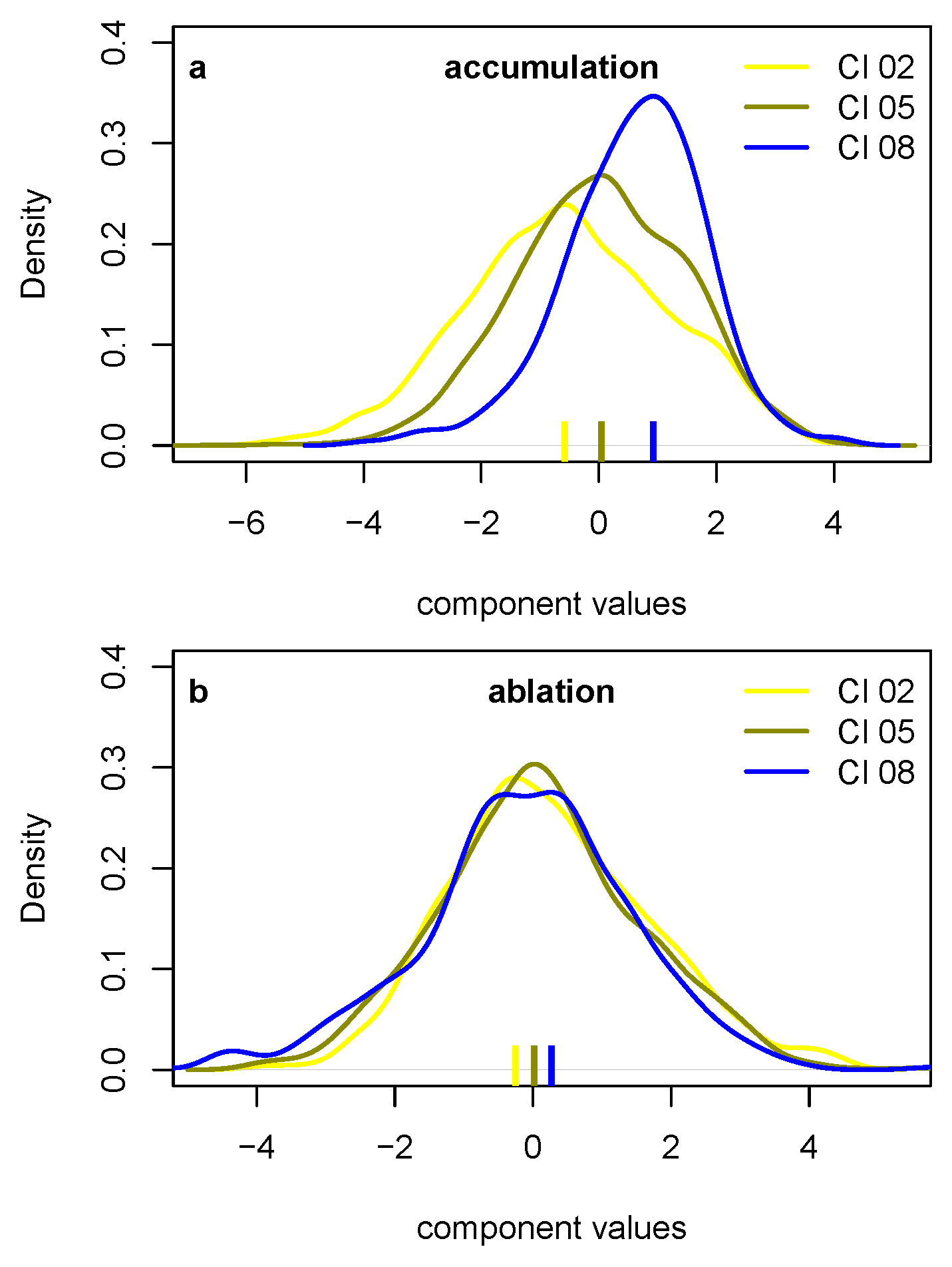
4.2. Cluster Analysis Results and HRU Delineation
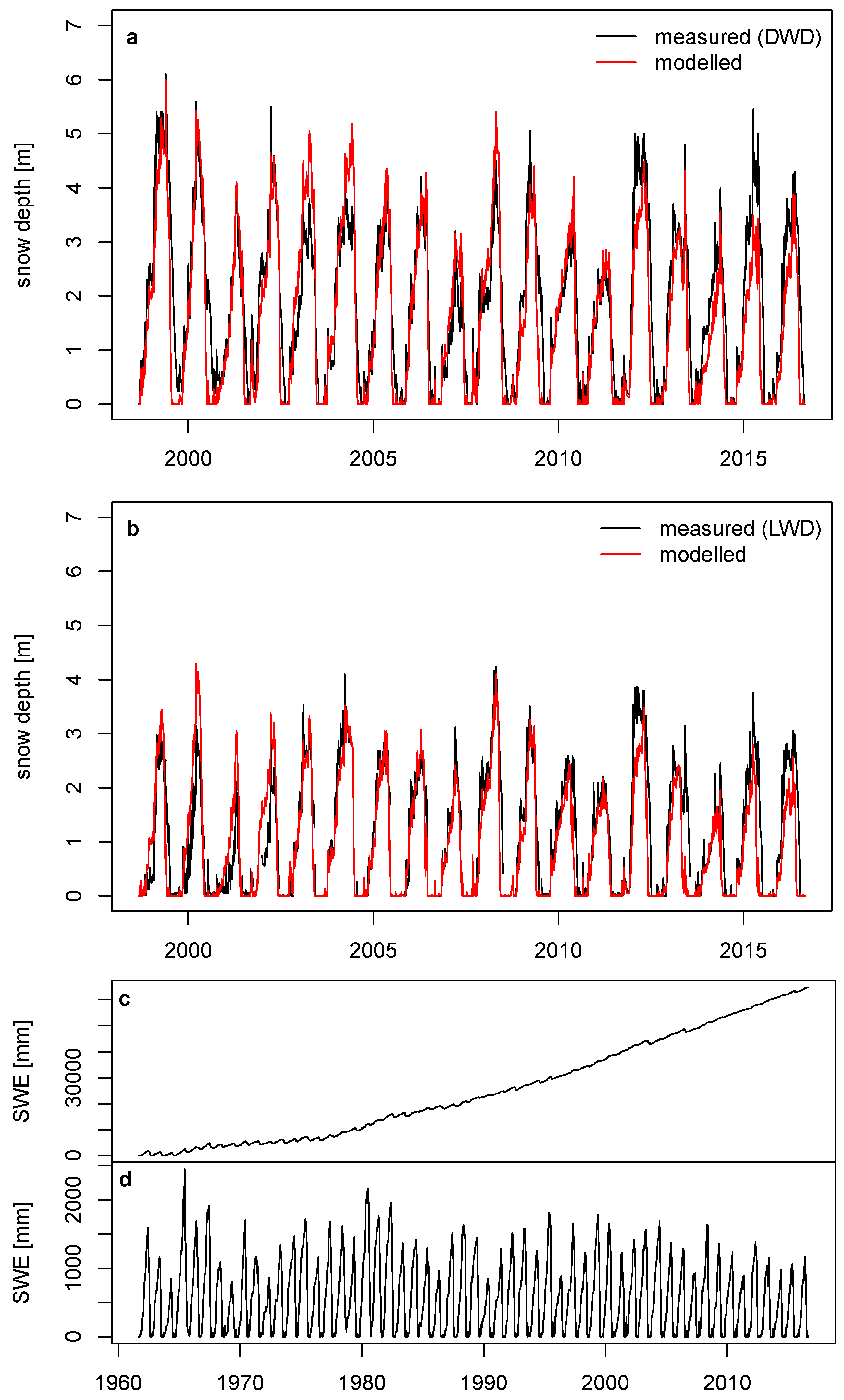
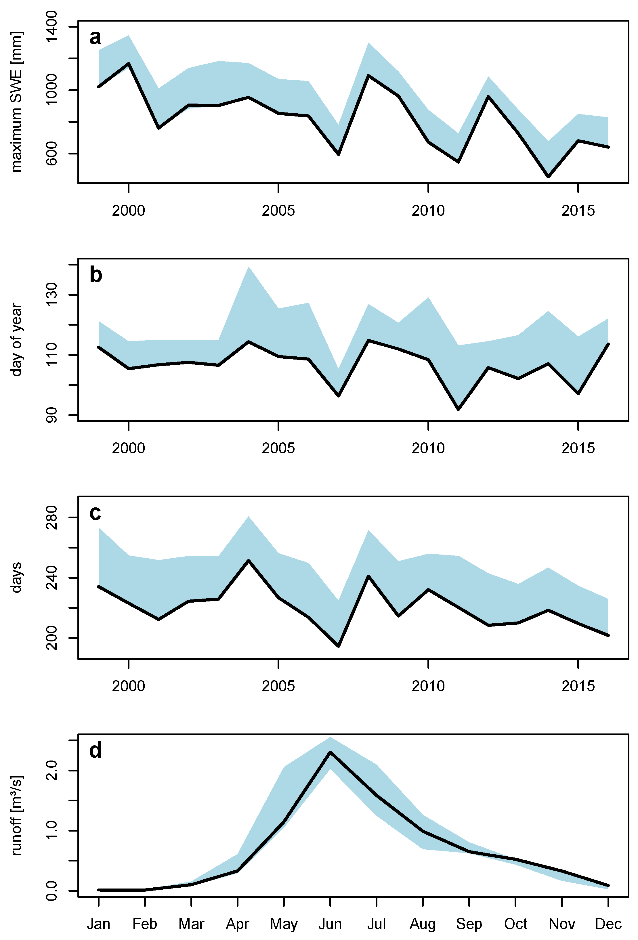
4.3. Evaluation of HRU Schemes with Station Measurement Data and Effects on Snow Parameters and Runoff
5. Conclusions and Outlook
Author Contributions
Funding
Acknowledgments
Conflicts of Interest
Abbreviations
| SWE | snow water equivalent |
| MSWE | maximum snow water equivalent |
| DoMSWE | day of maximum snow water equivalent |
| NSE | Nash-Sucliffe efficiency |
| CRHM | Cold Regions Hydrological Model |
| HRU | hydrological response unit |
| DWD | Deutscher Wetterdienst (Germen Weather Service) |
| LWD | Lawinenwarndienst Bayern (Bavarian Avalanche Service) |
| RCZ | Research Catchment Zugspitze |
| PCA | principle component analysis |
| FOI | field of interest |
| DEM | digital elevation model |
| Sx | wind sheltering index |
| LIDAR | light detection and ranging |
Appendix A

References
- Grünewald, T.; Schirmer, M.; Mott, R.; Lehning, M. Spatial and temporal variability of snow depth and ablation rates in a small mountain catchment. Cryosphere 2010, 4, 215–225. [Google Scholar] [CrossRef]
- Fatichi, S.; Vivoni, E.R.; Ogden, F.L.; Ivanov, V.Y.; Mirus, B.; Gochis, D.; Downer, C.W.; Camporese, M.; Davison, J.H.; Ebel, B.; et al. An overview of current applications, challenges, and future trends in distributed process-based models in hydrology. J. Hydrol. 2016, 537, 45–60. [Google Scholar] [CrossRef]
- Klemeš, V. The modelling of mountain hydrology: The ultimate challenge. In Hydrology of Mountain Areas; IAHS Publisher: Wallingford, UK, 1990; pp. 29–43. [Google Scholar]
- Dehotin, J.; Braud, I. Which spatial discretization for distributed hydrological models? Proposition of a methodology and illustration for medium to large-scale catchments. Hydrol. Earth Syst. Sci. 2008, 12, 769–796. [Google Scholar] [CrossRef]
- Schulla, J. Model Description WaSiM.Zürich Hydrology Software Consulting. Available online: http://www.wasim.ch/en/products/wasim_description.htm (accessed on 9 February 2020).
- Lehning, M.; Völksch, I.; Gustafsson, D.; Nguyen, T.A.; Stähli, M.; Zappa, M. ALPINE3D: A detailed model of mountain surface processes and its application to snow hydrology. Hydrol. Process. 2006, 20, 2111–2128. [Google Scholar] [CrossRef]
- Samaniego, L.; Kumar, R.; Jackisch, C. Predictions in a data-sparse region using a regionalized grid-based hydrologic model driven by remotely sensed data. Hydrol. Res. 2011, 42, 338–355. [Google Scholar] [CrossRef]
- Flügel, W. Delineating hydrological response units by geographical information system analyses for regional hydrological modelling using PRMS/MMS in the drainage basin of the River Bröl, Germany. Hydrol. Process. 1995, 1995, 423–436. [Google Scholar] [CrossRef]
- Leavesley, G.H.; Lichty, R.W.; Troutman, B.M.; Saindon, L.G. Precipitation-Runoff Modeling System; User’s Manual; U.S. Geological Survey, Water Resources Division: Reston, VA, USA, 1983. [Google Scholar] [CrossRef]
- Neitsch, S.L.; Arnold, J.G.; Kiniry, J.R.; Williams, J.R. Soil and Water Assessment Tool, SWAT 2009. Theoretical Documentation. Available online: http://swat.tamu.edu/media/99192/swat2009-theory.pdf (accessed on 9 February 2020).
- Pomeroy, J.W.; Gray, D.M.; Brown, T.; Hedstrom, N.R.; Quinton, W.L.; Granger, R.J.; Carey, S.K. The cold regions hydrological model: A platform for basing process representation and model structure on physical evidence. Hydrol. Process. 2007, 21, 2650–2667. [Google Scholar] [CrossRef]
- Zehe, E.; Ehret, U.; Pfister, L.; Blume, T.; Schröder, B.; Westhoff, M.; Jackisch, C.; Schymanski, S.J.; Weiler, M.; Schulz, K.; et al. HESS Opinions: From response units to functional units: A thermodynamic reinterpretation of the HRU concept to link spatial organization and functioning of intermediate scale catchments. Hydrol. Earth Syst. Sci. 2014, 18, 4635–4655. [Google Scholar] [CrossRef]
- Savvidou, E.; Efstratiadis, A.; Koussis, A.D.; Koukouvinos, A.; Skarlatos, D. A curve number approach to formulate hydrological response units within distributed hydrological modelling. Hydrol. Earth Syst. Sci. Discuss. 2016, 12, 1–34. [Google Scholar] [CrossRef]
- Savvidou, E.; Efstratiadis, A.; Koussis, A.; Koukouvinos, A.; Skarlatos, D. The Curve Number Concept as a Driver for Delineating Hydrological Response Units. Water 2018, 10, 194. [Google Scholar] [CrossRef]
- Balk, B.; Elder, K. Combining binary decision tree and geostatistical methods to estimate snow distribution in a mountain watershed. Water Resour. Res. 2000, 36, 13–26. [Google Scholar] [CrossRef]
- Liston, G.E. Representing Subgrid Snow Cover Heterogeneities in Regional and Global Models. J. Clim. 2004, 17, 1381–1397. [Google Scholar] [CrossRef]
- Winstral, A.; Elder, K.; Davis, R.E. Spatial Snow Modeling of Wind-Redistributed Snow Using Terrain-Based Parameters. J. Hydrometeorol. 2002, 3, 524–538. [Google Scholar] [CrossRef]
- Winstral, A.; Marks, D. Long-term snow distribution observations in a mountain catchment: Assessing variability, time stability, and the representativeness of an index site. Water Resour. Res. 2014, 50, 293–305. [Google Scholar] [CrossRef]
- Gampe, D.; Ludwig, R. Evaluation of Gridded Precipitation Data Products for Hydrological Applications in Complex Topography. Hydrology 2017, 4, 53. [Google Scholar] [CrossRef]
- Burlando, P.; Pellicciotti, F.; Strasser, U. Modelling Mountainous Water Systems Between Learning and Speculating Looking for Challenges. Hydrol. Res. 2002, 33, 47–74. [Google Scholar] [CrossRef]
- DeBeer, C.M.; Pomeroy, J.W. Simulation of the snowmelt runoff contributing area in a small alpine basin. Hydrol. Earth Syst. Sc. 2010, 14, 1205–1219. [Google Scholar] [CrossRef]
- DeBeer, C.M.; Pomeroy, J.W. Influence of snowpack and melt energy heterogeneity on snow cover depletion and snowmelt runoff simulation in a cold mountain environment. J. Hydrol. 2017, 553, 199–213. [Google Scholar] [CrossRef]
- Strasser, U.; Kunstmann, H. Tackling complexity in modelling mountain hydrology: Where do we stand, where do we go? In Cold and Mountain Region Hydrological Systems Under Climate Change: Towards Improved Projections; IAHS Publisher: Wallingford, UK, 2013; pp. 3–12. [Google Scholar]
- Prasch, M.; Mauser, W.; Weber, M. Quantifying present and future glacier melt-water contribution to runoff in a central Himalayan river basin. Cryosphere 2013, 7, 889–904. [Google Scholar] [CrossRef]
- Stahl, K.; Weiler, M.; Kohn, I.; Freudiger, D.; Seibert, J.; Vis, M.; Gerlinger, K.; Böhm, M. The Snow and Glacier Melt Components of Streamflow of the River Rhine and Its Tributaries Considering the Influence of Climate Change; Vol. Nr. 25, Report KHR. 1; Internationale Kommission für die Hydrologie des Rheingebietes (KHR/CHR): Lelystad, The Netherlands, 2016. [Google Scholar]
- Verbunt, M.; Gurtz, J.; Jasper, K.; Lang, H.; Warmerdam, P.; Zappa, M. The hydrological role of snow and glaciers in alpine river basins and their distributed modeling. J. Hydrol. 2003, 282, 36–55. [Google Scholar] [CrossRef]
- Engelhardt, M.; Schuler, T.V.; Andreassen, L.M. Contribution of snow and glacier melt to discharge for highly glacierised catchments in Norway. Hydrol. Earth Syst. Sci. 2014, 18, 511–523. [Google Scholar] [CrossRef]
- Wulf, H.; Bookhagen, B.; Scherler, D. Differentiating between rain, snow, and glacier contributions to river discharge in the western Himalaya using remote-sensing data and distributed hydrological modeling. Adv. Water Resour. 2015, 2015. [Google Scholar] [CrossRef]
- Currier, W.R.; Pflug, J.; Mazzotti, G.; Jonas, T.; Deems, J.S.; Bormann, K.J.; Painter, T.H.; Hiemstra, C.A.; Gelvin, A.; Uhlmann, Z.; et al. Comparing Aerial Lidar Observations With Terrestrial Lidar and Snow–Probe Transects From NASA’s 2017 SnowEx Campaign. Water Resour. Res. 2019, 55, 6285–6294. [Google Scholar] [CrossRef]
- Deems, J.S.; Painter, T.H.; Finnegan, D.C. Lidar measurement of snow depth: A review. J. Glaciol. 2013, 59, 467–479. [Google Scholar] [CrossRef]
- Egli, L.; Jonas, T.; Grünewald, T.; Schirmer, M.; Burlando, P. Dynamics of snow ablation in a small Alpine catchment observed by repeated terrestrial laser scans. Hydrol. Process. 2012, 26, 1574–1585. [Google Scholar] [CrossRef]
- Prokop, A. Assessing the applicability of terrestrial laser scanning for spatial snow depth measurements. Cold Reg. Sci. Technol. 2008, 54, 155–163. [Google Scholar] [CrossRef]
- Schön, P.; Prokop, A.; Vionnet, V.; Guyomarc’h, G.; Naaim-Bouvet, F.; Heiser, M. Improving a terrain-based parameter for the assessment of snow depths with TLS data in the Col du Lac Blanc area. Cold Reg. Sci. Technol. 2015, 114, 15–26. [Google Scholar] [CrossRef]
- de Almeida, T.I.R.; Penatti, N.C.; Ferreira, L.G.; Arantes, A.E.; do Amaral, C.H. Principal component analysis applied to a time series of MODIS images: The spatio-temporal variability of the Pantanal wetland, Brazil. Wetl. Ecol. Manag. 2015, 23, 737–748. [Google Scholar] [CrossRef]
- Coppin, P.; Jonckheere, I.; Nackaerts, K.; Muys, B.; Lambin, E. Digitalchange detection methods in ecosystem monitoring: A review. Int. J. Remote Sens. 2004, 25, 1565–1596. [Google Scholar] [CrossRef]
- Müller, B.; Bernhardt, M.; Schulz, K. Identification of catchment functional units by time series of thermal remote sensing images. Hydrol. Earth Syst. Sci. 2014, 18, 5345–5359. [Google Scholar] [CrossRef]
- Weber, M.; Bernhardt, M.; Pomeroy, J.W.; Fang, X.; Härer, S.; Schulz, K. Description of current and future snow processes in a small basin in the Bavarian Alps. Environ. Earth Sci. 2016, 75, 962. [Google Scholar] [CrossRef]
- Friedmann, A.; Korch, O. Die Vegetation des Zugspitzplatts (Wettersteingebirge, Bayerische Alpen): Aktueller Zustand und Dynamik. Berichte der Reinhold-Tüxen-Gesellschaft 2010, 22, 114–128. [Google Scholar]
- Rappl, A.; Wetzel, K.F.; Büttner, G.; Scholz, M. Tracerhydrolgische Untersuchungen am Partnach-Ursprung: Dye tracer investigation at the Partnach Spring (German Alps). Hydrol. Wasserbewirtsch. 2010, 54, 220–230. [Google Scholar]
- Wetzel, K.F. On the Hydrology of the Partnach Area in the Wetterstein Mountains (Bavarian Alps). Erdkunde 2004, 58, 172–186. [Google Scholar] [CrossRef]
- Dornes, P.F.; Pomeroy, J.W.; Pietroniro, A.; Carey, S.K.; Quinton, W.L. Influence of landscape aggregation in modelling snow-cover ablation and snowmelt runoff in a sub-arctic mountainous environment. Hydrolog. Sci. J. 2008, 53, 725–740. [Google Scholar] [CrossRef]
- Ellis, C.R.; Pomeroy, J.W.; Brown, T.; MacDonald, J. Simulations of snow accumulation and melt in needleleaf forest environments. Hydrol. Earth Syst. Sci. 2010, 14, 925–940. [Google Scholar] [CrossRef]
- Essery, R.; Rutter, N.; Pomeroy, J.W.; Baxter, R.; Stähli, M.; Gustafsson, D.; Barr, A.; Bartlett, P.; Elder, K. SNOWMIP2: An Evaluation of Forest Snow Process Simulations. Am. Meteorol. Soc. 2009, 90, 1120–1135. [Google Scholar] [CrossRef]
- Fang, X.; Pomeroy, J.W. Impact of antecedent conditions on simulations of a flood in a mountain headwater basin. Hydrol. Process. 2016, 30, 2754–2772. [Google Scholar] [CrossRef]
- López-Moreno, J.I.; Pomeroy, J.W.; Revuelto, J.; Vicente-Serrano, S.M. Response of snow processes to climate change: Spatial variability in a small basin in the Spanish Pyrenees. Hydrol. Process. 2013, 27, 2637–2650. [Google Scholar] [CrossRef]
- Pomeroy, J.W.; Gray, D.M.; Landine, P.G. The Prairie Blowing Snow Model: Characteristics, validation, operation. J. Hydrol. 1993, 144, 165–192. [Google Scholar] [CrossRef]
- Pomeroy, J.W.; Stewart, R.E.; Whitfield, P.H. The 2013 flood event in the South Saskatchewan and Elk River basins: Causes, assessment and damages. Can. Water Resour. J. / Rev. Can. Des Ressour. Hydr. 2016, 41, 105–117. [Google Scholar] [CrossRef]
- Liston, G.E.; Elder, K. A Meteorological Distribution System for High-Resolution Terrestrial Modeling (MicroMet). J. Hydrometeorol. 2006, 7, 217–234. [Google Scholar] [CrossRef]
- Jennings, K.S.; Winchell, T.S.; Livneh, B.; Molotch, N.P. Spatial variation of the rain-snow temperature threshold across the Northern Hemisphere. Nat. Commun. 2018, 9, 1148. [Google Scholar] [CrossRef] [PubMed]
- WMO. Technical Regulations: Basic Documents No. 2: Volume I—General Meteorological Standards and Recommended Practices, 2010 ed.; World Meteorological Organization: Geneva, Switzerland, 2011. [Google Scholar]
- Grossi, G.; Lendvai, A.; Peretti, G.; Ranzi, R. Snow Precipitation Measured by Gauges: Systematic Error Estimation and Data Series Correction in the Central Italian Alps. Water 2017, 9, 461. [Google Scholar] [CrossRef]
- MacDonald, M.K.; Pomeroy, J.W.; Pietroniro, A. Hydrological response unit-based blowing snow modelling over an alpine ridge. Hydrol. Earth Syst. Sci. 2010, 2010, 1167–1208. [Google Scholar] [CrossRef]
- Marks, D.; Domingo, J.; Susong, D.; Link, T.; Garen, D. A spatially distributed energy balance snowmelt model for application in mountain basins. Hydrol. Process. 1999, 13, 1935–1959. [Google Scholar]
- Garnier, B.J.; Ohmura, A. The evaluation of surface variations in solar radiation income. Sol. Energy 1970, 13, 21–34. [Google Scholar] [CrossRef]
- Essery, R.; Etchevers, P. Parameter sensitivity in simulations of snowmelt. J. Geophys. Res. 2004, 109. [Google Scholar] [CrossRef]
- Mott, R.; Egli, L.; Grünewald, T.; Dawes, N.; Manes, C.; Bavay, M.; Lehning, M. Micrometeorological processes driving snow ablation in an Alpine catchment. Cryosphere 2011, 5, 1083–1098. [Google Scholar] [CrossRef]
- Campanella, M.; Rossi, G.; Ruggiero, G. JRC 3D Reconstructor User Manual 2014: For An Easy Learning of JRC 3D Reconstructor Tools. Available online: www.gexcel.homeip.net/Reconstructor/R_Manual/R_ManualEN.pdf (accessed on 9 February 2020).
- Crósta, A.P.; de Souza Filho, C.R.; Azevedo, F.; Brodie, C. Targeting key alteration minerals in epithermal deposits in Patagonia, Argentina, using ASTER imagery and principal component analysis. Int. J. Remote Sens. 2003, 24, 4233–4240. [Google Scholar] [CrossRef]
- Richards, J.A. Remote Sensing Digital Image Analysis; Springer: Berlin/Heidelberg, Germany, 2013. [Google Scholar] [CrossRef]
- Rao, A.R.; Srinivas, V.V. Regionalization of watersheds by fuzzy cluster analysis. J. Hydrol. 2006, 318, 57–79. [Google Scholar] [CrossRef]
- Rao, A.R.; Srinivas, V.V. Regionalization of watersheds by hybrid-cluster analysis. J. Hydrol. 2006, 318, 37–56. [Google Scholar] [CrossRef]
- Sawicz, K.; Wagener, T.; Sivapalan, M.; Troch, P.A.; Carrillo, G. Catchment classification: Empirical analysis of hydrologic similarity based on catchment function in the eastern USA. Hydrol. Earth Syst. Sci. 2011, 15, 2895–2911. [Google Scholar] [CrossRef]
- Li, Q.; Li, Z.; Zhu, Y.; Deng, Y.; Zhang, K.; Yao, C. Hydrological regionalisation based on available hydrological information for runoff prediction at catchment scale. Proc. Int. Assoc. Hydrol. Sci. 2018, 379, 13–19. [Google Scholar] [CrossRef]
- Nied, M.; Hundecha, Y.; Merz, B. Flood-initiating catchment conditions: A spatio-temporal analysis of large-scale soil moisture patterns in the Elbe River basin. Hydrol. Earth Syst. Sci. 2013, 17, 1401–1414. [Google Scholar] [CrossRef]
- Dadic, R.; Mott, R.; Lehning, M.; Burlando, P. Wind influence on snow depth distribution and accumulation over glaciers. Environ. Res. Lett. 2010, 115, 1064. [Google Scholar] [CrossRef]
- Huang, Z. Extensions to the k-Means Algorithm for Clustering Large Data Sets with Categorical Values. Data Min. Knowl. Discov. 1998, 2, 283–304. [Google Scholar] [CrossRef]
- MacQueen, J.B. Some methods for classification and analysis of multivariate observations. In Proceedings of the Fifth Berkeley Symposium on Mathematical Statistics and Probability; Le Cam, L.M., Neyman, J., Eds.; University of California Press: Berkeley, CA, USA, 1967. [Google Scholar]
- Schirmer, M.; Wirz, V.; Clifton, A.; Lehning, M. Persistence in intra-annual snow depth distribution: 1. Measurements and topographic control. Water Resour. Res. 2011, 47, 435. [Google Scholar] [CrossRef]
- Schirmer, M.; Lehning, M. Persistence in intra-annual snow depth distribution: 2. Fractal analysis of snow depth development. Water Resour. Res. 2011, 47, 2373. [Google Scholar] [CrossRef]
- Winstral, A.; Marks, D.; Gurney, R. Simulating wind-affected snow accumulations at catchment to basin scales. Adv. Water Resour. 2013, 55, 64–79. [Google Scholar] [CrossRef]
- Mott, R.; Scipión, D.; Schneebeli, M.; Dawes, N.; Berne, A.; Lehning, M. Orographic effects on snow deposition patterns in mountainous terrain. J. Geophys. Res. Atmos. 2014, 119, 1419–1439. [Google Scholar] [CrossRef]
- Ohmura, A. Physical Basis for the Temperature-Based Melt Index Method. J. Appl. Meteorol. 2001, 40, 753–761. [Google Scholar] [CrossRef]
- Marsh, P.; Pomeroy, J.W.; Neumann, N. Sensible heat flux and local advection over a heterogeneous landscape at an Arctic tundra site during snowmelt. Ann. Glaciol. 1997, 25, 132–136. [Google Scholar] [CrossRef]
- Dadic, R.; Mott, R.; Lehning, M.; Burlando, P. Parameterization for wind-induced preferential deposition of snow. Hydrol. Process. 2010, 24, 1994–2006. [Google Scholar] [CrossRef]
- Nash, J.E.; Sutcliffe, J.V. River flow forecasting through conceptual models: Part 1—A discussion of principles. J. Hydrol. 1970, 10, 282–290. [Google Scholar] [CrossRef]
- Loritz, R.; Gupta, H.; Jackisch, C.; Westhoff, M.; Kleidon, A.; Ehret, U.; Zehe, E. On the dynamic nature of hydrological similarity. Hydrol. Earth Syst. Sci. 2018, 22, 3663–3684. [Google Scholar] [CrossRef]
- Kwok, R.; Markus, T. Potential basin-scale estimates of Arctic snow depth with sea ice freeboards from CryoSat-2 and ICESat-2: An exploratory analysis. Adv. Space Res. 2018, 62, 1243–1250. [Google Scholar] [CrossRef]
- Härer, S.; Bernhardt, M.; Schulz, K. PRACTISE – Photo Rectification And ClassificaTIon SoftwarE (V.2.1). Geosci. Model Dev. 2016, 9, 307–321. [Google Scholar] [CrossRef]
- Cimoli, E.; Marcer, M.; Vandecrux, B.; Bøggild, C.E.; Williams, G.; Simonsen, S.B. Application of Low-Cost UASs and Digital Photogrammetry for High-Resolution Snow Depth Mapping in the Arctic. Remote Sens. 2017, 9, 1144. [Google Scholar] [CrossRef]


| Station Name | Altitude (m a.s.l.) | Measured Parameters | Data Available Since |
|---|---|---|---|
| DWD | 2964, SD at 2600 | T, ppt, rh, u, Qsi, Qli, SD | 1900 |
| LWD | 2420 | T, ppt, rh, u, SD, SWE | 1998 |
| Range 80% reflectivity | 3000+ m |
| Range 10% reflectivity | 1330+ m |
| Laser repetition rate | 10000 Hz |
| Raw range accuracy | 4 mm @ 100 m |
| Raw angular accuracy | 8 mm @ 100 m |
| Laser wavelength | 1064 nm |
| Beam diameter | 27 mm @ 100 m |
| Beam divergence | 0.014324° |
| Accumulation | ||||||
| PC1 | PC2 | PC3 | PC4 | PC5 | PC6 | |
| 1.531 | 1.161 | 0.975 | 0.797 | 0.682 | 0.506 | |
| prop. of VAR | 0.384 | 0.237 | 0.154 | 0.134 | 0.081 | 0.010 |
| cum. prop. | 0.384 | 0.621 | 0.775 | 0.908 | 0.989 | 1.000 |
| Ablation | ||||||
| PC1 | PC2 | PC3 | PC4 | PC5 | PC6 | |
| 1.531 | 1.161 | 0.975 | 0.797 | 0.682 | 0.506 | |
| prop. of VAR | 0.391 | 0.225 | 0.159 | 0.105 | 0.078 | 0.043 |
| cum. prop. | 0.391 | 0.616 | 0.774 | 0.880 | 0.957 | 1.000 |
| Settlement | ||||||
| PC1 | PC2 | PC3 | ||||
| 1.281 | 0.929 | 0.704 | ||||
| prop. of VAR | 0.547 | 0.288 | 0.165 | |||
| cum. prop. | 0.547 | 0.835 | 1.000 | |||
| HRU/Cluster | Altitude [m a.s.l.] | Aspect [°] | Slope [°] | Land Cover | Area [km2] |
|---|---|---|---|---|---|
| 1 | 2598 | 160 | 44 | rock | 1.30 |
| 2 | 2104 | 327 | 36 | rock | 0.96 |
| 3 | 2312 | 243 | 46 | rock | 0.97 |
| 4 | 2321 | 175 | 24 | rock | 1.81 |
| 5 | 2228 | 29 | 22 | rock | 0.71 |
| 6 | 1687 | 81 | 26 | knee wood | 1.03 |
| 7 | 1803 | 155 | 40 | knee wood | 1.11 |
| 8 | 2329 | 102 | 19 | rock | 2.71 |
| 9 | 2376 | 59 | 51 | rock | 0.90 |
| 10 | 2615 | 81 | 14 | ice | 0.23 |
| MSWE [mm] | DoMSWE [day of year] | Snow Cover Duration [days] | NSE (LWD) | NSE (DWD) | |
|---|---|---|---|---|---|
| 12 HRUs | 1017 | 118 | 247 | 0.67 | 0.75 |
| 10 HRUs (“best fit”) | 818 | 107 | 220 | 0.70 | 0.76 |
| 8 HRUs | 968 | 117 | 245 | 0.71 | 0.76 |
| 4 HRUs | 841 | 119 | 250 | 0.67 | 0.25 |
© 2020 by the authors. Licensee MDPI, Basel, Switzerland. This article is an open access article distributed under the terms and conditions of the Creative Commons Attribution (CC BY) license (http://creativecommons.org/licenses/by/4.0/).
Share and Cite
Weber, M.; Feigl, M.; Schulz, K.; Bernhardt, M. On the Ability of LIDAR Snow Depth Measurements to Determine or Evaluate the HRU Discretization in a Land Surface Model. Hydrology 2020, 7, 20. https://doi.org/10.3390/hydrology7020020
Weber M, Feigl M, Schulz K, Bernhardt M. On the Ability of LIDAR Snow Depth Measurements to Determine or Evaluate the HRU Discretization in a Land Surface Model. Hydrology. 2020; 7(2):20. https://doi.org/10.3390/hydrology7020020
Chicago/Turabian StyleWeber, Michael, Moritz Feigl, Karsten Schulz, and Matthias Bernhardt. 2020. "On the Ability of LIDAR Snow Depth Measurements to Determine or Evaluate the HRU Discretization in a Land Surface Model" Hydrology 7, no. 2: 20. https://doi.org/10.3390/hydrology7020020
APA StyleWeber, M., Feigl, M., Schulz, K., & Bernhardt, M. (2020). On the Ability of LIDAR Snow Depth Measurements to Determine or Evaluate the HRU Discretization in a Land Surface Model. Hydrology, 7(2), 20. https://doi.org/10.3390/hydrology7020020