Seasonal Groundwater Recharge Characterization Using Time-Lapse Electrical Resistivity Tomography in the Thepkasattri Watershed on Phuket Island, Thailand

Abstract

Understanding the recharge mechanisms in the vadose zone is crucial to groundwater management and artificial recharge development. In this study, a systematic characterization of seasonal groundwater recharge was done using time-lapse electrical resistivity tomography (time-lapse ERT). The objective of this study was to characterize the seasonal groundwater recharge through the vadose zone and streams. A total of six electrical resistivity surveys in two locations were taken during the dry and rainy seasons using an advanced geosciences incorporated (AGI) SuperSting R2 resistivity meter in 2018. Then, time-lapse inversion was calculated using the dry season ERT as the base model and the rainy season ERTs as the monitoring datasets. The results showed a significant decrease in inverted resistivity from the dry season to the rainy season, which suggests rainwater infiltration through the vadose zone. Similarly, significant water level rise was observed in wells monitored during the survey indicating groundwater recharge. The time-lapse ERT showed, in one case, the Nang Dak stream and the unsaturated zones are the preferential groundwater recharge zones throughout the year; in another case, the Rieng stream is the groundwater discharge zone and the vadose zone is the preferential recharge zone. Finally, a simplified conceptual hydrogeological model representing the study area is presented to visualize the recharge mechanisms in the study area.

1. Introduction

Groundwater is the main source of fresh water all over the world and accounts for 30% of all freshwater bodies [1]. To meet the increasing demand for fresh water, groundwater needs to be replenished. Groundwater recharge is a hydrogeological phenomenon where water from rainfall, lakes, snow melts, or streams moves downward to an aquifer and is stored as groundwater. There are two types of groundwater recharge: diffuse and focused. Diffuse recharge comes from widely distributed sources, for example a rainfall, while focused recharge comes from localized sources, for example lakes, streams, or depressions [2]. The vadose zone is the soil layer that separates the ground surface from the water saturated zone. Any water infiltration attributed to the subsurface passes through the vadose zone before it reaches the water table (saturated zone) [3]. Thus, understanding the recharge mechanisms in the vadose zone is crucial for developing and protecting groundwater resources.

Time-lapse electrical resistivity tomography (time-lapse ERT) or four-dimensional (4D) geophysics is a technique used in geoelectrical surveys to measure variations in resistivity (electrical properties of the subsurface) over time at fixed locations [4]. It provides perception of the water movement of a location by analyzing the sequence of resistivity distributions in the subsurface. The time-lapse ERT survey requires periodic measurements at a fixed location with the same command file. Time-lapse ERT utilizes the variations in inverted resistivity caused by water movement in the vadose zone. During the dry season when rainfall is scarce, the vadose zone has high electrical resistance. On the other hand, during the wet season when rainfall is abundant, the vadose zone has low electrical resistance due to the infiltration of water (electrolytic conduction). It is a non-invasive, practical, and cost-effective method for characterizing and delineating preferential recharge zones.

Time-lapse ERT has been applied in various studies involving arid and humid climates, and yielded good results in delineating and characterizing seasonal diffuse and focused recharges [3,5,6,7]. Descloitres et al. [5] used time-lapse ERT and magnetic resonance sounding to characterize seasonal local recharge in the sub-humid tropical climate of western Ghats, India. The authors selected an experimental watershed along a stream, and they succeeded in delineating preferential groundwater recharge zones of the watershed and identifying the stream bed as the recharge zone for the aquifer beneath. Mojica et al. [7] applied time-lapse ERT to study seasonal rainfall infiltration in the tropical climate of the Gamboa area, Panama. Their study showed strong variation in resistivity between dry and wet seasons. Based on the change in resistivity, the researchers delineated the superficial extension of water content as well as the contribution of the stream near the study site. Time-lapse ERT coupled with soil moisture measurement was also used to characterize the Dry Creek watershed, Idaho USA. This research identified the direct association between conductivity and subsurface moisture content which may be used to identify infiltration pathways in basement rocks [6].

Although many researchers have used time-lapse ERT for seasonal groundwater recharge characterization on the same vadose zone under different climates, we have not encountered anyone who applied time-lapse ERT on two geologically contrasting vadose zones under the same climate. In this study, we used the later approach to study the vadose zone in the Thepkasattri watershed, Phuket Island, Thailand. Our objective was to characterize seasonal groundwater recharge variation in the vadose zone consisting of alluvium and weathered/fractured granite, and to evaluate the roles of the nearby streams in groundwater recharge. Besides, we aimed to evaluate the applicability and resolution power of time-lapse ERT in such a setting where the zones have the same climate but different geology.

2. Materials and Methods

2.1. Site Description and Hydrogeology

The Thepkasattri watershed is located in the Thalang district of northeast Phuket Island, Thailand. The watershed has an area of 54.82 km² and a catchment area of around 38.79 km². Tributaries originating from the surrounding mountain slopes converge on the plains of Thepkasattri with a watershed in the middle of the floodplain, as shown in Figure 1b. The tributaries from the watershed merge in the floodplain and form two main streams that merge at Choeng Thale estuary, finally draining to the Andaman Sea.

Geologically, the watershed is bounded by Mesozoic intrusive rocks of Khao Prathiu Suite, and by Kata Beach Suite granitic mountains in both the east and west. The flat plains are covered by alluvial sediments underlined by the granitic bedrock [8]. The hydrogeology of the study area is represented by an unconfined aquifer, which is further divided into two types: consolidated and unconsolidated aquifers. The unconsolidated aquifer consists of the alluvial deposit (Quaternary) called the Rayong-Satoon aquifer and is mainly found in the floodplains (central part) of the study area (see Figure 12). The consolidated aquifer is composed of weathered and fractured granite basement (Mesozoic). The stratigraphic section of the watershed shows that the thickness of the alluvial deposit ranges from 0 m to 23 m and that of the weathered/fractured granite ranges from 10 m to 27 m. The geological section of the area drawn from well log data is shown in Figure 2.

Based on groundwater specific capacity (SPC), data were computed from 504 wells; the highest groundwater potential in Phuket is found in the alluvium aquifer of the Thepkasattri watershed [9]. The groundwater level in Thepkasattri ranges from 1 m to 12 m below ground level (mbgl). Well hydrographs of the study area suggest that water table fluctuation follows the monthly variation of rainfall. The water table rises to its peak during the wet season (May to October) when rainfall is abundant, and it drops during the dry season (November to March) when rainfall is absent or scarce. In Thepkasattri, groundwater flow directions follow the topography of the area as shown in Figure 1b. The overall groundwater flow is toward the valley and then finally drains to the Andaman Sea. On Phuket Island, Thailand, freshwater demand is supplied mainly by groundwater wells (68% of the total water supply) [10]. The proper utilization and protection of this resource requires characterizing the recharge zones that depend on seasonal variations in rainfall. Furthermore, understanding the recharge phenomena helps improve artificial recharge for groundwater sustainability.

Based on data from the years 1981–2010, The mean temperature in this area ranges from 26.7 °C to 28.6 °C with maximum temperatures recorded in March and April. The mean total monthly amount of rainfall, primarily caused by the Southeast monsoon, reaches up to 361 mm in September and falls down to 24 mm in February as shown in the bar chart in Figure 4. The line plot in Figure 4 shows the total monthly rainfall for the study year (2018), which shows a similar rainfall pattern to the average of the years 1981–2010 except for the high amount of rainfall in January (271 mm) and June (459 mm) of the study year. Overall, in comparison to the mean of the years 1981–2010, the study year was relatively wet. However, the seasonal variation of rainfall over the study year was within the mean. Total mean annual rainfalls for the years 1981–2010 and the study year 2018 were 2219 mm and 2557 mm, respectively.

2.2. Electrical Resistivity Survey and Data Inversion

The location of the geophysical survey lines is southwest of the study area which was chosen based on the paths of the two streams crossing the study area. Each line is aligned at an angle with its respective stream’s drainage direction to investigate recharge from the stream (Figure 1c).

The electrical resistivity tomography was carried out using an advanced geosciences incorporated (AGI) SuperSting R2 with 56 electrodes arranged in a Wenner array. The Wenner array is a symmetrical electrode configuration where the spacing between the four electrodes is equidistant (Figure 3). The electrode spacing was 2.5 m in line one and 3 m in line two. The total profile lengths were 137.5 m and 165 m respectively, for the two lines. The spacing was chosen based on the availability of space and the desired depth of penetration. The details of the survey plan are given in

Table 1. Electrical resistivity survey plan.

Date (dd/mm/yyyy)	Array Type	Electrode Spacing (m)		Total Length (m)		Measurement Time (min)
		Line 1	Line 2	Line 1	Line 2	Line 1	Line 2
30/03/2018	Wenner	2.5	3	137.5	165	78	78
14/06/2018	Wenner	2.5	3	137.5	165	78	78
05/09/2018	Wenner	2.5	3	137.5	165	78	78

.

The timing of this electrical resistivity survey was chosen according to meteorological information of the area (Figure 4). The dry season extends from October to March and the average (1981–2010) amount of rainfall during these months was 116 mm. The wet season is from May to September and the average rainfall was 254 mm. Considering the seasonal rainfall variabilities, the first ERT was done during the dry season (in March), and the second and third ERTs were done during the wet season in June and September, respectively.

The data from the electrical resistivity survey were inverted using EarthImager 2D inversion software developed by Advanced Geosciences Incorporated (AGI) (see Supplementary Materials). In this study, the inversion model chosen for the measured resistivity value was the least squares inversion method (L2). This model applies the L2 norm and minimizes the sum of squares of the spatial changes in the model resistivity and the data misfits. Then, the inversion model minimizes the root mean square error between the measured and inverted resistivity values [11]. Finally, the time-lapse ERT inversion was carried out using the dry season survey datasets as the base model (background data) for the wet season datasets recorded later. The output is presented as percentage changes in resistivities from the base model.

In addition, water table fluctuation data from two piezometers installed in the study area were used. The piezometers were installed in different locations, depths, and years. The first piezometer was installed by the Department of Groundwater Resources (DGR) at Wat Phra Thong in 2007 but stopped functioning in 2016, while the second piezometer was installed by Prince of Songkla University at College of Disaster Prevention and Mitigation (CDPM) in May 2018.

2.3. A Conceptual Hydrogeological Model Visualization

A conceptual hydrogeological model was prepared to visualize the recharge mechanism in the study area. The cross-section was drawn in an NW–SE direction across the two ERT profiles (Figure 1c). The elevation data were taken from the Advanced Spaceborne Thermal Emission and Reflection Radiometer (ASTER) Global Digital Elevation Model (GDEM) captured on 11 October 2011. The hydrogeological information was analyzed from well log data and ERT results. The cross-section was drawn using AutoCAD 2017 software.

3. Results and Discussion

3.1. Thepkasattri Line One alongside the Nang Dak Stream

The water table fluctuation measures the groundwater level in a monitoring well caused by groundwater recharge or discharge. During the presence of rainfall, water level rise in an unconfined aquifer is a response to change in storage due to water infiltration (recharge) [12]. On the other hand, water level decline indicates discharge from an unconfined aquifer through pumping, base flow, etc. 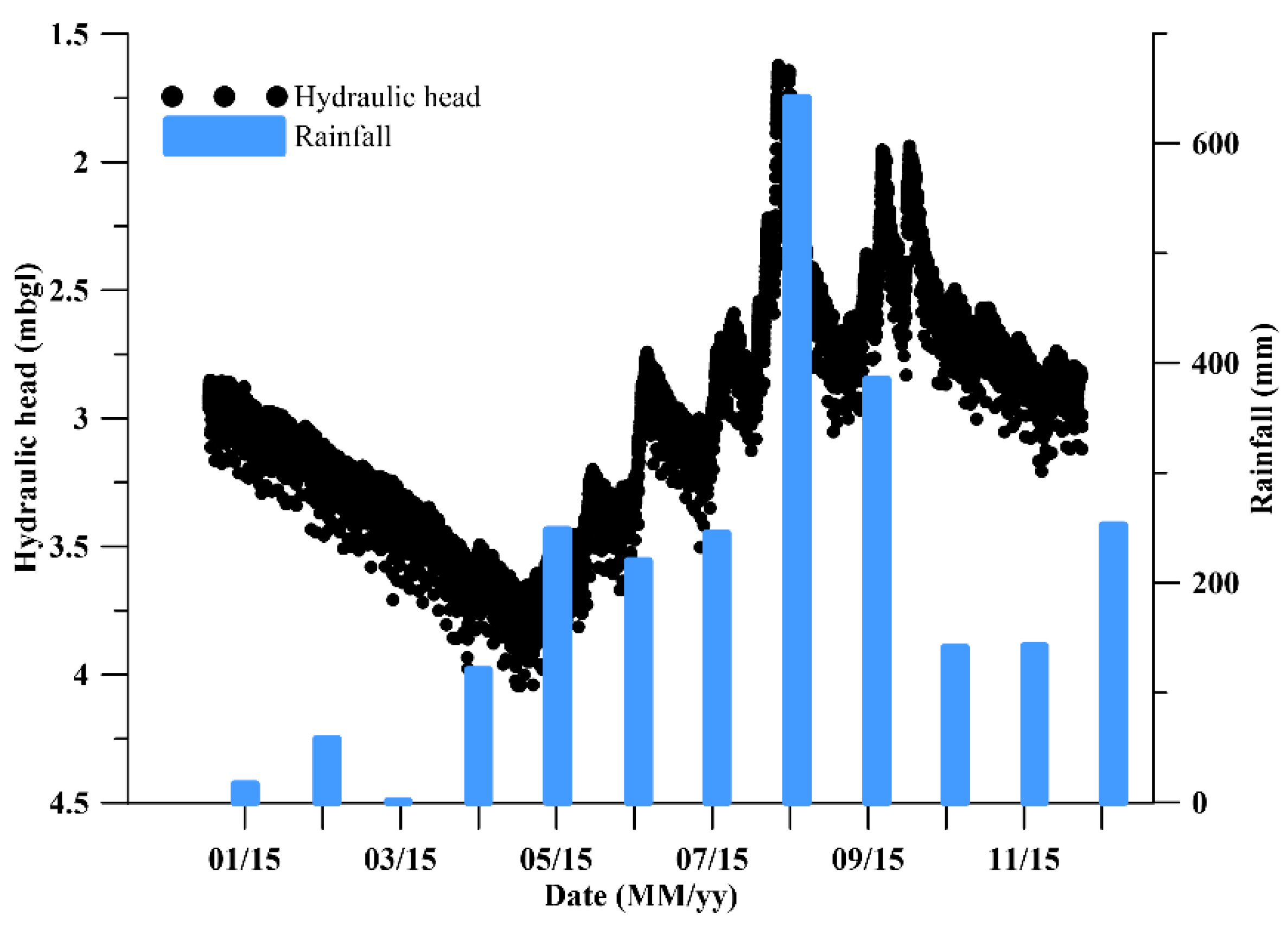Monitoring of water level fluctuation provides information on the dynamics of recharge on a local scale that represents a spatial area of thousands of square meters [2]. In Thepkasattri, a piezometer installed by DGR was used to observe the water table fluctuation pattern. 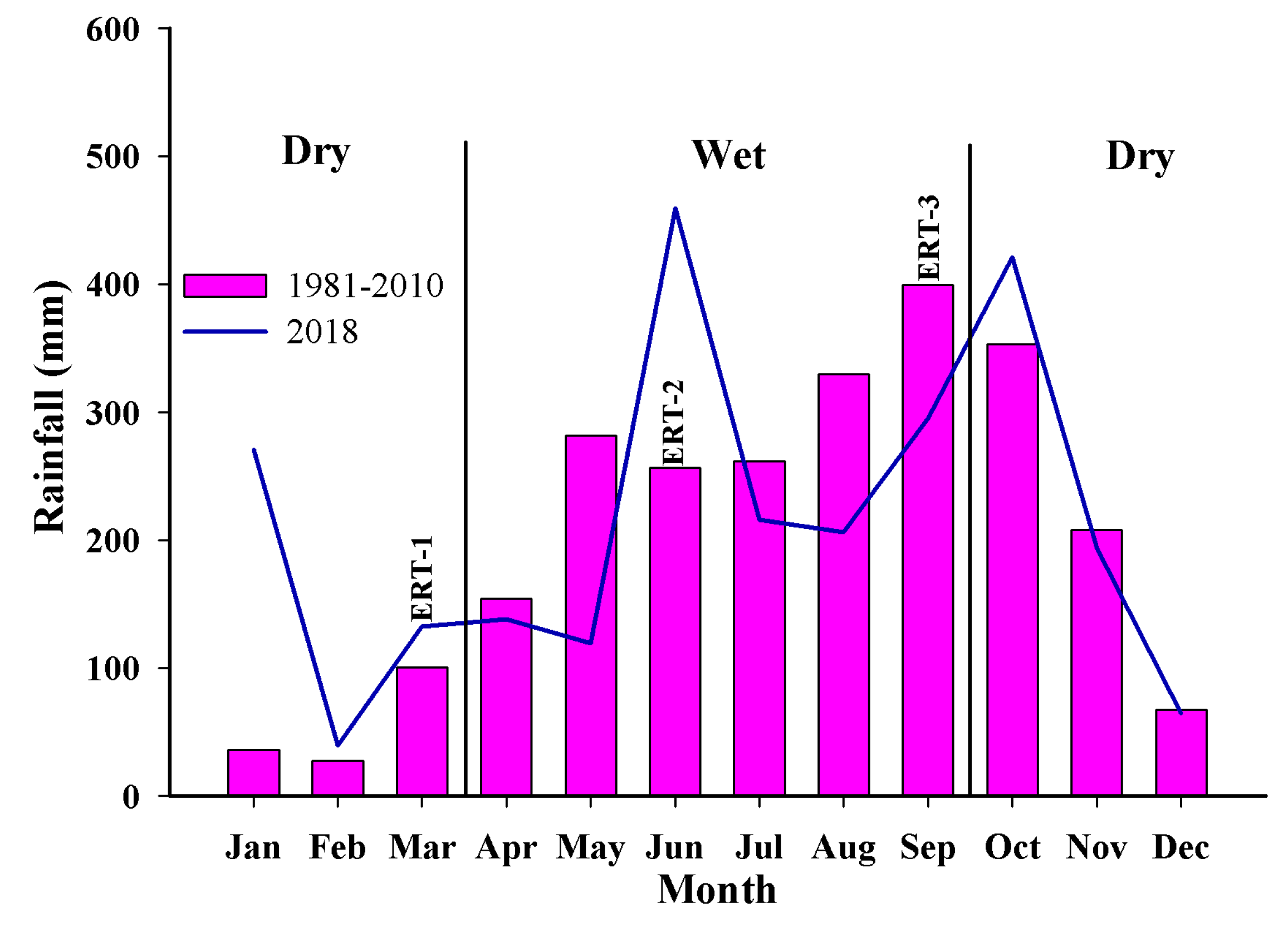The well hydrograph was plotted against average monthly rainfall for 2015 (Figure 5). The data may not be up-to-date, but the climatological information is very similar. In the study area, mean monthly temperature and humidity do not deviate much. The total annual rainfall in 2015 and 2018 was 2472 mm and 2557 mm respectively.

The water table fluctuation dynamics at Wat Phra Thong station follows the rainfall variation of the study area (Figure 5). The hydraulic head reached the deepest level of 4.15 m between March and April (dry season), then started to rise during the wet season and reached the peak (~1.65 m) between July and September. The relationship between water level fluctuation and rainfall suggests the dependency of recharge on the rainfall pattern of the study area. This relationship further implies significant variations in resistivity of the subsurface during the onset of wet season as anticipated.

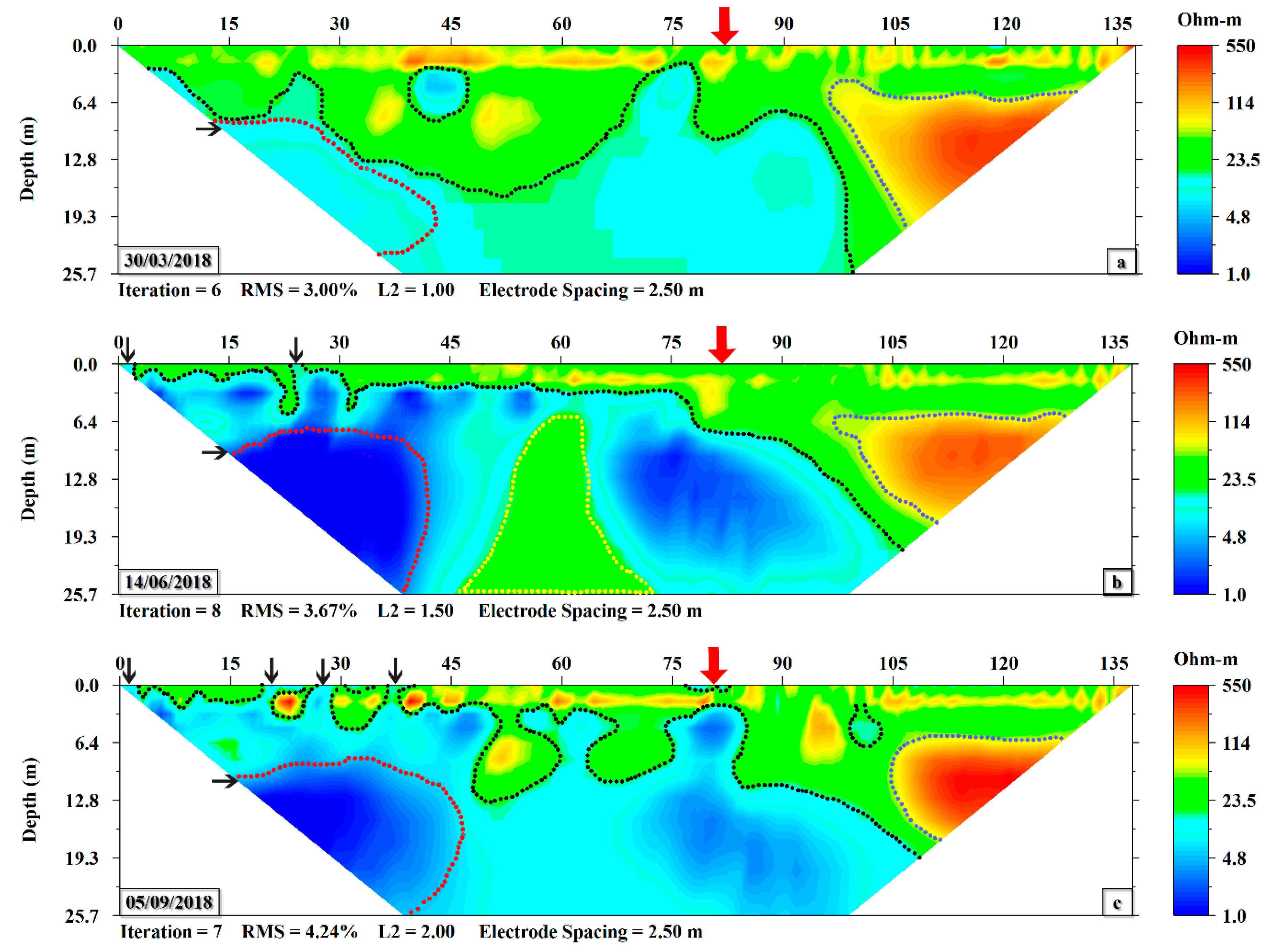
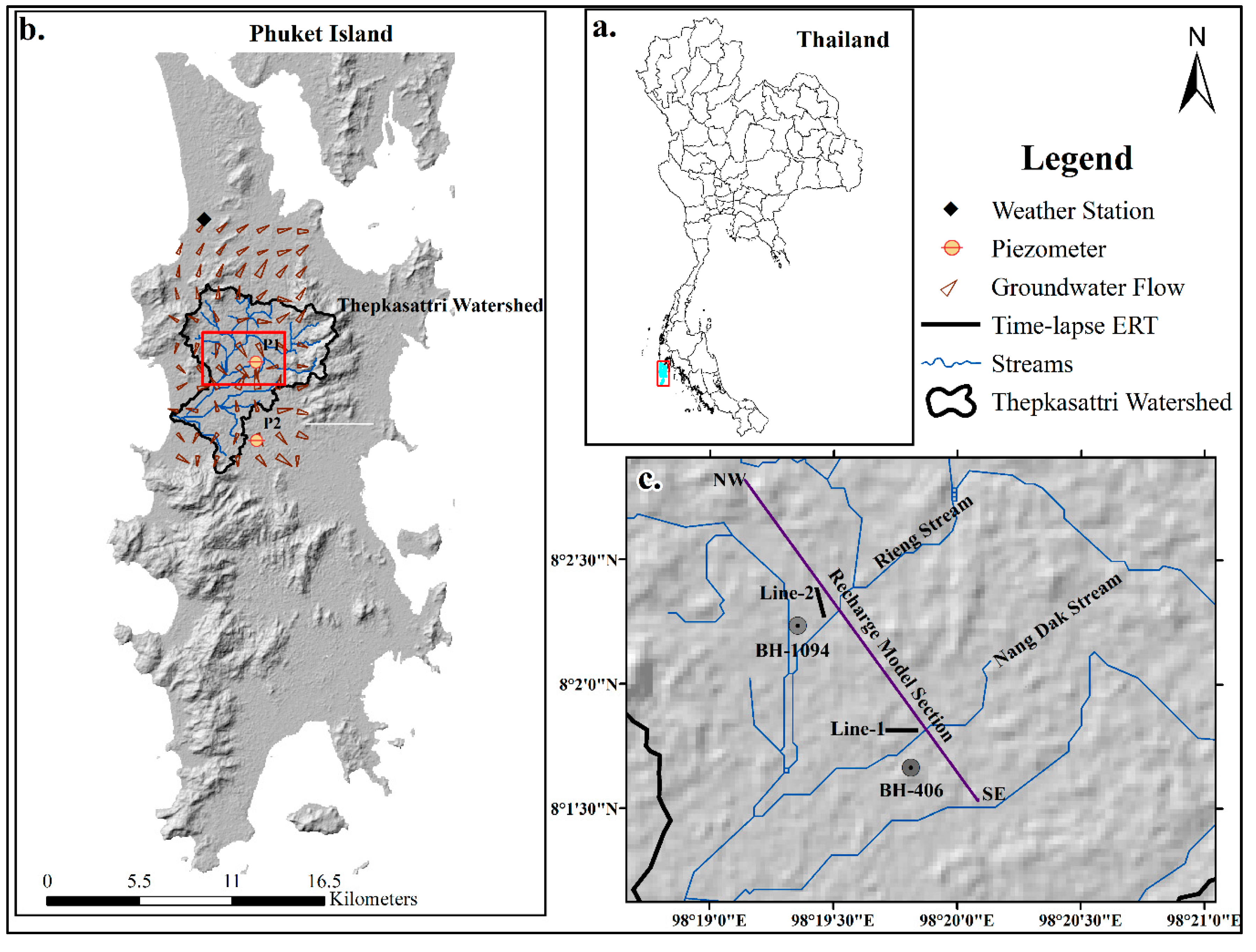
The inversion of line one ERT (alongside Nang Dak stream) is characterized by three horizons as shown in Figure 6. The first horizon represented by blue color has a resistivity range from 4.8 Ωm to 13 Ωm (low resistivity). It is associated with water flux (demarcated by black dotted lines). In the tomography for March (Figure 6a), the low resistivity zone does not extend up to the surface but vertically extends from 3.2 m to the bottom of the profile (demarcated by black dotted lines). The absence of this horizon up to the surface is due to the lack of rain, but the horizon can be distinguished at depth (marked by a horizontal black arrow) extending from the beginning of the profile (0 m) where the Nang Dak stream passes to the distance of 54 m. The presence of this horizon suggests that water infiltration comes from the Nang Dak stream which is located southeast of the survey line (Figure 1c). In (b) and (c) of Figure 6, the low resistivity horizon extends up to the surface (marked by a black arrow) which is due to superficial infiltration in response to rainfall from April to September. The effect of the Nang Dak stream water infiltration is pronounced at this time, with apparent inverted resistivity decrease (demarcated by a red dotted line). The decreasing resistivity value implies that more water flux is coming from the Nang Dak stream to the aquifer.

The low resistivity zone located at a distance between 45 m and 75 m, and a depth from 6.4 m to the 25.7 m (demarcated by yellow dotted lines in Figure 6b) was visible in the March profile, disappeared in June and then re-emerged in September (Figure 6). The inconsistency of the June profile at depth is associated with poorly fit datum points exterminated during ERT inversion (see Supplementary Materials). The bad datum points are due to high contact resistance between the electrode and ground or bad electrodes. The number of iterations used to fit measured and predicted resistivity was eight. Fitting the measured resistivity with predicted resistivity was somewhat difficult (

Table 2. Electrical resistivity inversion statistics: number of iterations and root mean squared (RMS) error.

Date (dd/mm/yyyy)	Array	Iterations		RMS (%)
		Line 1	Line 2	Line 1	Line 2
30/03/2018	Wenner	6	3	3.00	2.50
14/06/2018	Wenner	8	3	3.67	2.51
05/09/2018	Wenner	7	4	3.20	2.61

).

The second major horizon represented by green and yellow colors has resistivity ranging from 20 Ωm to 114 Ωm (medium resistivity). This layer associated with alluvial deposits consists of clayey sand and sandy gravel. The top part of this horizon has an undulating shape due to surficial water infiltration.

The third horizon is the most resistive layer (demarcated by a blue dotted line) located at 97 m to the end of the profile distance, and vertically from 6.2 m to 19.3 m (Figure 6). The resistivity of this layer ranges from 200 Ωm to 550 Ωm. The resistive body located at distances from 105 m onwards might be a 3D artifact associated with minor elevation change [3], or it might be due to dry or impermeable rock.

3.2. Thepkasattri Line Two Alongside the Rieng Stream

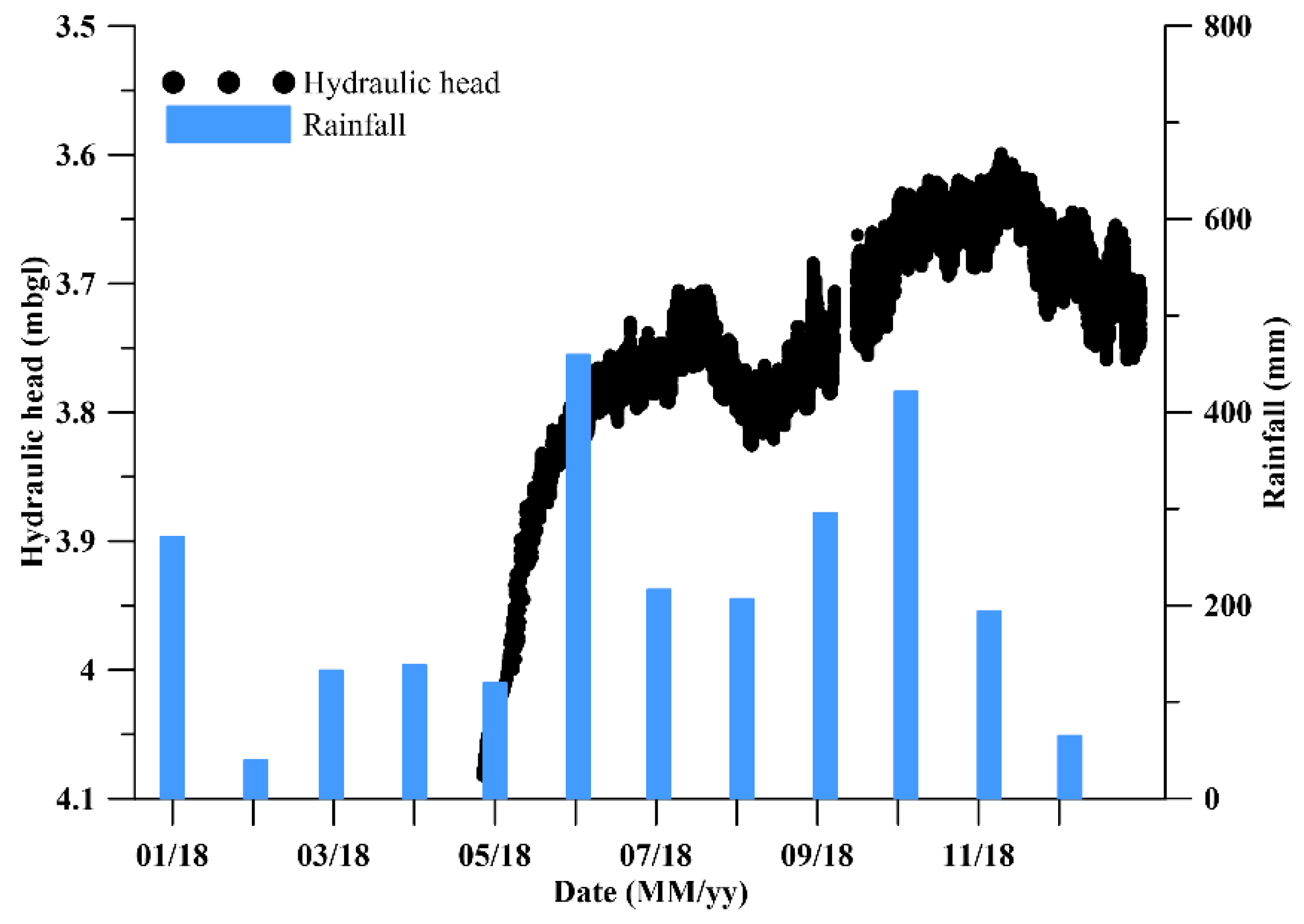
A piezometer coupled with rain gauge installed in May 2018 at CDPM station was used to observe water table fluctuation pattern during the ERT survey time. The piezometer recorded water level and rainfall on an hourly basis throughout the day. The well hydrograph along with the variation of rainfall in the study area is shown in Figure 7. It is apparent from the figure that there is an association between water level rise and the amount of rainfall. Water level started to rise in May, corresponding to the onset of the rainy season reaching peak value of 3.6 m (bgl) at the end of the season. The peak water level corresponds to the highest rainfall recorded in September and October. This association further indicates that recharge is episodic and it depends on the amount of rainfall and the hydraulic property of the vadose zone.

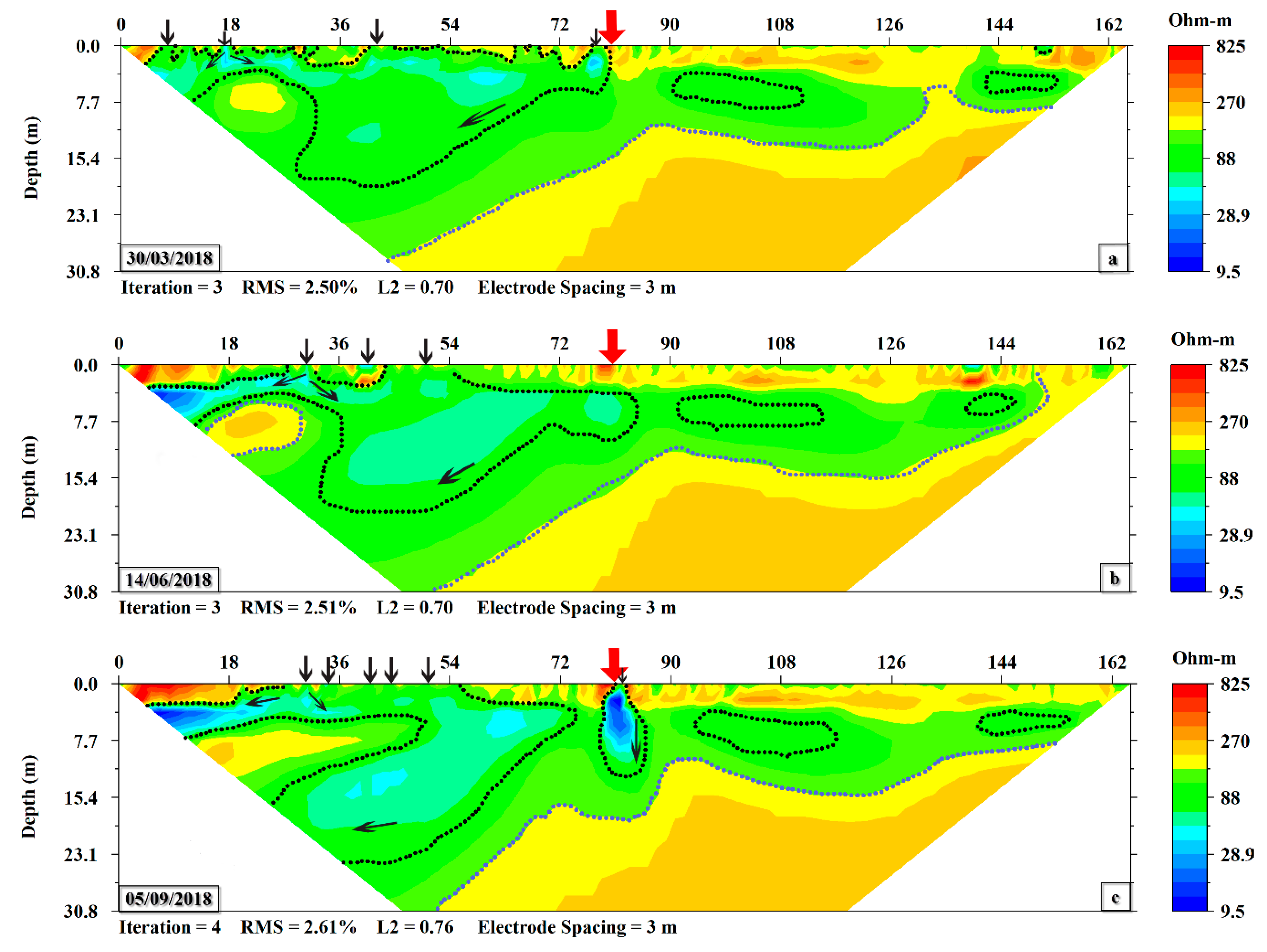
The inversion result of line two alongside the Rieng stream shows that the tomography is dominated by two horizons as shown in Figure 8. The low resistivity zone is represented by green and irregularly distributed blue colors (demarcated by black dotted lines). The resistivity in this zone ranges from 9.5 Ωm to 100 Ωm. The zone extends to a depth of 23.1 m at a 36 m distance, and from that distance the layer pinches out. At distances of 139 m to 157 m, the layer was found only to a depth of 7.7 m in all profiles. This zone is associated with the weathered part of granite bedrock functioning as an aquifer. However, the zone slightly increased vertically in the June to September profiles, and this change is associated with moisture movement in the vadose zone.

The most conductive zone (dark to light blue color) with resistivities from 9.5 Ωm to 40 Ωm shows variations in shape across the three dates (March, June, and September). The variation is prominent in the June and September profiles as shown in the three tomographies (Figure 8, demarcated by black dotted lines). The overall variation of the zone indicates water flux movement. At the distance of 81 m (marked by red arrow), the zone extends from 3 m depth in March to around 12 m depth in September. The extension of the low resistivity indicates the vertical movement of water in the vadose zone. Similarly, the low resistivity horizon shows variation between 18 m and 68 m distance (marked by inclined black arrows), indicating water infiltration both vertically and horizontally. In this profile, there is a crescent shape conductive zone associated with preferential flow from the vadose zone at 18 m marked by vertical black arrows in (b) and (c) of Figure 8. The resistivity changes in the profiles indicate groundwater flow into the Rieng stream located on the left parts of the profiles. In this area, the average groundwater level is 4.0 m (bgl), varying by about 1 m below or above the Rieng stream bed, depending on the season. This implies that groundwater is discharging as a base flow through the Rieng stream.

The second dominant zone represented by yellow/red color and demarcated by a blue dotted line has resistivity range from 200 Ωm to 825 Ωm. This zone dominates the left side of the profile. The horizon regularly extends from 40 m to 165 m. This zone is interpreted to represent granite bedrock and can be easily identified in the well log data and resistivity log (Figure 2 and Figure 9b).

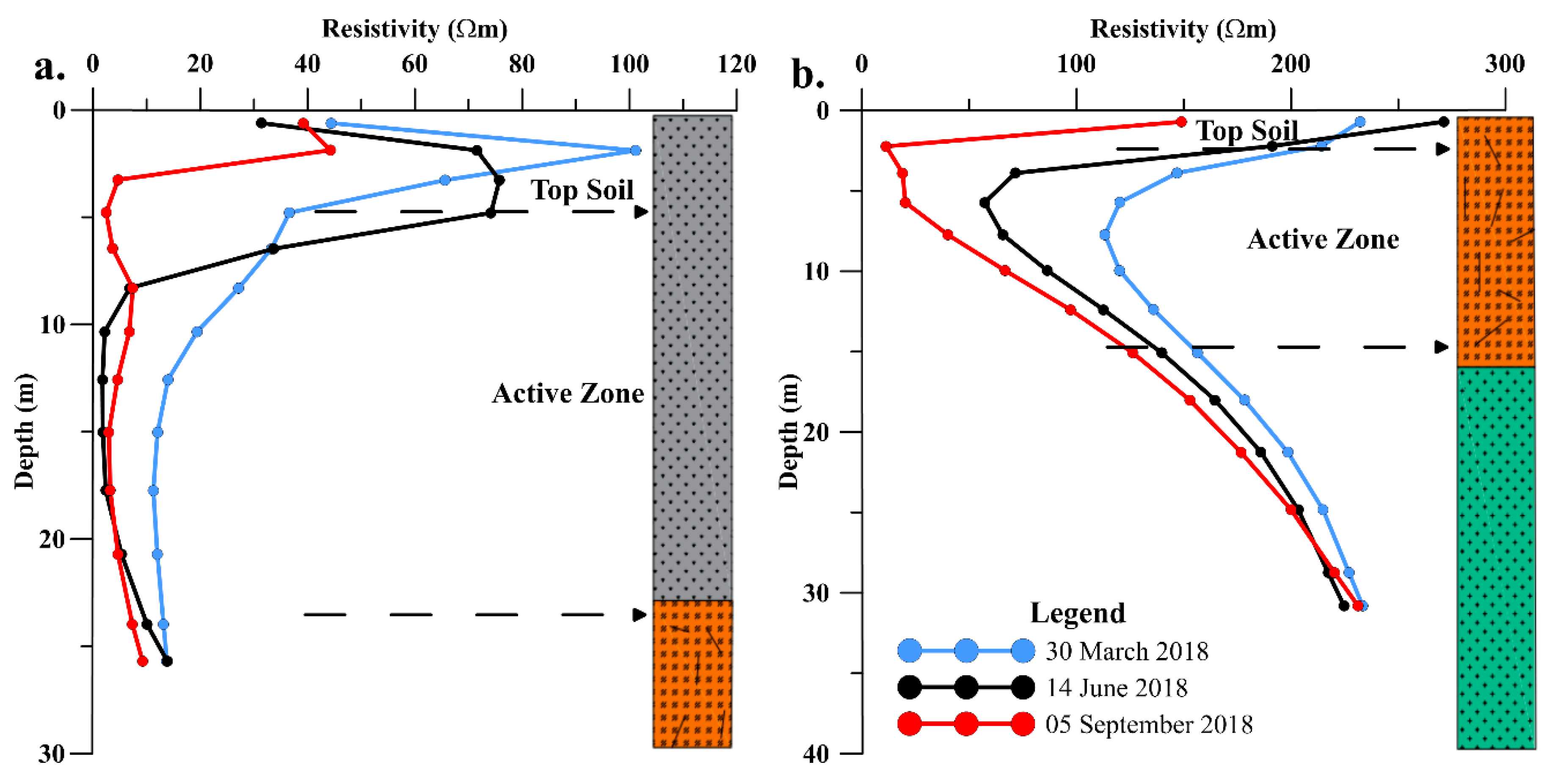
The use of resistivity log is helpful in outlining the geologic layers and active zones characterized by major resistivity change in monitoring datasets [13]. As Alamry et al. [13] reported the top soil is characterized by uneven resistivity distribution indicating vegetation soil interaction, while the active zone represents uniform resistivity change throughout the survey dates, indicating water movement. Therefore, a resistivity log at a distance of 81 m (marked by the red arrow in Figure 6 and Figure 8) was extracted to confirm the geological layers and demarcate the active zone represented by significant variations in resistivity. The resistivity log of line one is shown in Figure 9a; the top soil is characterized by variable resistivity associated with the variability of water saturation due to evapotranspiration. The thickness of this layer is around 5 m. The second layer is the active zone characterized by major resistivity change among the three dates. This layer has a thickness of 17 m, and beyond that depth, the resistivity log does not show a significant difference among the three dates.

The resistivity log for line two at a distance of 81 m is shown in Figure 9b. The top soil represented by variable resistivity value has a thickness of around 3 m. The active zone is much thinner in line two than line one, which is due to the high permeability, and the porosity zone is thicker in line one. In both resistivity logs, the layer below the active zone is characterized by almost no resistivity change, indicating the bedrock.

3.3. Line One Time-Lapse ERT

Time-lapse inversion was done using EarthImager 2D 2.4.4 following the standard procedures in the manual [14]. The Smooth model inversion was used for all time-lapse ERT inversions. The time-lapse ERT data were inverted by setting the dry season profile as the base model for the following June and September profiles, as recommended by Miller et al. [6]. Finally, the inversion produces a percentage difference in resistivity between the base and monitoring datasets.

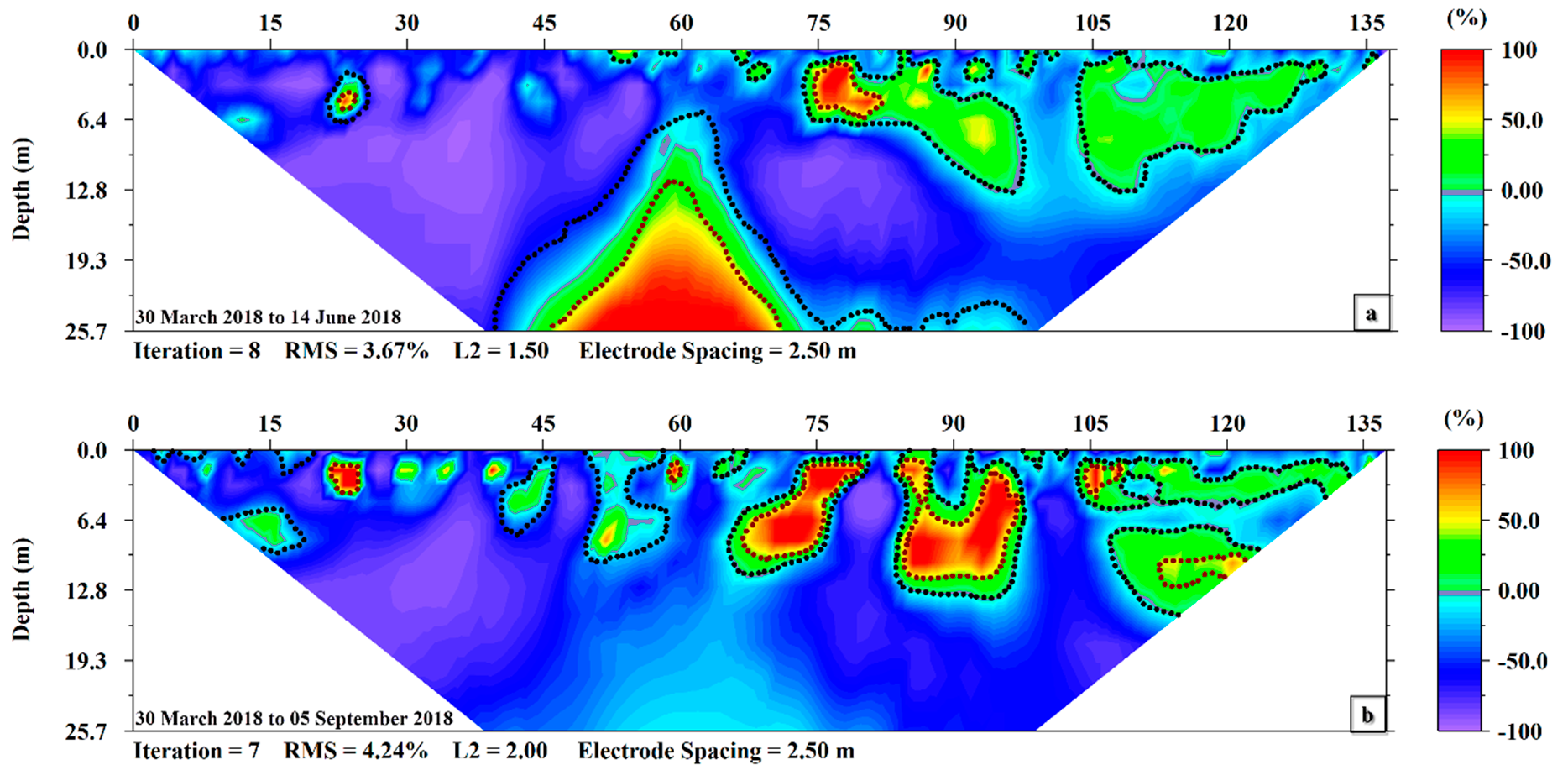
Time-lapse ERT inversion of line one from March to June and March to September are shown in Figure 10. On the right side of both profiles, up to a distance of 135 m, there are strong resistivity decreases from −50% to −100% (demarcated by black dotted lines). The strong resistivity change extends from the surface to the bottom of the profile. The change implies water infiltration through the vadose zone during the rainy season; the percentage variation in resistivity indirectly indicates the volume of water occupying the pore spaces [6]. The consistency of the time-lapse ERT in both dates indicates infiltration from the surface, and the Nang Dak stream is the preferential recharge zone for the aquifer. The preferential recharge zones are regularly connected with the bottom aquifer throughout the profile, forming funneled flow. Superficially continuous resistivity decrease throughout the profile in the sedimentary vadose zone is also reported by Mojica et al. and Zhang et al. [7,15]. The nature of the preferential flow suggests the hydraulic heterogeneity of the alluvial deposit. However, in (Figure 10b) the preferential flow occurs as patches to a depth of 9.6 m. This irregularity is associated with artifacts caused by the relocation of electrodes and bad datum points.

The resistive layer represented by the yellow to red color and demarcated by the brown dotted line shows a strong resistivity increase by 50% to 100%. In Figure 10a, a resistive body is located at distances from 48 m to 72 m and vertically from 12.8 m to the bottom of the profile (demarcated by brown dotted lines). This layer later disappeared in the March–September time-lapse inversion (Figure 10b). This implies that the resistive layer is caused by bad datasets in the June profile as described in Section 3.1. In addition, in Figure 10a, an increase in resistivity is shown at a 75 m distance and between 1 m to 6.4 m deep, and, in Figure 10b, irregularly distributed from 22 m to 97 m distances and 9.6 m deep. The increase in resistivity is associated with a time-lapse inversion artifact caused by moisture contrast between the dry and wet season. The inversion artifacts are false results caused by the inversion model’s incapability to fit the contrasting resistivity values during time-lapse inversion [4]. In addition, there is a resistivity decrease at depth in both time-lapse ERT that might be due to enrichment in the ionic concentration of groundwater [16]. On the other hand, it might be due to the effect of the overlying material electrical property or poor model resolution at depth [15,16,17,18].

3.4. Line Two Time-Lapse ERT

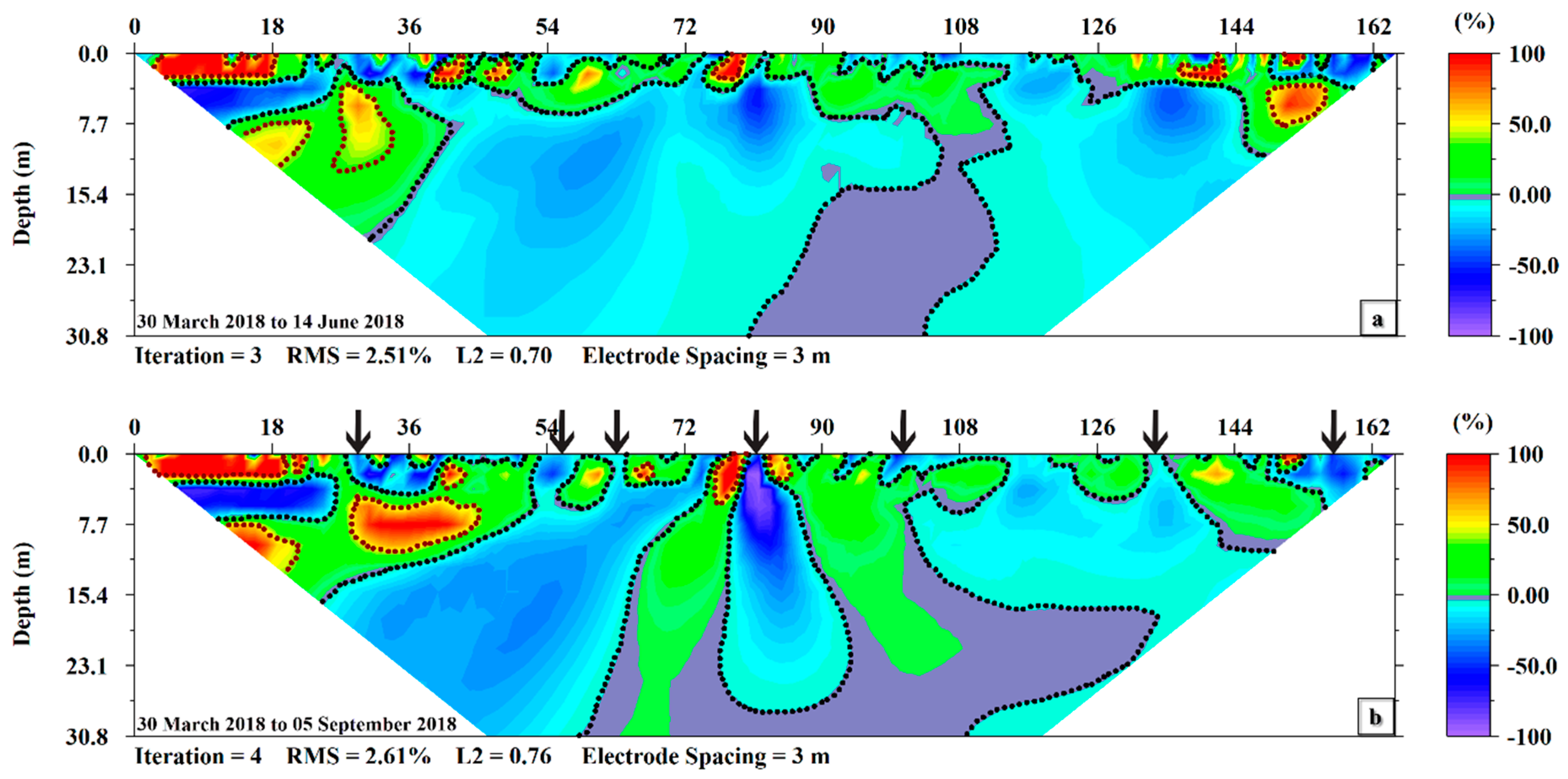
Time-lapse ERT inversions of line two data for March to June and March to September comparisons are shown in Figure 11. These profiles are dominated by less than 75% resistivity decreases demarcated by black dotted lines. These strong resistivity changes are associated with the first rainfall in the rainy season. In Figure 11a, the resistivity decrease is attributed to preferential recharge zones located between 27 m and 122 m distance. Similarly, the consistency of those preferential recharge zones is observed in the March to September time-lapse inversion as well. The presence of consistent preferential recharge zones supports the concept that recharge in weathered/fractured granite is mainly controlled by slowly moving wetting fronts and well-connected fractures [19]. The top part of the tomography is characterized by unstable flow concentrated into conductive fingers in March to June time-lapse ERT (Figure 11a). Then some conductive fingers become preferential recharge zones (marked by black arrow at X = 27 m, 54 m, 63 m, 81 m, 104 m, 135 m and 157 m) in the March to September time-lapse ERT (Figure 11b). At an 81 m distance, the wetting front is penetrating vertically downward to a depth of around 29 m, indicating a well-connected fracture zone. Similarly, in all distances marked by a black arrow, the infiltrated water follows uniform pathways (preferential recharge zones) to reach the other parts of the profile. This implies structurally controlled infiltration pathways typical of fractured hard rocks [18,19,20]. Robert et al. [21] also found structurally controlled preferential recharge zones in an investigation done in fractured/karstified limestones (southern Belgium). The study was done by injecting salt tracer to map flow paths using time-lapse ERT. The complicated preferential flow in the vadose zone is associated with textural heterogeneity and hydraulic properties of the weathered granite layer [22].

The resistivity increased from 5% to 50% in a layer that mainly occurs at the top part of the profile and the left side of the profile from a distance of 9 m to 40 m and at depths from 3 m to 21 m. This layer is associated with a low permeability body that is part of the granite bedrock. Then, later on, the time-lapse ERT of March to September shows that the layer seems to decrease vertically by 4 m due to deep percolation of water. Furthermore, there is a resistive body characterized by 70% to 100% resistivity increase found between the top surface and 11 m depth (demarcated by a brown dotted lines). This resistive layer is an inversion artifact associated with changes in moisture content or with the relocation of electrodes during those dates [4,6,7].

The resistivity variations between dry and wet seasons are much higher for line one than for line two. There was around 100% resistivity decrease in line one, while in line two there was a 75% decrease. Based on petrophysical transformation, the change in resistivity (electrical conductivity) can be related to the degree of water saturation. As the Miller et al. [6] study in Dry Creek watershed has shown, an increase in electrical conductivity corresponds to an increase in water saturation. Therefore, it can be inferred that the degrees of saturation in both locations are different. Geologically, the vadose zone in line one is an alluvial deposit and is weathered/fractured granite in line two (Figure 2). This indicates that in weathered and fractured granite, the recharge is controlled by slowly draining wetting fronts (flow paths) as revealed in the three tomograms and time-lapse ERT (see Figure 8 and Figure 11). Structurally controlled wetting fronts are also identified in hard rocks by previous researchers [3,19]. As Arora et al. [3] reported, in vadose zones consisting of fractured/weathered granite, water movement is both horizontal and vertical. The result was further confirmed by self-potential survey and in situ soil moisture profiling.

Furthermore, the interannual change in the well hydrograph correlates considerably with interannual rainfall pattern of the study area. In addition, time-lapse ERT shows strong seasonal resistivity variation in the vadose zone, indicating water infiltration during the rainy season. The relationship suggests that groundwater recharge is dependent on the annual rainfall pattern of the study area [23,24]. As Wu et al. [23] investigated, the relationship between annual recharge and rainfall is significant for shallow groundwater depths, which is the case in the Thepkasattri watershed.

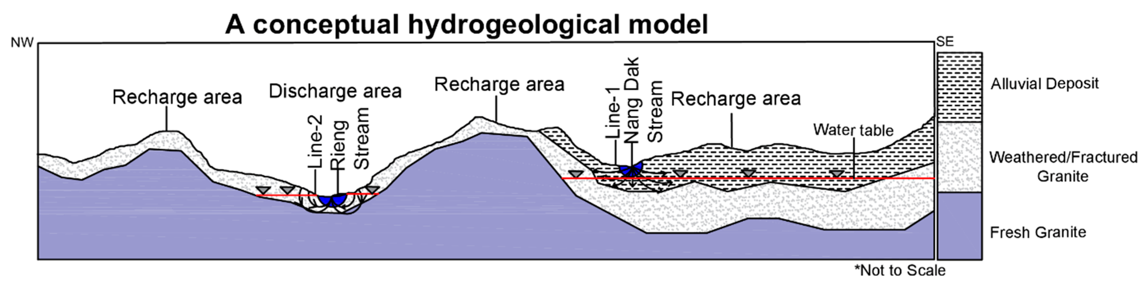
3.5. A Conceptual Hydrogeological Model

Based on the hydrogeological information of the study area and the time-lapse ERT result, a conceptual hydrogeological model was drawn along an NW–SE cross-section to visualize the recharge mechanism in the study area (Figure 1c). The hydrogeological information was taken from groundwater data provided by DGR, ERT results, and field observation. The thickness of the geological layers is not to scale; it was inferred based on well log and field observation. Then the available information was used to make the conceptual hydrogeological model using AutoCAD 2017 software (Figure 12).

A conceptual hydrogeological model of the study area shows the topographic highs including the stream passing nearby line one are groundwater recharge areas. Generally, the topographic highs in the study have a gentle slope favorable for diffuse recharge [2]. The topographic lows near line two are groundwater discharge zones as base flow.

Seasonal groundwater recharge in the Thepkasatri watershed varies based on the geology of the vadose zone and rainfall pattern. The time-lapse ERT in both locations further suggests that water movement is mainly controlled by hydraulic heterogeneity and fracture pattern of the vadose zone.

4. Conclusions

Time-lapse ERT coupled with well hydrograph was applied to investigate the seasonal groundwater recharge variations in the Thepkasattri watershed. Time-lapse ERT is a non-destructive method and provides information on spatial and temporal variations of water infiltration in the vadose zone. Water table fluctuation observation and well log data were used to determine recharge variation throughout the seasons and provide subsurface geological information, respectively. The integration of hydrogeological and geophysical data in the study area was useful for ERT interpretation. The time-lapse ERT method also has limitations that require care during data interpretations. These are artifact generation during inversion and relocation of electrodes [4,6]. The well hydrograph of the area indicates recharge is seasonal and dependent on the rainfall pattern. Similarly, the seasonal variations in groundwater recharge (moisture content) in the time-lapse ERT are expressed as differences in resistivity between the base model and the monitoring datasets. In line one and line two of the tomography, strong seasonal resistivity variations were observed in the vadose zone. The maximum resistivity decrease in line one reaches around 100%, while in line two it was 75% or less. The decrease in resistivity is strongly related to infiltration from rainfall during the rainy season. Based on the water table fluctuation datasets and time-lapse ERT, the aquifer replenishment in the study area is mainly caused by superficial water infiltration that depends on the rainfall pattern of the study area. This study demonstrated applicability and utilization of time-lapse ERT method to visualize moisture variation in soil and to identify preferential recharge zones. The well-resolved time-lapse images in two contrasting unsaturated zones further indicate the potential of the method to provide noninvasive spatiotemporal moisture variation in the vadose zone.

References

1. Williams, M. What Percent of Earth is Water? Available online: https://www.universetoday.com/65588/what-percent-of-earth-is-water/ (accessed on 3 March 2018).
2. Healy, R. Estimating Groundwater Recharge, 1st ed.; Cambridge University Press: Cambridge, UK, 2012; pp. 1–13. [Google Scholar]
3. Arora, T.; Ahmed, S. Characterization of recharge through complex vadose zone of a granitic aquifer by time-lapse electrical resistivity tomography. J. Appl. Geophys. 2011, 73, 35–44. [Google Scholar] [CrossRef]
4. Carey, A.M.; Paige, G.B.; Carr, B.J.; Dogan, M. Forward modeling to investigate inversion artifacts resulting from time-lapse electrical resistivity tomography during rainfall simulations. J. Appl. Geophys. 2017, 145, 39–49. [Google Scholar] [CrossRef]
5. Descloitres, M.; Ruiz, L.; Sekhar, M.; Legchenko, A.; Braun, J.J.; Kumar, M.S.; Subramanian, S. Characterization of seasonal local recharge using electrical resistivity tomography and magnetic resonance sounding. Hydrol. Process. 2007, 22, 384–394. [Google Scholar] [CrossRef]
6. Miller, C.R.; Routh, P.S.; Brosten, T.R.; McNamara, J.P. Application of time-lapse ERT imaging to watershed characterization. Geophysics 2008, 73, G7–G17. [Google Scholar] [CrossRef]
7. Mojica, A.; Diaz, I.; Ho, C.A.; Ogden, F.; Pinzon, R.; Fabrega, J.; Vega, D.; Hendrickx, J. Study of seasonal rainfall infiltration via time-lapse surface electrical resistivity tomography: Case study of Gamboa area, Panama Canal Watershed. Air Soil Water Res. 2013, 6, 131–139. [Google Scholar] [CrossRef]
8. Hummel, C.L.; Phawandon, P. Geology and Mineral Deposits of the Phuket Mining District, South Thailand; Department of Mineral Resources: Bangkok, Thailand, 1967.
9. Charoenpong, S.; Suwanprasit, P.; Thongchumnum, P. Impacts of interpolation techniques on groundwater potential modeling using GIS in Phuket Province, Thailand. In Proceedings of the 33rd ACRS, Pattaya, Thailand, 26–30 November 2012; pp. 732–738. [Google Scholar]
10. Kong, S.O. Hydrogeological Characterization of Phuket Aquifer System with Reference to Groundwater Development of Phuket, Thailand. Master’s Thesis, Prince Songkla University, Phuket, Thailand, 2017. [Google Scholar]
11. Loke, M.H.; Acworth, I.; Dahlin, T. A comparison of smooth and blocky inversion methods in 2D electrical imaging method. Explor. Geophys. 2003, 34, 182–187. [Google Scholar] [CrossRef]
12. Healy, R.; Cook, P. Using groundwater levels to estimate recharge. Hydrogeol. J. 2002, 10, 91–109. [Google Scholar] [CrossRef]
13. Alamry, A.S.; van der Meijde, M.; Noomen, M.; Addink, E.A.; van Benthem, R.; de Jong, S.M. Spatial and temporal monitoring of soil moisture using surface electrical resistivity tomography in Mediterranean soils. Catena 2017, 157, 388–396. [Google Scholar] [CrossRef]
14. Advanced Geoscience Inc. Instruction Manual for EarthImager 2D Version 2.4.0; Advanced Geoscience Inc.: Austin, TX, USA, 2014; Vol. 2.4.0. [Google Scholar]
15. Zhang, G.; Zhang, G.; Chen, C.; Chang, P.; Wang, T.; Yen, H.; Dong, J.; Ni, C.; Chen, S.; Chen, C.; et al. Imaging rainfall infiltration process with the time-lapse electrical resistivity imaging method. Pure Appl. Geophys. 2016, 173, 2227–2239. [Google Scholar] [CrossRef]
16. Clément, R.; Descloitres, M.; Günther, T.; Ribolzi, O.; Legchenko, A. Influence of shallow infiltration on time-lapse ERT: Experience of advanced interpretation. Comptes Rendus - Geosci. 2009, 341, 886–898. [Google Scholar] [CrossRef]
17. Loke, M.H. Electrical Imaging Surveys for Environmental and Engineering Studies: A Practical Guide to 2-D and 3-D Surveys. Available online: https://www.semanticscholar.org/paper/Electrical-Imaging-Surveys-for-Environmental-and-Loke/efa943ffb44f5a217e2d22255f7e334778932248 (accessed on 2 May 2019).
18. Pellicer, X.M.; Zarroca, M.; Gibson, P. Time-lapse resistivity analysis of Quaternary sediments in the Midlands of Ireland. J. Appl. Geophys. 2012, 82, 46–58. [Google Scholar] [CrossRef]
19. Gleeson, T.; Novakowski, K.; Kurt Kyser, T. Extremely rapid and localized recharge to a fractured rock aquifer. J. Hydrol. 2009, 376, 496–509. [Google Scholar] [CrossRef]
20. Ulusoy, İ.; Dahlin, T.; Bergman, B. Time-lapse electrical resistivity tomography of a water infiltration test on Johannishus Esker, Sweden. Hydrogeol. J. 2015, 23, 551–566. [Google Scholar] [CrossRef]
21. Robert, T.; Caterina, D.; Deceuster, J.; Kaufmann, O.; Nguyen, F. A salt tracer test monitored with surface ERT to detect preferential flow and transport paths in fractured/karstified limestones. Geophysics 2012, 77, B55–B67. [Google Scholar] [CrossRef]
22. Nimmo, J.R. Vadose water. Encycl. Inl. Waters. 2009, 1, 766–777. [Google Scholar] [CrossRef]
23. Wu, J.; Zhang, R.; Yang, J. Analysis of rainfall-recharge relationships. J. Hydrol. 1996, 177, 143–160. [Google Scholar] [CrossRef]
24. Kotchoni, D.O.V.; Vouillamoz, J.M.; Lawson, F.M.A.; Adjomayi, P.; Boukari, M.; Taylor, R.G. Relationships between rainfall and groundwater recharge in seasonally humid Benin: A comparative analysis of long-term hydrographs in sedimentary and crystalline aquifers. Hydrogeol. J. 2018, 27, 447–457. [Google Scholar] [CrossRef]
Figure 1. Maps of the study area and groundwater flow directions. (a) Thailand map, the highlighted red box shows Phuket Island; (b) Phuket Island, the red box indicates the location of the study area, weather station and piezometer (P1: Wat Phra Thong, P2: College of Disaster Prevention and Mitigation (CDPM); (c) Electrical resistivity tomography (ERT) survey lines (Line-1: alongside Nang Dak stream and Line-2: alongside Rieng stream), boreholes (BH) and recharge model sections.
Hydrology 06 00036 g001
Figure 2. Geology of the subsurface layers from well log data. a.s.l. = above sea level.
Hydrology 06 00036 g002
Figure 3. A schematic diagram of the Wenner array electrode configuration. ‘A’ and ‘B’ = current electrodes (I = current), ‘M’ and ‘N’ = potential electrodes (V = potential difference) and ‘a’ = spacing between electrodes.
Hydrology 06 00036 g003
Figure 4. Mean total monthly rainfall. The bar chart shows mean total monthly rainfall from 1981 to 2010, line plot shows total monthly rainfall for 2018 from a weather station in the study area. The ERT survey months are indicated on the top of the relevant bars.
Hydrology 06 00036 g004
Figure 5. A chart showing water table fluctuation versus the total monthly rainfall in 2015 from a station at Wat Phra Thong. mbgl = meters below ground level.
Hydrology 06 00036 g005
Figure 6. Electrical resistivity tomography of line one. The red arrow indicates the location of resistivity log at 81 m distance: (a) 30 March 2018; (b) 14 June 2018; (c) 05 September 2018. RMS = root mean squared error; L2-norm = the sum of the squared weighted data errors.
Hydrology 06 00036 g006
Figure 7. A chart showing water table fluctuation versus average monthly rainfall in 2018 from a station at CDPM.
Hydrology 06 00036 g007
Figure 8. Electrical resistivity tomography of line two. The red arrow indicates location of resistivity log at 81m distance: (a) 30 March 2018; (b) 14 June 2018; (c) 05 September 2018.
Hydrology 06 00036 g008
Figure 9. Showing the resistivity log extracted at an 81 m distance (Figure 6 and Figure 8). Top soil is characterized by root and soil interaction and the active zone is characterized by uniform resistivity change. (a) Resistivity log of line one; (b) Resistivity log of line two.
Hydrology 06 00036 g009
Figure 10. Time-lapse inversion of line one with root mean squared (RMS) error: (a) 30 March 2018 to 14 June 2018; (b) 30 March 2018 to 05 September 2018.
Hydrology 06 00036 g010
Figure 11. Time-lapse inversion of line two with root mean squared (RMS) error: (a) 30 March 2018 to 14 June 2018; (b) 30 March 2018 to 05 September 2018.
Hydrology 06 00036 g011
Figure 12. A simplified conceptual hydrogeological model of the study area.
Hydrology 06 00036 g012