Transport and Fate of Nitrate in the Streambed of a Low-Gradient Stream

Abstract

The transport and fate of nitrate (NO₃⁻) to in the top 15 cm of a streambed has been well-documented, but an understanding of greater depths is limited. This work examines the transport and fate of nitrate (NO₃⁻) at depths of 30 cm, 60 cm, 90 cm, and 150 cm below the stream-streambed interface. Concentrations of nitrate as nitrogen (NO₃-N) and chloride (Cl⁻) were measured in the waters from the streambed, the stream water, and the groundwater. Mixing models predicted values of ΔNO₃-N, the difference between measured NO₃-N and theoretical NO₃-N. At a 30-cm depth, the mean ΔNO₃-N value was −0.25 mg/L, indicating a deficit of NO₃-N and the removal of NO₃-N from the system. At deeper levels, the values of ΔNO₃-N began to approach zero, reaching a mean value of −0.07 mg/L at 150 cm. The reduction of NO₃-N does not appear to be controlled by vegetation, as it was not correlated to either temperature or visible light. Larger negative ΔNO₃-N values (more removal) occur when stream NO₃-N concentrations are higher and organic matter is present.

1. Introduction

Fertile soils within the upper Mississippi River Basin experience intensive agricultural practices that utilize nitrogen (N) fertilizers to enhance yield. Under optimal growing conditions, crop yield accounts for 50% of the added N; the excess nitrogen remains within or is exported from the system [1]. Since the 1960s, the application of N fertilizers to agricultural fields has increased significantly; subsequently, nitrate as nitrogen (NO₃-N) concentrations in rivers and reservoirs has concurrently increased throughout agricultural regions [2]. Once in the waterways, NO₃-N may be removed by microbial processes in the streambed sediment and by plant uptake [3,4,5]. However, approximately 25% of the NO₃-N in the stream system will remain mobile, eventually discharging into the Gulf of Mexico [6,7]. Since 1950, the NO₃-N load discharged into the Gulf of Mexico has tripled [8,9], with the Illinois River identified as the second leading contributor of NO₃⁻ to the Mississippi River [10], accounting for 19% of the NO₃-N load delivered to the Gulf of Mexico by the Mississippi River [11,12,13]. The increase in N entering the Gulf of Mexico has been correlated to an increase in the frequency and the magnitude of the zone of hypoxia in the Gulf of Mexico and to changes in biodiversity within surface waters [9,14,15,16]. Effects of excess nitrogen are not limited to the United States and are of global concern [17,18,19]. The transport and fate of nitrogen in agricultural watersheds have been well-reported (e.g., [20,21,22,23,24,25,26]). Specifically, the function of the upper portion of the streambed in the nitrogen cycle has received significant attention [27,28,29,30].

The zone within the streambed substrate, where surface water and groundwater mix, exhibits a natural capacity for nitrogen removal [22,28,31,32,33]. Reported NO₃-N removal processes include denitrification and aquatic uptake by in-stream plants and benthic sediments [32,34,35,36,37,38]. Spatial variability in the distribution and composition of microbial communities, the concentrations of dissolved oxygen (DO), the concentration of organic matter (OM), and the concentration and species of nitrogen within the streambed control the rate of N removal [35,39,40,41,42,43]. Longer residence time of the waters in the streambed correlate to enhanced reduction of NO₃-N concentrations [44].

Seasonal variation of NO₃-N concentrations in midwestern streams has been observed [45,46]; the variations are attributed to precipitation, fertilizer application, rate of stream water discharge, and the concentration of dissolved organic carbon in pore water within the streambed [3,4,6]. Concentrations of NO₃-N tend to be higher during early spring following the application of fertilizers and when more frequent and higher magnitude precipitation events increase runoff. Nitrate concentrations are typically lowest during summer, when there is a limited source of NO₃-N and there is increased uptake from growing plants [38,45]. The rate of denitrification, which is lowest during the winter months (November to March) and highest in early spring and summer (April to July), influences the seasonal variation of NO₃-N concentrations in streams [4,47]. Moreover, the decrease in winter denitrification rates is attributed to a decrease in temperature and in microbial activity. Elevated denitrification rates during spring and summer are correlated to increased NO₃-N entering the system and to increased amounts of decaying foliage entering the stream, providing OM for the denitrifying microbes.

Nitrate removal in stream ecosystems is thought to occur disproportionately in zones with long residence times that facilitate the contact of reactive solutes with high biotic capacity for biogeochemical processing [42,48]. Despite studies indicating that significant microbial processes occur up to several meters below the streambed, the majority of the research examining nitrate removal focuses on the top 5 centimeters of the streambed [3,4,5,6,49,50]. While the top 5 cm may be the most productive zone, the sediments can be highly mobile and are capable of being scoured at elevated discharge [51], altering the population of denitrifying microbes [52]. This work examines the variations of NO₃-N concentrations at depths from 30 cm to 150 cm in a low-gradient agricultural streambed in central Illinois, USA. Insight is provided into the fate of NO₃-N, focusing on variables, stream stage, length of day (visible light), water temperature, and OM, involved in NO₃-N removal at various depths within the streambed.

2. Materials and Methods

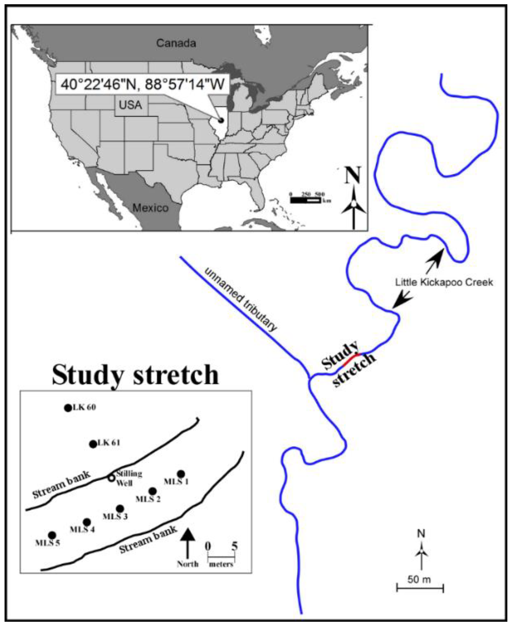
2.1. Site Description

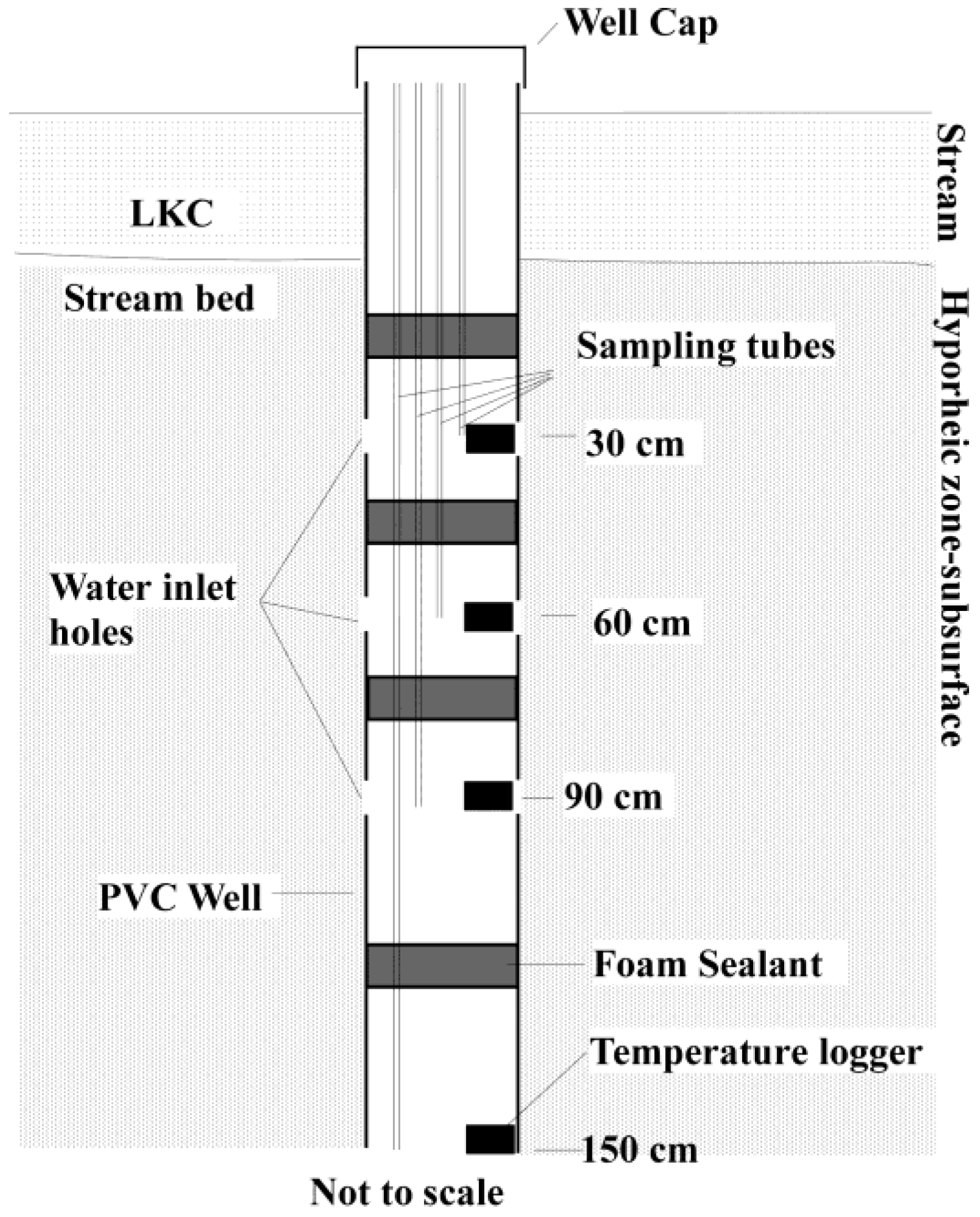
Fieldwork was conducted along a stretch of Little Kickapoo Creek (LKC) in central Illinois, USA (40°22′46″ N, 88°57′14″ W) (Figure 1). LKC is a third-order, low-gradient stream with a watershed that covers 76 km². Although the headwaters originate in an urban setting, land use is primarily agricultural, with corn and soybeans being the predominant crops [25].

The watershed is within the Bloomington Ridged Plain of the Till Plains Section, Central Lowland Province [53]. At the study location, three geologic units are relevant [51,54,55]. The Cahokia Alluvium, a 2-m thick Holocene floodplain deposit composed of sandy-silt, is the surficial unit. Underlying the Cahokia Alluvium is the Henry Formation, a glacial outwash deposited during the Wisconsinan Episode. The formation is 8 to 10 m of gravel with some coarse sand and serves as an aquifer. The Henry Formation is confined to a small valley that has been carved within the Tiskilwa Formation, a diamicton dominated by clay with some silt and fine sand.

The interface between the stream and the streambed occurs along the contact separating the Cahokia Alluvium and the Henry Formation; the gravels of the Henry Formation serve as the streambed [51,55]. A strong hydraulic connection between the stream and the underlying outwash aquifer has been documented [46,55,56,57,58]. Increases and decreases in the stream stage produced corresponding changes in the water level observed in wells within 50 m of the stream [55]. The water table in the area is located 1.5 to 2 m below the ground surface, and the regional hydraulic gradient is from the north to the south. Near LKC, the hydraulic gradient is toward the stream, with groundwater discharging into the stream [25,55,56,57,58]. Despite the observed upwelling of groundwater to LKC, a bromide tracer tests confirmed the downwelling of stream water to depths of 150 cm [59]. Although LKC has a low gradient (0.002) the streambed is mobile, with the top 30 cm of sediment entrained during bank full events on average every 7.6 months [51]. Limited vegetation has been observed along the streambed.

Stated NO₃-N concentrations in LKC water have ranged from below the detection limit to 9.7 mg/L. Lower NO₃-N concentrations are reported during late summer to fall, as compared to late winter to spring, when the highest NO₃-N concentrations are observed [25,46]. In the top 10 cm of the LKC streambed, denitrification and plant uptake have been reported as removal mechanisms for NO₃-N [60]. Other N species, ammonium, ammonia, nitrate, and dissolved organic nitrogen (DON), have been reported as non-detectable in the system [46] and were not examined for this work. As a conservative ion, Cl⁻ was analyzed to provide an understanding of the mixing within the system. Reported baseflow concentrations of Cl⁻ range from 60 to 90 mg/L; however, measured Cl⁻ concentrations following winter storm events can exceed 1700 mg/L [25,46]. The elevated Cl⁻ concentrations reflect the impact of road salts applied within the watershed [61,62,63].

2.2. Sampling

To measure seasonal changes in NO₃-N concentrations, 17 sample events were conducted from January 2012 to September 2012. At each event, stream water samples and streambed pore water samples were collected from five multi-level samplers installed along the thalweg of LKC (Figure 1). The multi-level samplers extend to a depth of 150 cm beneath the streambed surface with water intake at depths of 30 cm, 60 cm, 90 cm, and 150 cm below the streambed (Figure 2). To avoid the direct effects of scour, 30 cm was selected as the shallowest intake within the streambed. Separated by foam sealant, each intake zone was equipped with individual plastic tubing extending to the surface to allow for water extraction and a HOBO pendant recording water temperature every 15 min. Groundwater was collected from LK 60 and LK 61, which are water-table wells with screens extending to 2 m below the elevation of the stream-streambed interface. Hermit pressure transducers were installed in LK 60 and in the stilling well, recording the groundwater elevation and the stream stage at 15-min intervals, respectively.

From each zone within the multi-level samplers and the groundwater wells, water was pumped using a peristaltic pump while monitoring specific conductance (SpC) and temperature using a YSI-85 m (Yellow Springs Instrument Company, Inc., Yellow Springs, OH, USA). Upon parameter stabilization [64], the waters were filtered through a 0.45-mm filter and collected in acid-washed high-density polyethylene (HDPE) containers. While in the field and in transport, all samples were stored on ice; once at the laboratory, the samples were stored at 4 °C until being analyzed using a DIONEX ICS-1100 ion chromatography for chloride (Cl⁻) and nitrate as nitrogen (NO₃-N) measurements following the US Environmental Protection Agency method 300.1 [65]. Quality Assurance (QA) and quality control (QC) were maintained during the analysis of water samples by running blanks, duplicates, and replicates; the analytical error was less than 3%.

The presence of OM in sediments has been linked to nitrogen processing [66,67]. Employing the loss-on-ignition method [68], the OM within the streambed sediment at LKC was analyzed. Composite sediment samples of the top 25 cm of the streambed were collected adjacent to samplers 1, 3, and 5 once each month from May to October 2012. Samples were dried in an oven at 105 °C for 24 h to remove moisture, which was followed by four hours in a muffle furnace at 550 °C.

For each day of sampling, length of day data, to assess the photoperiod for vegetation, were collected from a weather station housed at the Central Illinois Regional Airport (KBMI), which is 10 km from the field site [69].

2.3. Mixing Model

A bromide tracer test illustrated the transport of bromide from the stream to a depth of 150 cm [59]. Within two hours after injection, bromide was observed at the 30-cm depth, highlighting the short lag time for the movement of water from the surface into the streambed. To determine the composition of the streambed pore water, a mixing model, where stream water and groundwater are the endmembers, was utilized. As a conservative tracer, Cl⁻ served as the parameter of interest to quantify the percentages of streambed pore water derived from stream water at the given depths using the formula [29,70]:

$$\%SW=\frac{\left(C{l}_{HZ}-C{l}_g\right)}{(C{l}_s-C{l}_g)}\text{×}100\%SW=\frac{\left(C{l}_{HZ}-C{l}_g\right)}{(C{l}_s-C{l}_g)}\text{×}100$$

(1)

where:

• %SW is the percentage of stream water within the streambed pore water (%),
• Cl_HZ is the chloride concentration in the streambed pore water at the depth of interest (mg/L),
• Cl_g is the chloride concentration in the groundwater (mg/L),
• Cl_s is the chloride concentration in the stream water (mg/L).

The composition of the water at the given depth determined from Equation (1) was employed to calculate the theoretical concentration of NO₃-N that should be present if mixing was the only potential control on concentration [71,72]. Assuming a conservative behavior for NO₃-N, with no denitrification, biotic uptake, or nitrification, and that the sources providing Cl⁻ are the same as those providing NO₃-N (surface water and groundwater, both lateral and vertical flow), the modeled concentration of NO₃-N present at a given depth was calculated using Equation (2):

$${\mathrm{NO}}_3\text{-}\mathrm{N}=\%SW*({\mathrm{N}}_{\mathrm{s}}-{\mathrm{N}}_{\mathrm{g}})+{\mathrm{N}}_{\mathrm{g}}{\mathrm{NO}}_3\text{-}\mathrm{N}=\%SW\ast \left({\mathrm{N}}_{\mathrm{s}}-{\mathrm{N}}_{\mathrm{g}}\right)+{\mathrm{N}}_{\mathrm{g}}$$

(2)

where:

• NO₃-N is the calculated concentration of NO₃-N in the pore water as a given depth (mg/L),
• N_s is the NO₃-N concentration of the stream water (mg/L),
• N_g is the NO₃-N concentration of the groundwater (mg/L).

The modeled values (Equation (2)) represent the NO₃-N concentrations if NO₃⁻ behaved conservatively. Deviations (ΔNO₃-N), either positive or negative, indicate the addition or removal of NO₃-N from the system, as compared to the conservative behavior of Cl⁻. The difference between the measured NO₃-N in the pore water and the modeled NO₃-N concentrations provided the ΔNO₃-N (mg/L).

$${\mathrm{NO}}_3\text{-}\mathrm{N}=\left({\mathrm{NO}}_3\text{-}\mathrm{N}\right){}_{\mathit{observed}}-\left({\mathrm{NO}}_3\text{-}\mathrm{N}\right){}_{\mathit{modeled}},\Delta {\mathrm{NO}}_3\text{-}\mathrm{N}={\left({\mathrm{NO}}_3\text{-}\mathrm{N}\right)}_{\mathit{observed}}-{\left({\mathrm{NO}}_3\text{-}\mathrm{N}\right)}_{\mathit{modeled}}$$

(3)

A positive ΔNO₃-N indicates that there is more NO₃-N present than what is expected based upon the mixing of surface water and groundwater, suggesting that nitrification has occurred. A negative ΔNO₃-N implies less NO₃-N in the waters than predicted based upon mixing; the ΔNO₃-N indicates the removal of NO₃-N, wither through microbial assimilation, plant uptake, or denitrification [73,74,75].

2.4. Statistical Analysis

A one-way analysis of variance (ANOVA) (α = 0.05) was used to determine if concentrations in waters at the different depths were statistically similar. Individual t-tests (α = 0.05) were used to assess if the stream water and the groundwater had different concentrations of NO₃-N and Cl⁻ to serve as endmembers of the mixing model. Linear relationships between ΔNO₃-N and the potential controlling variables—stream NO₃-N concentration, hydraulic gradient, OM, water temperature, and visible light—were determined examining the Pearson correlation coefficient and subsequently assigned a classification [76].

3. Results

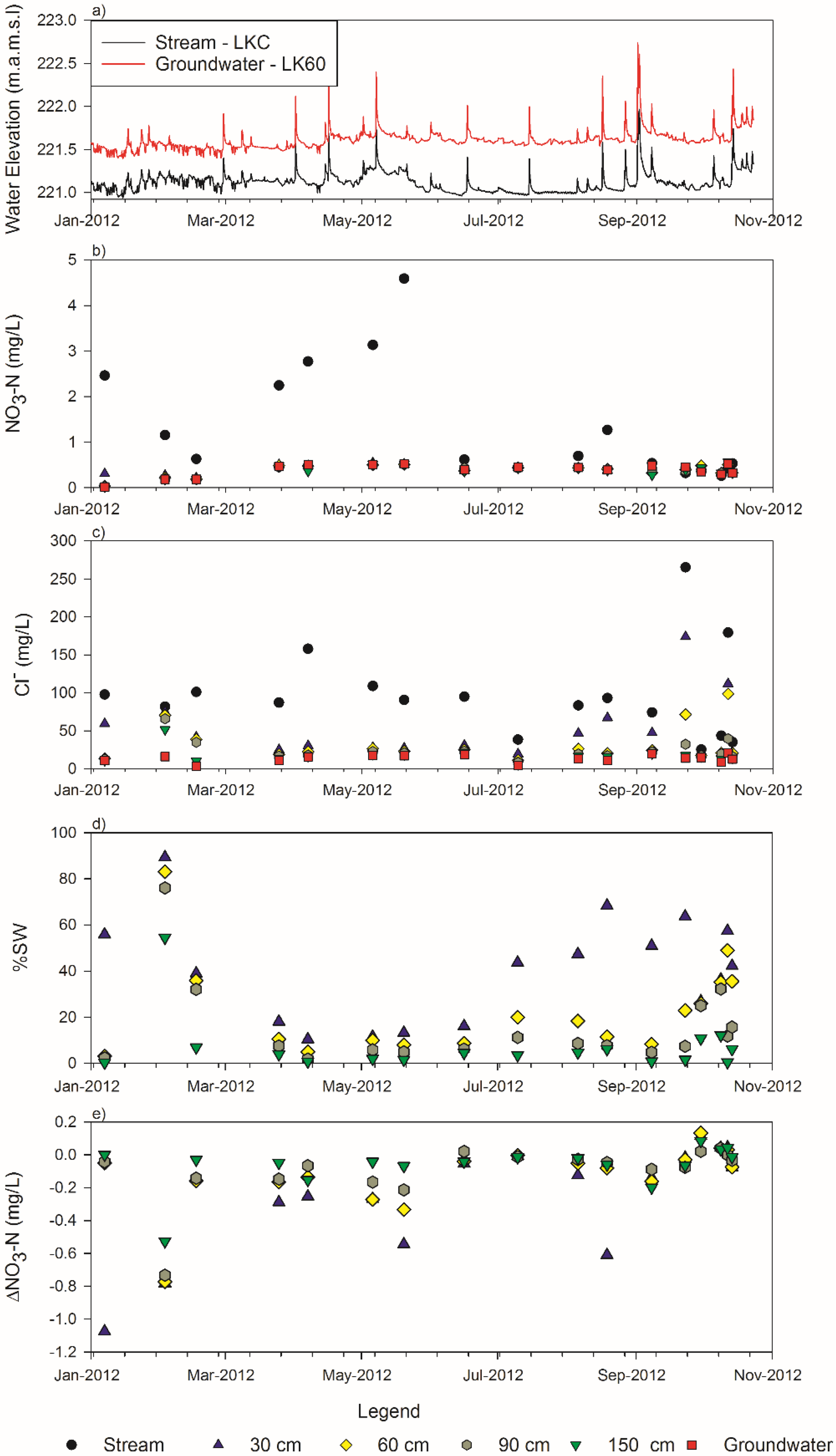
3.1. Stream and Groundwater

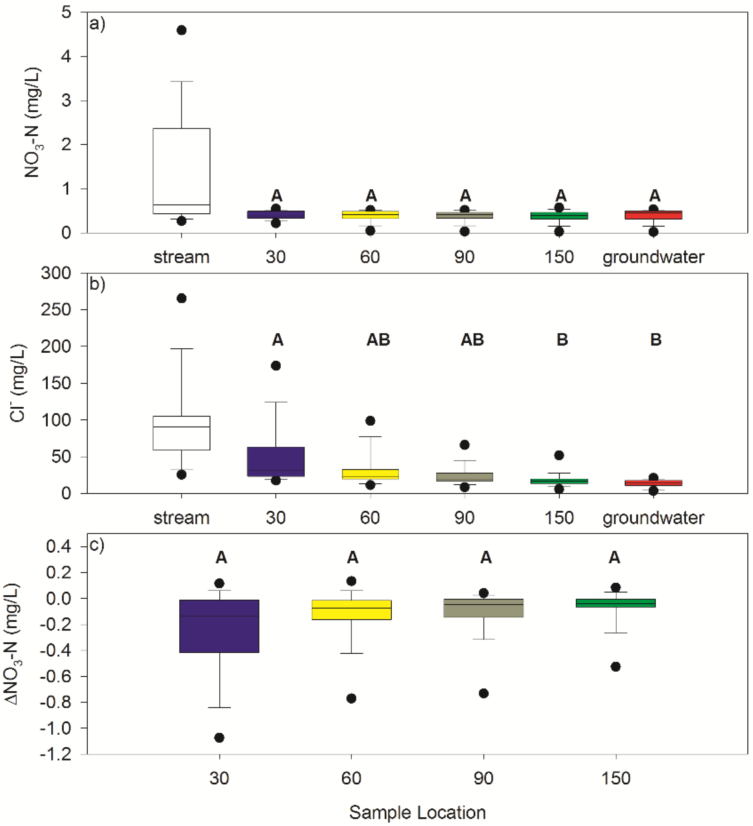
Stream flow in LKC varied during the sampling period. During winter and spring, LKC exhibited a higher mean stage at baseflow than during summer. As late summer and early fall precipitation events recharged the system, baseflow increased (Figure 3a). High-flow events occurred throughout the period, with larger magnitude events in April, May, and September. While mirroring the stage, the elevation of the groundwater was always higher than the stream stage. The mean hydraulic gradient between LK 60 and the stream was 0.029 m/m, providing a mean specific discharge from the groundwater to the stream of 2.9 × 10⁻⁶ m/s using the reported horizontal hydraulic conductivity (K) of 1.0 × 10⁻⁴ m/s [55,71]. From January to the end of May, the hydraulic gradient decreased as stream stage rose at a greater rate than the groundwater (Figure 4a). The largest hydraulic gradient, 0.035 m/m, was measured in June, coinciding with drier conditions and a lower stage. The hydraulic gradient was stable until September, when it started to decrease as the stage rose in response to recharge events.

3.2. Nitrate

NO₃-N concentrations of the stream water varied during the period (Figure 3b and

Table 1. Descriptive statistics of the seasonal nitrate as nitrogen and chloride concentration data for the water samples.

Sample Location	n	NO3-N (mg/L)			Cl− (mg/L)			ΔNO3-N (mg/L)
		Mean ± σ	Max	Min	Mean ± σ	Max	Min	Mean ± σ	Max	Min
Stream	17	1.32 ± 1.26	4.59	0.26	97.52 ± 58.80	265.29	25.36
30 cm	17	0.40 ± 0.09	0.54	0.21	49.64 ± 40.48	173.82	17.60	−0.25 ± 0.33	0.11	−1.08
60 cm	17	0.38 ± 0.13	0.51	0.04	32.83 ± 24.25	98.65	11.37	−0.13 ± 0.20	0.13	−0.77
90 cm	17	0.37 ± 0.13	0.51	0.03	24.00 ± 13.36	66.00	8.41	−0.10 ± 0.18	0.04	−0.73
150 cm	17	0.37 ± 0.14	0.57	0.02	17.89 ± 9.70	51.77	5.80	−0.07 ± 0.14	0.08	−0.53
Groundwater	34	0.38 ± 0.14	0.52	0.02	13.55 ± 4.93	21.06	3.49

), with a maximum concentration of 4.59 mg/L in May and concentrations less than 1 mg/L during summer and early fall. Higher concentrations were observed following periods of elevated stage following precipitation events, with lower concentrations during base flow. Similar concentration trends have been reported for LKC waters [25,46], indicating that the conditions during the observation period were consistent with those of other periods. NO₃-N concentration in the sediment pore waters and the groundwater were consistent across all of the depths over the entire period of time (Figure 3b and Table 1). The highest concentrations, above 0.50 mg/L, were measured in May; the lowest concentrations, less than 0.1 mg/L, were measured in January. A one-way ANOVA indicated that a statistical significant difference in NO₃-N concentrations exists among the depths/locations (F(5,96) = 8.955, p < 0.001) (Figure 5a). The t-tests indicated that the NO₃-N concentrations in the stream were different from the groundwater, establishing distinct endmembers for the mixing model.

3.3. Chloride

Chloride concentrations of the stream water varied throughout the period, following a different temporal trend from the NO₃-N (Figure 3c and Table 1). The maximum concentration of 265 mg/L and the minimum concentration of 25 mg/L were observed in September. Historically, the Cl⁻ concentrations illustrate temporal variability associated with the application of road salts [62,63]. The range of concentrations were consistent with previously reported values [25,46]. The trend of Cl⁻ concentrations within the streambed pore waters followed those in the stream, but the concentrations are lower (Figure 3c and Table 1). The Cl⁻ concentrations showed a consistent spatial trend where the shallower streambed depths had higher concentrations than the deeper levels, i.e., Cl⁻_stream > Cl⁻_30cm > Cl⁻_60cm > Cl⁻_90cm > Cl⁻_150cm > Cl⁻_groundwater (Figure 3c and Figure 5b). The concentrations were shown to be statistically different using a one-way ANOVA (F(5,96) = 16.702, p < 0.001). As with the NO₃-N, the t-tests confirmed that the stream Cl⁻ concentrations were different from those of the groundwater, establishing the two endmembers for the mixing model.

3.4. Mixing Model

The distribution of the Cl⁻ concentrations among the stream, the multi-level samplers, and the groundwater allowed the mixing model, Equations (1)–(3), to be used to determine the composition of the waters at a given depth (%SW) and to calculate the ΔNO₃-N, assuming no loss or removal of NO₃-N from the system. Downwelling of stream water was evident at all depths during the period of study (Figure 3d and

Table 2. Descriptive statistics of the calculated %SW ratios.

Sample Location	n	%SW
		Mean ± σ	Max	Min
30 cm	17	40% ± 22%	89%	11%
60 cm	17	83% ± 20%	83%	3%
90 cm	17	15% ± 18%	76%	2%
150 cm	34	7% ± 12%	54%	0%

). The 30-cm depth comprised the highest percentage of stream water, with a mean %SW of 41%, while at 150 cm the %SW was typically less than 10%. From April to July, the streambed waters exhibited the least amount of stream water across all depths, with the 30-cm depth exhibiting %SW from 10% to 18%; in the deeper waters, the %SW were all below 10%. Beginning in July, the percentage of stream water at the 30-cm depth rose; increases in the %SW ratios at the greater depths were observed to begin in September.

The reduction of NO₃-N, as indicated by negative ΔNO₃-N values, occurred from January through September at all depths within the streambed (Figure 3e and Table 1). The quantity of removal varied both spatially and temporally (Figure 3e). Spatially, the 30-cm depth exhibited the highest removal values (negative ΔNO₃-N values). The 150-cm depth exhibited the smallest removal values and the smallest variation. All depths exhibited a mean deficit, indicating the loss of NO₃-N, with the 30-cm depth having the largest deficit and exhibiting the greatest variance (Figure 5c). While visual inspection of the data indicated that the magnitude and variation of the mean deficit decreases with depth (Figure 5c), an ANOVA indicated that the values are not statistically different (F(3,67) = 2.108, p = 0.11).

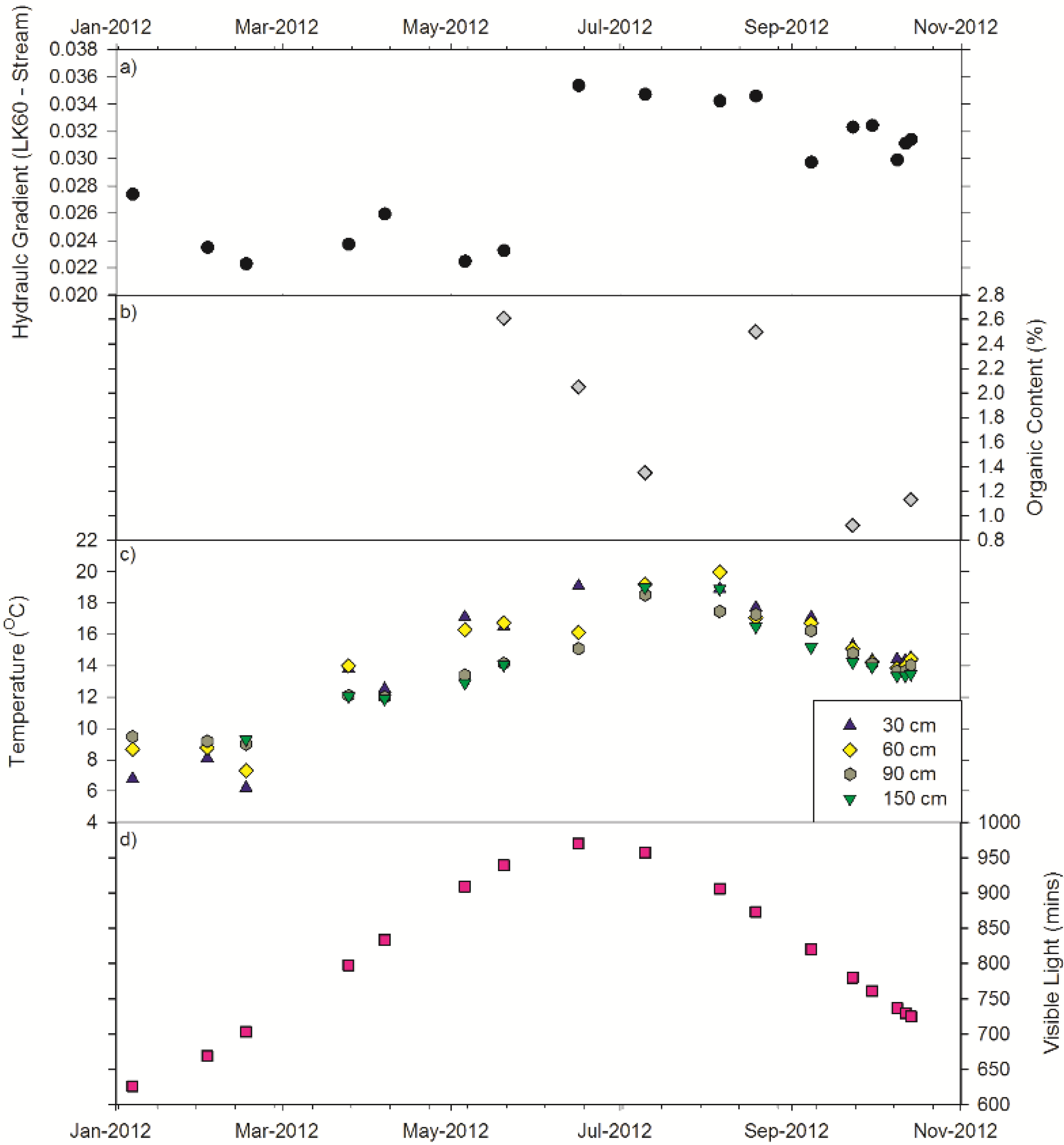
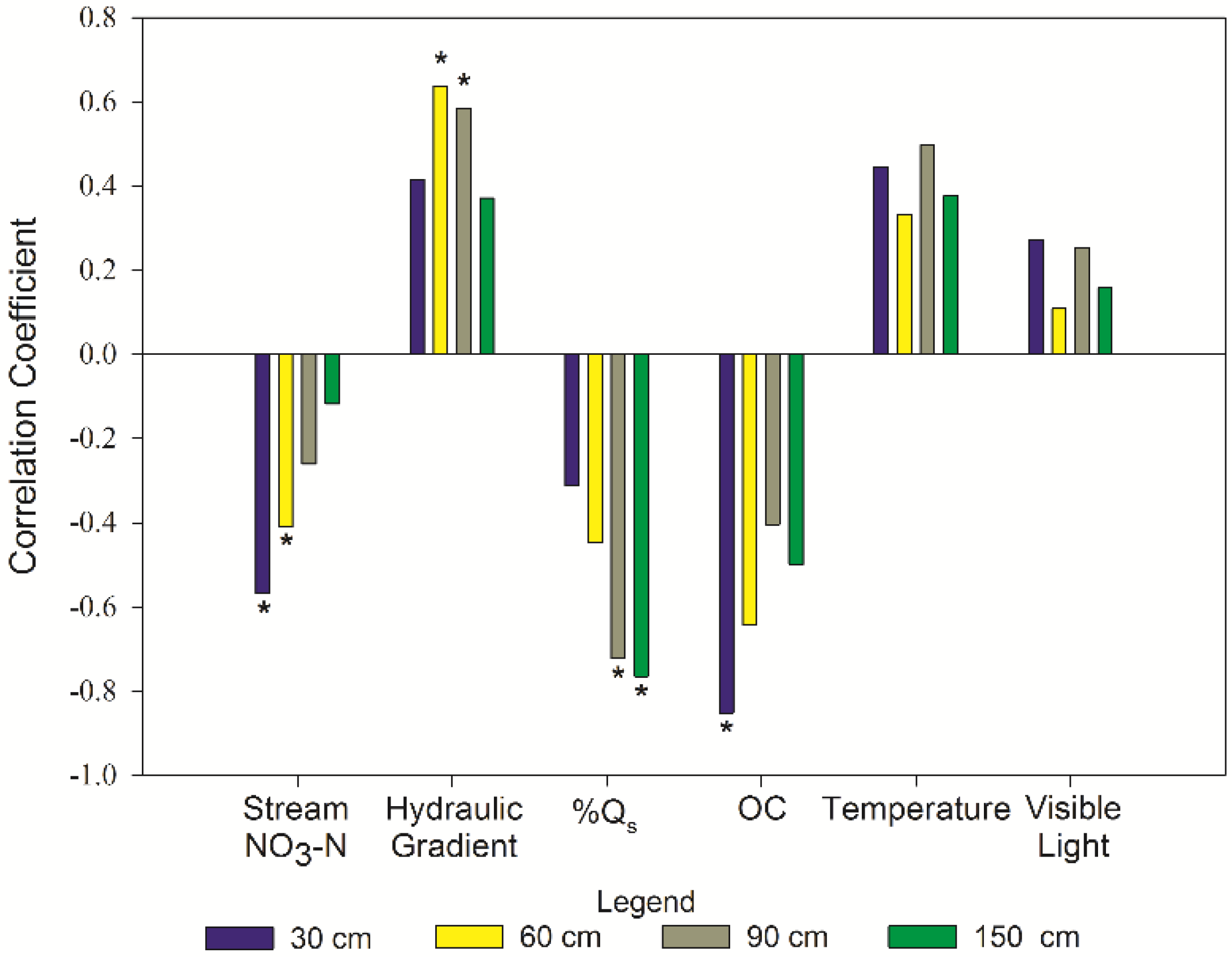
3.5. Controlling Factors

Sediment samples were taken once a month from May 2012 until October 2012 to observe changes in OM percent in the top 25 cm centimeters of the streambed (Figure 4b). The OM content was highest in May and decreased through July. An increase in OM was measured in August, when sampling was preceded by a recharge event less than 48 h prior. September and October exhibited depleted OM content similar to, but less than, those in July.

Temperatures within the hyporheic zone followed a sinusoidal trend increasing from the start of sampling in January until August/September, when temperatures started to decline (Figure 4c). The temperature followed a similar trend to the duration of visible light, but the peak temperature lagged the maximum measured visible light by two months (Figure 4d).

Pearson correlation analyses were conducted to assess the presence or absence of a correlation between the behavior of ΔNO₃-N and potential controlling factors. The potential controlling factors, including stream NO₃-N concentration; hydraulic gradient between LK 60 and the stream; %SW; the OM in the top 25 cm of the stream; water temperature; and visible light during a day, were compared to the ΔNO₃-N at each depth (Figure 6 and Figure 7). For %SW and water temperature, individual analyses comparing the ratio of %SW and the temperature at a given depth to the ΔNO₃-N at the same depth were completed, respectively. From the analyses, seven statistically significant correlations were identified (

Table 3. Pearson correlation results—statistically significant correlations.

Factors	N	r	p-Value	Classification 1
NO3-N stream: ΔNO3-N at 30 cm	17	−0.569	0.010	moderately negative
NO3-N stream: ΔNO3-N at 60 cm	17	−0.409	0.017	weakly negative
Hydraulic gradient: ΔNO3-N at 60 cm	17	0.636	<0.01	moderately positive
Hydraulic gradient: ΔNO3-N at 90 cm	17	0.584	0.01	moderately positive
%SW: ΔNO3-N at 150 cm	17	−0.765	<0.01	moderately negative
OM: ΔNO3-N at 30 cm	6	−0.852	0.031	strongly negative
%SW: ΔNO3-N at 90 cm	17	−0.723	<0.01	moderately negative

^1. Based upon Reference [76].

and Figure 7); no other statistically significant correlations were identified.

4. Discussion

While the magnitude varied, the hydraulic gradient indicated that groundwater flowed towards LKC, which was consistent with previous studies reporting LKC as a gaining stream [25,55,56,57,58]. Evidence of the upwelling of groundwater was observed in several instances while collecting water samples. After disconnecting the pump from the 150-cm sampling tubes, water continued to flow for a few seconds.

Regardless of whether a stream is gaining or losing water, downwelling into the streambed has been reported [77] and the mixing model quantified the mixing that has occurred (Figure 3d). Stream velocity and gradient influence the rate of downwelling [44,58,77]. At baseflow, when the stream stage is lower and the stream velocity is slower, downwelling stream water will compete against upwelling groundwater. Conversely, an elevated stage equates to a lower hydraulic gradient, increasing the potential for downwelling.

For LKC, the distribution of Cl⁻ concentrations across the depths highlighted the downwelling of stream water despite the upwelling of groundwater. Given the similarities in both the Cl⁻ and NO₃-N concentrations within the pore waters at 150 cm and the groundwater, the mixing model results revealed that the 150-cm depth was predominantly composed groundwater, with %SW amounting to less than 10%. With the exception of February, the waters at the 150-cm depth were comprised of less than 10% stream water. The amount of downwelling was temporally variable. From April to early July, evidence of downwelling was lacking. Only the 30-cm depth consistently had %SW values greater than 10%. Corresponding to the lower hydraulic gradient observed in winter and spring, the mixing model data signaled that the stream water was transported to a depth between 90 and 150 cm. During summer and fall, when a greater hydraulic gradient was present, the mixing model results showed that waters at 90 cm contained less than 10% stream water, suggesting that upwelling limited the penetration depth of the stream water. The thinner mixing area in summer and fall coincided with the greater potential for groundwater upwelling (higher hydraulic gradient) and the thicker mixing area occurred during the period of low hydraulic gradient.

The measured NO₃-N concentrations in the stream water were consistent with previously reported concentrations observed in LKC. Similar to trends reported by References [25,46], the highest measured concentrations occurred in spring and early summer, while the lowest concentrations were in late summer and early fall. Nitrate concentrations in the stream rapidly decreased from a peak of 4.59 mg/L at the beginning of May to 0.62 mg/L in June, where concentrations remained for the duration of the study. With the exception of early fall, higher NO₃-N concentrations were measured in the stream water than the groundwater, with the contrast between the means (1.32 mg/L and 0.38 mg/L, respectively) highlighting the difference. Exhibiting little variation, the NO₃-N concentrations of the streambed pore waters were similar to those of the groundwater (Figure 5a).

Assuming only mixing and the strong potential for groundwater upwelling into the stream, similar NO₃-N concentrations among the depths and groundwater was expected. However, the distribution of Cl⁻ concentrations with depth supported the occurrence of downwelling stream water. Differences in NO₃-N concentrations at the depths cannot be accounted for solely by the mixing ratios generated with the Cl⁻ concentrations; that is, the ΔNO₃-N values were not 0 mg/L. From January to September, the sediment pore waters produced negative ΔNO₃-N values, indicating a depletion or loss of nitrate from the system. The majority of the nitrate loss occurred in the top 30 cm, with a mean reduction of 0.25 mg/L, which represents 19% of the stream water concentration. Progressing deeper into the sediment, removal rates (negative ΔNO₃-N) slowed. At 150 cm, the loss of nitrate continued, but negative ΔNO₃-N values approach 0 mg/L (less removal). References [66,78] reported that while denitrification rates were highest in the top 5 cm, denitrification continued to a depth of at least 25 cm, the deepest point of measurement. Our results suggest that NO₃-N removal continues to a depth of 150 cm.

A lower hydraulic gradient allows for easier downwelling, resulting in longer residence times (less potential to return to the stream). Residing in the streambed for longer periods of time leads to greater denitrification as a result of enhanced opportunity for biogeochemical processing [36,44,79]. While residence time was not measured, %SW values, a proxy of travel distance and time, suggest longer residence times in winter and late summer to early fall. As downwelling transported water deeper into the substrate, the removal of NO₃-N was observed. However, the calculated ΔNO₃-N values do not suggest a consistent relationship between residence time and NO₃-N removal. The largest negative ΔNO₃-N values occurred in winter, corresponding to greater infiltration depths of stream water flux. In late summer to early fall, less removal occurred, although stream water penetrated a similar depth to that observed in winter. The difference between these periods is the stream NO₃-N concentration, which is higher in winter and lower in summer. While fluid flux plays a role, if the supply of nitrate is limited, removal is constrained [6,42,43,78,80,81,82,83].

The trend of ΔNO₃-N values mimicked the concentrations of NO₃-N in the stream, which was confirmed by the significant negative correlations observed at the 30-cm and 60-cm depths. At lower stream NO₃-N concentrations (less than 0.4 mg/L) the ΔNO₃-N values were slightly positive (Figure 6a), indicating the addition of NO₃-N to the system. As stream NO₃-N concentrations increased, the ΔNO₃-N values approached zero (0), and then became deficient in NO₃-N (negative ΔNO₃-N values), suggesting that NO₃-N was being removed within the streambed. The larger negative ΔNO₃-N values were attributed to the downwelling of stream water with higher NO₃-N concentrations into the streambed. Plant uptake, microbial assimilation, and denitrification were potential pathways for NO₃-N removal [84,85,86,87]. Seasonal changes in solar radiation influence the growth of aquatic plants and algae by controlling photosynthesis [7,43,66]. While photosynthesis creates a complex set of interactions, the highest rates of plant and algal NO₃-assimilation are reported during periods of greater sunlight [88,89]. The absence of a correlation between ΔNO₃-N values and visible light at all depths suggest that photosynthesis is not a direct factor controlling NO₃-N removal (Figure 7). The negligible vegetation along the streambed coupled with no relationship to sunlight indicate that plant uptake was a minimal pathway for NO₃-N removal.

In similar systems, denitrification has been identified as the dominant mechanism of NO₃-N removal [35,40,42,43]. Also, in LKC, Reference [60] documented the reduction of NO₃-N via denitrification and plant uptake within the top 10 cm of the LKC streambed. This work did not conduct a direct measurement of removal processes; however, the data suggest denitrification was the primary mechanism. Sediments in the agricultural streams of Illinois are capable of supporting high rates of denitrification for much of the year [45], implying a removal mechanism throughout the year. Studies have shown that elevated concentrations of organic matter in the streambed can stimulate denitrification within the streambed when NO₃-N concentrations in the stream system are high [6,66,67,78,82]. The strong negative correlation observed between OM and ΔNO₃-N at a depth of 30 cm demonstrates the importance of OM to the removal of NO₃-N. The lack of correlation at greater depths does not discount the role of OM on the process but may speak to the supply of OM at those depths. The top 30 cm of the LKC streambed is entrained and redistributed on average every eight months [51]. As sediment is deposited, OM is also incorporated, replenishing the supply for continued denitrification [33,38]. As the sediment is more stable at deeper levels, the OM is expected to be lower (depleted) and not easily replenished. Thus, the OM at a depth of 30 cm would not be representative of conditions at deeper levels.

5. Conclusions

The results of this study support the hypothesis that nitrate loss occurs at depths below 25 cm. Concentrations of NO₃-N in the pore waters at the given depths were lower than those measured in the stream waters, which was expected given the mixing of upwelling groundwater that had low NO₃-N concentrations with downwelling stream water that had higher concentrations. The mixing models generated ΔNO₃-N values that indicated deficits of NO₃-N at all of the depths. At the 30-cm depth, the mean ΔNO₃-N of −0.25 mg/L identified a deficit (loss) of NO₃-N as compared to the expected concentration (assuming that only mixing occurred). Calculated negative ΔNO₃-N values show that the removal of NO₃-N occurred to depths of 150 cm, which extends the depth beyond 25 cm reported by References [66,78]. However, the amount of removal was not spatially or temporally consistent. Larger negative ΔNO₃-N values were calculated for the 30-cm depth, representing more NO₃-N removal. Traveling deeper into the streambed, the negative ΔNO₃-N values approached zero, indicating less NO₃-N removal. Nearer the surface (30 cm and 60 cm), the removal of NO₃-N (ΔNO₃-N) was correlated to stream NO₃-N concentrations and OM. Deeper in the substrate (90 cm and 150 cm), water movement, as calculated by both hydraulic gradient and %SW, was a more controlling factor. No correlation between ΔNO₃-N and visible light nor temperature was observed. The supply of NO₃-N appeared to be the primary control; when stream NO₃-N concentrations were lowest, the lowest rates of removal were observed.

In LKC, NO₃-N removal rates were low—approaching zero in June and August when visible light and, subsequently, plant uptake would be optimal. The highest removal rates occurred in January and February, when plants were dormant. During the study, the streambed lacked significant vegetation. Thus, the absence of plant uptake suggests that denitrification was the main mechanism of NO₃-N removal. As mentioned, a significant limitation to this work is the absence of the direct measurement of denitrification or nitrification. The work essentially accounts for net nitrogen activity. Without a direct measurement of the processes, the interpretations are limited to relationships between NO₃-N removal/addition and the controlling variables. To elucidate the primary factors and to confirm the results of other studies, additional work is needed. Given that denitrification was not directly measured, this work cannot confirm denitrification at depths greater than 25 cm [66], but the observation of negative ΔNO₃-N values corroborates nitrate removal at depths greater than 30 cm in streambeds.

References

1. Oberle, S.L.; Keeney, D.R. Factors influencing corn fertilizer N requirements in the northern US corn belt. J. Prod. Agric. 1990, 3, 527–534. [Google Scholar] [CrossRef]
2. Gentry, L.E.; David, M.B.; Smith, K.M.; Kovacic, D.A. Nitrogen cycling and tile drainage nitrate loss in a corn/soybean watershed. Agric. Ecosyst. Environ. 1998, 68, 85–97. [Google Scholar] [CrossRef]
3. Alexander, R.B.; Boyer, E.W.; Smith, R.A.; Schwarz, G.E.; Moore, R.B. The Role of headwater streams in downstream water quality. J. Am. Water Resour. Assoc. 2007, 43, 41–59. [Google Scholar] [CrossRef] [PubMed]
4. Dagg, M.J.; Breed, G.A. Biological effects of Mississippi River nitrogen on the northern gulf of Mexico—A review and synthesis. J. Mar. Syst. 2003, 43, 133–152. [Google Scholar] [CrossRef]
5. Scavia, D.; Justic, D.; Bierman, V.J.J. Reducing hypoxia in the Gulf of Mexico: Advice from three models. Estuaries 2004, 27, 419–425. [Google Scholar] [CrossRef]
6. Arango, C.P.; Tank, J.L.; Schaller, J.L.; Royer, T.V.; Bernot, M.J.; David, M.B. Benthic organic carbon influences denitrification in streams with high nitrate concentration. Freshw. Biol. 2007, 52, 1210–1222. [Google Scholar] [CrossRef] [Green Version]
7. Christensen, P.B.; Nielsen, L.P.; Sorensen, J.; Revsbech, N.P. Denitrification in nitrate-rich streams: Diurnal and seasonal variation related to benthic oxygen metabolism. Limnol. Oceanogr. 1990, 35, 640–651. [Google Scholar] [CrossRef] [Green Version]
8. Goolsby, D.A.; Battaglin, W.A.; Aulenbach, B.T.; Hooper, R.P. Nitrogen input to the Gulf of Mexico. J. Environ. Qual. 2001, 30, 329–336. [Google Scholar] [CrossRef] [PubMed]
9. Scavia, D.; Rabalais, N.N.; Turner, R.E.; Justić, D.; Wiseman, W.J., Jr. Predicting the response of Gulf of Mexico hypoxia to variations in Mississippi River nitrogen load. Limnol. Oceanogr. 2003, 48, 951–956. [Google Scholar] [CrossRef]
10. Scott, D.; Harvey, J.; Alexander, R.; Schwarz, G. Dominance of organic nitrogen from headwater streams to large rivers across the conterminous United States. Glob. Biogeochem. Cycles 2007, 21, GB1003. [Google Scholar] [CrossRef]
11. Boulton, A.J.; Findlay, S.; Marmonier, P. The functional significance of the hyporheic zone in streams and rivers (review). Ann. Rev. Ecol. Syst. 1998, 29, 59–81. [Google Scholar] [CrossRef]
12. David, M.B.; Wall, L.G.; Royer, T.V.; Tank, J.L. Denitrification and the nitrogen budget of a reservoir in an agricultural landscape. Ecol. Appl. 2006, 16, 2177–2190. [Google Scholar] [CrossRef]
13. Keeney, D.R.; Hatfield, J.L. The nitrogen cycle: Historical perspective, and current and potential future concerns. In Nitrogen in the Environment: Sources, Problems, and Solutions; Follett, R., Hatfield, J.L., Eds.; Elsevier: Amsterdam, The Netherlands, 2001; pp. 3–16. [Google Scholar]
14. Rabalais, N.; Turner, R.E.; Dortch, Q.; Justic, D.; Bierman, V., Jr.; Wiseman, W., Jr. Nutrient-enhanced productivity in the northern Gulf of Mexico: Past, present and future. In Nutrients and Eutrophication in Estuaries and Coastal Waters; Orive, E., Elliott, M., de Jonge, V., Eds.; Springer: Dordrecht, The Netherlands, 2002; Volume 164, pp. 39–63. [Google Scholar]
15. Turner, R.E.; Rabalais, N.N.; Justic, D. Predicting summer hypoxia in the northern Gulf of Mexico: Riverine N, P, and Si loading. Mar. Pollut. Bull. 2006, 52, 139–148. [Google Scholar] [CrossRef] [PubMed]
16. Turner, R.E.; Rabalais, N.N.; Justić, D. Predicting summer hypoxia in the northern Gulf of Mexico: Redux. Mar. Pollut. Bull. 2012, 64, 319–324. [Google Scholar] [CrossRef] [PubMed]
17. Hashemi, F.; Olesen, J.E.; Hansen, A.L.; Børgesen, C.D.; Dalgaard, T. Spatially differentiated strategies for reducing nitrate loads from agriculture in two Danish catchments. J. Environ. Manag. 2018, 208, 77–91. [Google Scholar] [CrossRef] [PubMed]
18. Sharma, L.K.; Bali, S.K. A review of methods to improve nitrogen use efficiency in agriculture. Sustainability 2018, 10. [Google Scholar] [CrossRef]
19. Sieczka, A.; Koda, E. Kinetic and Equilibrium Studies of Sorption of Ammonium in the Soil-Water Environment in Agricultural Areas of Central Poland. Appl. Sci. 2016, 6, 269. [Google Scholar] [CrossRef]
20. David, M.B.; Gentry, L.E. Anthropogenic inputs of nitrogen and phosphorus and riverine export for Illinois, USA. J. Environ. Qual. 2000, 29, 494–508. [Google Scholar] [CrossRef]
21. Delgado, J.A. Quantifying the loss mechanisms of nitrogen. J. Soil Water Conserv. 2002, 57, 389–398. [Google Scholar]
22. Follett, R.F.; Delgado, J.A. Nitrogen fate and transport in agricultural systems. J. Soil Water Conserv. 2002, 57, 402–408. [Google Scholar]
23. Kovacic, D.A.; David, M.B.; Gentry, L.E.; Starks, K.M.; Cooke, R.A. Effectiveness of constructed wetlands in reducing nitrogen and phosphorus export from agricultural tile drainage. J. Environ. Qual. 2000, 29, 1262–1274. [Google Scholar] [CrossRef]
24. Mehnert, E.; Hwang, H.-H.; Johnson, T.M.; Sanford, R.A.; Beaumont, W.C.; Holm, T.R. Denitrification in the shallow ground water of a tile-drained, agricultural watershed. J. Environ. Qual. 2007, 36, 80–90. [Google Scholar] [CrossRef] [PubMed]
25. Peterson, E.W.; Benning, C. Factors influencing nitrate within a low-gradient agricultural stream. Environ. Earth Sci. 2013, 68, 1233–1245. [Google Scholar] [CrossRef]
26. Schilling, K.; Zhang, Y.-K. Baseflow contribution to nitrate-nitrogen export from a large, agricultural watershed, USA. J. Hydrol. 2004, 295, 305–316. [Google Scholar] [CrossRef]
27. Bardini, L.; Boano, F.; Cardenas, M.B.; Revelli, R.; Ridolfi, L. Nutrient cycling in bedform induced hyporheic zones. Geochim. Cosmochim. Acta 2012, 84, 47–61. [Google Scholar] [CrossRef] [Green Version]
28. Duff, J.H.; Triska, F.J. Denitrification in sediments from the hyporheic zone adjacent to a small forested stream. Can. J. Fish. Aquat. Sci. 1990, 47, 1140–1147. [Google Scholar] [CrossRef]
29. Triska, F.J.; Kennedy, V.C.; Avanzino, R.J.; Zellweger, G.W.; Bencala, K.E. Retention and transport of nutrients in a third-order stream in northwestern California: Hyporheic processes. Ecology 1989, 70, 1893–1905. [Google Scholar] [CrossRef]
30. Zarnetske, J.P.; Haggerty, R.; Wondzell, S.M.; Bokil, V.A.; Gonzalez-Pinzon, R. Coupled transport and reaction kinetics control the nitrate source-sink function of hyporheic zones. Water Resour. Res. 2012, 48, 15. [Google Scholar] [CrossRef]
31. Storey, R.G.; Williams, D.D.; Fulthorpe, R.R. Nitrogen processing in the hyporheic zone of a pastoral stream. Biogeochemistry 2004, 69, 285–313. [Google Scholar] [CrossRef]
32. Hinkle, S.R.; Duff, J.H.; Triska, F.J.; Laenen, A.; Gates, E.B.; Bencala, K.E.; Wentz, D.A.; Silva, S.R. Linking hyporheic flow and nitrogen cycling near the Willamette River—A large river in Oregon, USA. J. Hydrol. 2001, 244, 157–180. [Google Scholar] [CrossRef]
33. Hill, A.R.; Labadia, C.F.; Sanmugadas, K. Hyporheic zone hydrology and nitrogen dynamics in relation to the streambed topography of a N-rich stream. Biogeochemistry 1998, 42, 285–310. [Google Scholar] [CrossRef]
34. Findlay, S.; Strayer, D.; Goumbala, C.; Gould, K. Metabolism of streamwater dissolved organic carbon in the shallow hyporheic zone. Limnol. Oceanogr. 1993, 38, 1493–1499. [Google Scholar] [CrossRef] [Green Version]
35. Fischer, H.; Kloep, F.; Wilzcek, S.; Pusch, M.T. A river’s liver—Microbial processes within the hyporheic zone of a large lowland river. Biogeochemistry 2005, 76, 349–371. [Google Scholar] [CrossRef]
36. Opdyke, M.R.; David, M.B.; Rhoads, B.L. Influence of geomorphological variability in channel characteristics on sediment denitrification in agricultural streams. J. Environ. Qual. 2006, 35, 2103–2112. [Google Scholar] [CrossRef] [PubMed]
37. Peterson, B.J.; Wollheim, W.M.; Mulholland, P.J.; Webster, J.R.; Meyer, J.L.; Tank, J.L.; Martí, E.; Bowden, W.B.; Valett, H.M.; Hershey, A.E.; et al. Control of nitrogen export from watersheds by headwater streams. Science 2001, 292, 86–90. [Google Scholar] [CrossRef] [PubMed]
38. Pind, A.; Risgaard-Petersen, N.; Revsbech, N.P. Denitrification and microphytobenthic NO3 consumption in a Danish lowland stream: Diurnal and seasonal variation. Aquat. Microb. Ecol. 1997, 12, 275–284. [Google Scholar] [CrossRef]
39. Brunke, M.; Gonser, T. The ecological significance of exchange processes between rivers and groundwater. Freshw. Biol. 1997, 37, 1–33. [Google Scholar] [CrossRef] [Green Version]
40. Gu, C.; Hornberger, G.M.; Mills, A.L.; Herman, J.S.; Flewelling, S.A. Nitrate reduction in streambed sediments: Effects of flow and biogeochemical kinetics. Water Resour. Res. 2007, 43. [Google Scholar] [CrossRef] [Green Version]
41. Kemp, M.J.; Dodds, W.K. Comparisons of nitrification and denitrification in prairie and agriculturally influenced streams. Ecol. Soc. Am. 2002, 12, 998–1009. [Google Scholar] [CrossRef]
42. Mulholland, P.J.; Helton, A.M.; Poole, G.C.; Hall, R.O.; Hamilton, S.K.; Peterson, B.J.; Tank, J.L.; Ashkenas, L.R.; Cooper, L.W.; Dahm, C.N.; et al. Stream denitrification across biomes and its response to anthropogenic nitrate loading. Nature 2008, 452, 202–205. [Google Scholar] [CrossRef] [PubMed] [Green Version]
43. O’Brien, J.M.; Dodds, W.K.; Wilson, K.C.; Murdock, J.N.; Eichmiller, J. Saturation of N cycling in Central Plains streams: 15N experiments across a broad gradient of nitrate concentrations. Biogeochemistry 2007, 84, 31–49. [Google Scholar] [CrossRef]
44. Zarnetske, J.P.; Haggerty, R.; Wondzell, S.M.; Baker, M.A. Dynamics of nitrate production and removal as a function of residence time in the hyporheic zone. J. Geophys. Res. Biogeosci. 2011, 116, G01025. [Google Scholar] [CrossRef]
45. Royer, T.V.; Tank, J.L.; David, M.B. Transport and fate of nitrate in headwater agricultural streams in Illinois. J. Environ. Qual. 2004, 33, 1296–1304. [Google Scholar] [CrossRef] [PubMed]
46. Van der Hoven, S.J.; Fromm, N.J.; Peterson, E.W. Quantifying nitrogen cycling beneath a meander of a low gradient, N-impacted, agricultural stream using tracers and numerical modelling. Hydrol. Proc. 2008, 22, 1206–1215. [Google Scholar] [CrossRef]
47. Chavan, P.V.; Dennett, K.E.; Marchand, E.A.; Spurkland, L.E. Potential of constructed wetland in reducing total nitrogen loading into the Truckee River. Wetl. Ecol. Manag. 2008, 16, 189–197. [Google Scholar] [CrossRef]
48. Wollheim, W.M.; Harms, T.K.; Peterson, B.J.; Morkeski, K.; Hopkinson, C.S.; Stewart, R.J.; Gooseff, M.N.; Briggs, M.A. Nitrate uptake dynamics of surface transient storage in stream channels and fluvial wetlands. Biogeochemistry 2014, 120, 239–257. [Google Scholar] [CrossRef]
49. Alexander, R.B.; Smith, R.A.; Schwarz, G.E. Effect of stream channel size on the delivery of nitrogen to the Gulf of Mexico. Nature 2000, 403, 758–761. [Google Scholar] [CrossRef] [PubMed]
50. Kasahara, T.; Hill, A.R. Lateral hyporheic zone chemistry in an artificially constructed gravel bar and a re-meandered stream channel, southern Ontario, Canada. J. Am. Water Resour. Assoc. 2007, 43, 1257–1269. [Google Scholar] [CrossRef]
51. Peterson, E.W.; Sickbert, T.B.; Moore, S.L. High frequency stream bed mobility of a low-gradient agricultural stream with implications on the hyporheic zone. Hydrol. Process. 2008, 22, 4239–4248. [Google Scholar] [CrossRef]
52. Goodale, C.L.; Aber, J.D.; Vitousek, P.M.; McDowell, W.H. Long-term decreases in stream nitrate: Successional causes unlikely; Possible links to DOC? Ecosystem 2005, 8, 334–337. [Google Scholar] [CrossRef]
53. Illinois State Geological Survey. Physiographic Division of Illinois. Available online: http://isgs.illinois.edu/sites/isgs/files/maps/statewide/physio-w-color-8x11.pdf (accessed on 8 March 2018).
54. Ludwikowski, J.; Malone, D.H.; Peterson, E.W. Surficial geologic map, Bloomington East Quadrangle, McLean County, Illinois. Available online: http://isgs.illinois.edu/maps/isgs-quads/surficial-geology/student-map/bloomington-east (accessed on 8 March 2018).
55. Peterson, E.W.; Sickbert, T.B. Stream water bypass through a meander neck, laterally extending the hyporheic zone. Hydrogeol. J. 2006, 14, 1443–1451. [Google Scholar] [CrossRef]
56. Bastola, H.; Peterson, E.W. Heat tracing to examine seasonal groundwater flow beneath a low-gradient stream. Hydrogeol. J. 2016, 24, 181–194. [Google Scholar] [CrossRef]
57. Beach, V.; Peterson, E.W. Variation of hyporheic temperature profiles in a low gradient third-order agricultural stream—A statistical approach. Open J. Modern Hydrol. 2013, 3, 55–66. [Google Scholar] [CrossRef]
58. Sickbert, T.B.; Peterson, E.W. The effect of surface water velocity on hyporheic interchange. J. Water Resour. Prot. 2014, 6, 327–336. [Google Scholar] [CrossRef]
59. Bastola, H. Identifying Seasonal Changes in Streambed Thermal Profile in a Third Order Agricultural Stream using 2D Thermal Modeling. Master’s Thesis, Illinois State University, Normal, IL, USA, 2011. [Google Scholar]
60. Buyck, M.S. Tracking Nitrate Loss and Modeling Flow through the Hyporheic Zone of a Low Gradient Stream through the Use of Conservative Tracers. Master’s Thesis, Illinois State University, Normal, IL, USA, 2005. [Google Scholar]
61. Lax, S.; Peterson, E.W. Characterization of chloride transport in the unsaturated zone near salted road. Environ. Geol. 2009, 58, 1041–1049. [Google Scholar] [CrossRef]
62. Lax, S.M.; Peterson, E.W.; Van der Hoven, S. Quantifying Stream chloride concentrations as a function of land-use. Environ. Earth Sci. 2017, 76, 12. [Google Scholar] [CrossRef]
63. Ludwikowski, J.J.; Peterson, E.W. Transport and fate of chloride from road salt within a mixed urban and agricultural watershed in Illinois (USA): Assessing the influence of chloride application rates. Hydrogeol. J. 2018. [Google Scholar] [CrossRef]
64. Barcelona, M.J.; Gibb, J.P.; Helfrich, J.A.; Garske, E.E. Practical Guide for Ground-Water Sampling; Illinois State Water Survey, Ed.; Illinois State Water Survey: Champaign, IL, USA, 1985; Volume ISWS CR-374, p. 94. [Google Scholar]
65. Hautman, D.P.; Munch, D.J.J.E.O. Method 300.1: Determination of Inorganic Anions in Drinking Water by Ion Chromatography; U.S. Environmental Protection Agency: Cincinnati, OH, USA, 1997.
66. Stelzer, R.S.; Bartsch, L.A.; Richardson, W.B.; Strauss, E.A. The dark side of the hyporheic zone: Depth profiles of nitrogen and its processing in stream sediments. Freshw. Biol. 2011, 56, 2021–2033. [Google Scholar] [CrossRef]
67. Stelzer, R.S.; Thad Scott, J.; Bartsch, L.A.; Parr, T.B. Particulate organic matter quality influences nitrate retention and denitrification in stream sediments: Evidence from a carbon burial experiment. Biogeochemistry 2014, 119, 387–402. [Google Scholar] [CrossRef]
68. Schulte, E.E.; Hopkins, B.G. Estimation of soil organic matter by weight loss-on-ignition. In Soil Organic Matter: Analysis and Interpretation; Magdoff, F.R., Tabatabia, M.A., Hanlon, E.A., Eds.; Soil Science Society of America: Madison, WI, USA, 1996; pp. 21–31. [Google Scholar]
69. Weather Underground. Weather History for KBMI. Available online: https://www.wunderground.com/history/airport/KBMI/ (accessed on 6 March 2017).
70. Hill, A.R.; Lymburner, D.J. Hyporheic zone chemistry and stream-subsurface exchange in two groundwater-fed streams. Can. J. Fish. Aquat. Sci. 1998, 55, 495–506. [Google Scholar] [CrossRef]
71. Ackerman, J.R.; Peterson, E.W.; Van der Hoven, S.; Perry, W. Quantifying nutrient removal from groundwater seepage out of constructed wetlands receiving treated wastewater effluent. Environ. Earth Sci. 2015, 74, 1633–1645. [Google Scholar] [CrossRef]
72. Maxwell, E.L.; Peterson, E.W.; O’Reilly, C.M. Enhanced nitrate reduction within a constructed wetland system: Nitrate removal within groundwater flow. Wetlands 2017, 37, 413–422. [Google Scholar] [CrossRef]
73. Jaynes, D.B.; Isenhart, T.M. Reconnecting tile drainage to riparian buffer hydrology for enhanced nitrate removal. J. Environ. Qual. 2014, 43, 631–638. [Google Scholar] [CrossRef] [PubMed]
74. Kuusemets, V.; Mander, Ü.; Lõhmus, K.; Ivask, M. Nitrogen and phosphorus variation in shallow groundwater and assimilation in plants in complex riparian buffer zones. Water Sci. Technol. 2001, 44, 615–622. [Google Scholar] [CrossRef] [PubMed]
75. Zumft, W.G. Cell biology and molecular basis of denitrification. Microbiol. Mol. Biol. Rev. 1997, 61, 533–616. [Google Scholar] [PubMed]
76. Zou, K.H.; Tuncali, K.; Silverman, S.G. Correlation and simple linear regression. Radiology 2003, 227, 617–628. [Google Scholar] [CrossRef] [PubMed]
77. Fox, A.; Boano, F.; Arnon, S. Impact of losing and gaining streamflow conditions on hyporheic exchange fluxes induced by dune-shaped bed forms. Water Resour. Res. 2014, 50, 1895–1907. [Google Scholar] [CrossRef] [Green Version]
78. Inwood, S.E.; Tank, J.L.; Bernot, M.J. Factors controlling sediment denitrification in midwestern streams of varying land use. Microb. Ecol. 2007, 53, 247–258. [Google Scholar] [CrossRef] [PubMed]
79. Runkel, R.L. Toward a transport-based analysis of nutrient spiraling and uptake in streams. Limnol. Oceanogr. Methods 2007, 5, 50–62. [Google Scholar] [CrossRef] [Green Version]
80. García-Ruiz, R.; Pattinson, S.N.; Whitton, B.A. Denitrification in river sediments: Relationship between process rate and properties of water and sediment. Freshw. Biol. 1998, 39, 467–476. [Google Scholar] [CrossRef]
81. García-Ruiz, R.; Pattinson, S.N.; Whitton, B.A. Denitrification and nitrous oxide production in sediments of the Wiske, a lowland eutrophic river. Sci. Total Environ. 1998, 210–211, 307–320. [Google Scholar] [CrossRef]
82. Stow, C.A.; Walker, J.T.; Cardoch, L.; Spence, P.; Geron, C. N2O emissions from streams in the Neuse River Watershed, North Carolina. Environ. Sci. Technol. 2005, 39, 6999–7004. [Google Scholar] [CrossRef] [PubMed]
83. Zhou, S.; Yuan, X.; Peng, S.; Yue, J.; Wang, X.; Liu, H.; Williams, D.D. Groundwater-surface water interactions in the hyporheic zone under climate change scenarios. Environ. Sci. Pollut. Res. 2014, 21, 13943–13955. [Google Scholar] [CrossRef] [PubMed]
84. Beaulieu, J.J.; Mayer, P.M.; Kaushal, S.S.; Pennino, M.J.; Arango, C.P.; Balz, D.A.; Canfield, T.J.; Elonen, C.M.; Fritz, K.M.; Hill, B.H.; et al. Effects of urban stream burial on organic matter dynamics and reach scale nitrate retention. Biogeochemistry 2014, 121, 107–126. [Google Scholar] [CrossRef] [Green Version]
85. Groffman, P.M.; Gold, A.J.; Simmons, R.C. Nitrate dynamics in riparian forests: Microbial studies. J. Environ. Qual. 1992, 21, 666–671. [Google Scholar] [CrossRef]
86. Simmons, R.C.; Gold, A.J.; Groffman, P.M. Nitrate dynamics in riparian forests: Groundwater studies. J. Environ. Qual. 1992, 21, 659–665. [Google Scholar] [CrossRef]
87. Mayer, P.M.; Reynolds, S.K.; McCutchen, M.D.; Canfield, T.J. Meta-Analysis of nitrogen removal in riparian buffers. J. Environ. Qual. 2007, 36, 1172–1180. [Google Scholar] [CrossRef] [PubMed]
88. Kent, R.; Belitz, K.; Burton, C.A. Algal productivity and nitrate assimilation in an effluent dominated concrete lined stream. J. Am. Water Resour. Assoc. 2005, 41, 1109–1128. [Google Scholar] [CrossRef]
89. Miller, J.; Peterson, E.W. Diurnal and seasonal variation in nitrate-nitrogen concentrations of groundwater in a saturated buffer zone. Hydrogeol. J. 2018. submitted. [Google Scholar]
Figure 1. Location of the stretch of Little Kickapoo Creek (LKC) (40°22′46″ N, 88°57′14″ W) with a detailed presentation of the array of multi-level samples (MLS) within the study stretch.
Hydrology 05 00055 g001
Figure 2. Diagram of multi-level samplers installed in the streambed. The sampler is divided at four depths, with tubing confined to each sampling depth.
Hydrology 05 00055 g002
Figure 3. (a) Stream stage and groundwater elevation; (b) measured NO3-N (mg/L) in the stream, streambed, and wells; (c) measured Cl (mg/L) in the stream, streambed, and wells; (d) calculated %SW ratios for the streambed depths; and (e) modeled ΔNO3-N values for the streambed depths.
Hydrology 05 00055 g003
Figure 4. (a) Hydraulic gradient between LK 60 and the stream; (b) organic content within the top 25 cm of the streambed; (c) temperature measured within the hyporheic zone at the specified depth; (d) visible light measured during the day.
Hydrology 05 00055 g004
Figure 5. Box and whisker plots for (a) NO3-N concentrations, (b) Cl concentrations, and (c) ΔNO3-N values. Letters signify statistically similar means among the sample locations.
Hydrology 05 00055 g005
Figure 6. Relationships between ΔNO3-N and (a) stream NO3-N concentration; (b) hydraulic gradient between LK 60 and the stream; (c) %SW; (d) organic matter (OM); (e) temperature measured at a given depth; and (f) measured visible light during the day of sampling.
Hydrology 05 00055 g006
Figure 7. Results of Pearson correlation analyses; asterisk signifies statistically significant relationships.
Hydrology 05 00055 g007