Short-Term Water Demand Forecasting Model Combining Variational Mode Decomposition and Extreme Learning Machine

Abstract

Accurate water demand forecasting is essential to operate urban water supply facilities efficiently and ensure water demands for urban residents. This study proposes an extreme learning machine (ELM) coupled with variational mode decomposition (VMD) for short-term water demand forecasting in six cities (Anseong-si, Hwaseong-si, Pyeongtaek-si, Osan-si, Suwon-si, and Yongin-si), South Korea. The performance of VMD-ELM model is investigated based on performance indices and graphical analysis and compared with that of artificial neural network (ANN), ELM, and VMD-ANN models. VMD is employed for multi-scale time series decomposition and ANN and ELM models are used for sub-time series forecasting. As a result, ELM model outperforms ANN model. VMD-ANN and VMD-ELM models outperform ANN and ELM models, and the VMD-ELM model produces the best performance among all the models. The results obtained from this study reveal that the coupling of VMD and ELM can be an effective forecasting tool for short-term water demands with strong nonlinearity and non-stationarity and contribute to operating urban water supply facilities efficiently.

1. Introduction

Many urban areas around the world are confronted with stresses associated with water supply due to natural and social factors including economic growth, overpopulation, and climate change [1,2,3,4,5]. To solve the problems, accurate water demand forecasting and the expansion and efficient operation of water supply and distribution facilities are essential. Especially, reliable and accurate water demand forecasting is essential to develop reliable water supply expansion strategies at the lowest cost. However, water demand forecasting is still a challenging task due to the availability of data, various influencing factors, various forecasting periods, and the nonlinearity and non-stationarity of data [1,6].

Water demand forecasting can be classified as short-term, medium-term, and long-term forecasting in terms of forecast horizon although there is no general rule for the classification. According to Tiwari and Adamowski [7], hourly forecasting (up to 48-h lead time), daily forecasting (up to 14-day lead time), and weekly forecasting (up to 26-week lead time) are classified as short-term forecasting. Medium-term forecasting includes monthly forecasting with up to 24-month lead time, whereas annual and decadal forecastings are considered as long-term forecasting. Decision problems in tactical planning level including revenue forecast and investment planning are treated based on medium-term forecasting, whereas long-term forecasting is used for decision problems such as capacity expansion in strategic planning level. This study is focused on short-term forecasting based on daily water demand time series. Short-term forecasting can be utilized for dealing with decision problems related to the operational management and optimization of water supply system in operational planning level [6].

Water demand forecasting methods can be classified into unit water demand analysis, qualitative methods, univariate time series methods, exponential smoothing models, moving average models, time series regression models, stochastic process models, scenario-based approaches, decision support system, machine learning models, and composite models [6]. Especially, machine learning models and composite models have been recently applied in order to improve the accuracy of short-term water demand forecasting [7,8,9,10]. For example, Adamowski et al. [8] proposed an artificial neural network (ANN) coupled with discrete wavelet transform (DWT) for urban water demand forecasting. They found that the DWT-ANN model forecasted water demands more accurately than other models including multiple linear regression (MLR), multiple nonlinear regression (MNLR), autoregressive integrated moving average (ARIMA), and ANN models. Tiwari and Adamowski [7] proposed bootstrap-based ANN (BNN) and wavelet-bootstrap-neural network (WBNN) models for short-term urban water demand forecasting. They revealed that the WBNN model reduced the forecast uncertainty and produced more accurate and reliable water demands and confidence intervals. Multi-scale relevance vector regression (MSRVR) was proposed by Bai et al. [9] for urban water demand forecasting. They used stationary wavelet transform (SWT) in order to decompose water supply time series into multi-scale components and then trained relevance vector regression (RVR) using wavelet coefficient for each scale. They found that the MSRVR model was able to be an effective tool for improving daily urban water demand forecasting. Brentan et al. [10] proposed a hybrid regression combining support vector regression (SVR) and adaptive Fourier series (AFS) in order to forecast short-term water demands. They revealed that the combination of forecasting (SVR) and post-processing (AFS) models were effective to near real-time water demand forecasting.

Furthermore, many other studies on water demand forecasting have been conducted recently. The combination of seasonal autoregressive integrated moving average (SARIMA) models and data assimilation for short-term water demand forecasting was presented by Arandia et al. [11]. They found that for offline mode, the models with weekly seasonality outperformed ones with daily periodicity, and for online mode, the forecasting accuracy was able to be improved significantly by data assimilation. Gagliardi et al. [12] proposed a Markov chain-based short-term water demand forecasting model. They showed that homogeneous Markov chain model was more efficient than non-homogeneous Markov chain model and produced better forecasting accuracy compared with ANN and naïve models. A moving window-based model for short-term water demand forecasting was presented by Pacchin et al. [13]. They demonstrated that the proposed model was able to provide good accuracy over the entire forecasting time. To assess the predictive uncertainty of hourly water demand forecasting, Alvisi and Franchini [14] applied model conditional processor (MCP) which can combine water demand forecasts obtained from two or more forecasting models. They revealed that MCP was able to provide better forecasting accuracy compared with single forecasting models (ANN and periodic pattern-producing models). An overview of short-term water demand forecasting methods including autoregressive (AR), moving average (MA), autoregressive moving average (ARMA), autoregressive moving average exogenous (ARMAX), feed-forward back-propagation neural network (FFBP-NN), and hybrid models (combination of ARMA and FFBP-NN) was presented by Anele et al. [15]. From comparative analysis utilizing a common dataset, they concluded that ARMA, ARMAX, and hybrid models may be the best candidates for assessing the predictive distribution of future water demands. Anele et al. [16] applied an MCP approach for water demand forecasting and compared it with ARMA, FFBP-NN, and hybrid models (coupling of ARMA and FFBP-NN). They revealed that MCP marginally outperformed the compared models and may be an effective tool for real-time short-term water demand forecasting.

This study proposes an extreme learning machine (ELM) coupled with variational mode decomposition (VMD) in order to enhance the accuracy of short-term water demand forecasting. VMD, which is a relatively novel time series decomposition technique in hydrological fields, is employed in this study for decomposing an original water demand time series into sub-time series. VMD has been successfully applied for the analysis of hydrological variables and exhibited better performance compared with conventional methods including DWT and ensemble empirical mode decomposition (EEMD) [17,18]. DWT has drawbacks that mother wavelets, decomposition level, and edge effect should be considered for time series decomposition, and empirical mode decomposition (EMD) has disadvantages including mode mixing, stopping criteria, and end-point effect. EEMD was developed for mitigating the problems of EMD (especially the mode mixing) but the problems were not completely resolved. On the other hand, VMD decomposes an original signal into multiple modes and then updates them based on Wiener filtering. By utilizing Wiener filtering, VMD can be more robust to sampling and noise and yield narrow-banded modes (see Dragomiretskiy and Zosso [19] and Theorem 1 of Polyak and Pearlman [20]). This helps to alleviate the effect of mode mixing and extract the time-frequency features accurately. In addition, VMD can be implemented faster and more efficiently compared with EMD and EEMD since VMD is a non-recursive algorithm based on augmented Lagrangian method and alternate direction method of multipliers (ADMM) (see Algorithm 1 of Dragomiretskiy and Zosso [19]).

Meanwhile, ELM is selected as a forecasting model for the decomposed water demands due to its ease of modeling and excellent performance [18,21,22]. Conventional gradient descent-based ANN models require many iterative learning steps for obtaining the optimal learning performance. This increases the computational time and the possibility of being trapped in the local minima. Recurrent neural network (RNN) is known as a powerful model for time series modeling. However, in practice, RNN has the disadvantage that it is difficult to be trained properly due to the vanishing gradient and exploding gradient problems [23]. Deep learning models require many training datasets and very long computational time since they have many weights and biases that should be trained due to their structural complexity. Further, optimization algorithms need to be used for determining the optimal learning parameters since deep learning models have many learning parameters that should be selected in advance. Moreover, deep learning models require many computational resources and long computational time, even using graphics processing unit (GPU)-based deep learning models. In practice, one may get just as good performance with non-deep learning models using far less computational time and resources although this is dependent on the given problems and datasets [24]. On the other hand, for the ELM model, the input weights and biases are assigned randomly, and the smallest norm least-squares solution for the output weights is calculated analytically using Moore-Penrose generalized inverse (see Definitions 2.1–2.2 and Theorem 2.1 of Huang et al. [25]). This can increase the learning speed extremely and provide better generalization compared with conventional ANN models. Thus, in this study, the performance of VMD-ELM model for short-term water demand forecasting in six cities (Anseong-si, Hwaseong-si, Pyeongtaek-si, Osan-si, Suwon-si, and Yongin-si), South Korea is investigated and compared with that of ANN, ELM, and VMD-ANN models, based on performance indices and graphical analysis.

2. Materials and Methods

2.1. Data Used

Figure 1 shows the locations of water purification plant and water supply areas. The Suji water treatment plant, which is located in the north of study area, supplies water to six cities, Anseong-si, Hwaseong-si, Pyeongtaek-si, Osan-si, Suwon-si, and Yongin-si, which are located in the southern region of Gyeonggi-do, South Korea. The plant has the capacity of 916,000 m³/day and has been operated by the K-water (http://www.kwater.or.kr, accessed on 12 August 2018).

Table 1. Area, population, and water demand of study area.

Cities	Area (km2)	Population (People)	Population Density (People/km2)	Water Demand (103 m3/year)
				Total	Domestic	Industrial	Agricultural
Anseong-si	553.39	182,294	329.4	245,000	41,353	17,873	185,774
Hwaseong-si	693.92	729,939	1051.9	381,375	96,075	30,260	255,040
Pyeongtaek-si	458.08	489,081	1067.7	384,013	80,825	46,221	256,967
Osan-si	42.73	218,635	5116.7	37,403	24,160	6474	6769
Suwon-si	121.05	1,203,285	9940.4	582,384	520,385	14,339	47,660
Yongin-si	591.34	1,017,673	1721.0	705,685	418,171	2733	284,781

Source: Water Resources Management Information System (http://www.wamis.go.kr (accessed on 12 August 2018)).

shows the area, population, and water demand of study area. The total area is 2460.51 km² with a total population of 3,840,907. Especially, Suwon-si is a city with the largest population among local governments, South Korea and has the largest population density in the study area. Yongin-si is the fastest growing city in South Korea, which has the second largest population in the study area. Suwon-si and Yongin-si have the largest water demand among the cities in the study area. Domestic water demand is higher in Osan-si, Suwon-si, and Yongin-si, whereas agricultural water demand is higher in Anseong-si, Hwaseong-si, and Pyeongtaek-si.

In this study, daily water demand data between 2008 and 2017 provided by K-water were used for developing water demand forecasting models. For training the models efficiently [26], the water demand data were scaled into the range of [0, 1]. There is no clear criterion to divide the entire data into training and testing data. However, the length of the training data is typically set at 70–90% of the total data length [27,28]. Thus, in this study, the scaled data were then partitioned into training (2008–2014, data length = 2557 (70%)) and testing datasets (2015–2017, data length = 1096 (30%)).

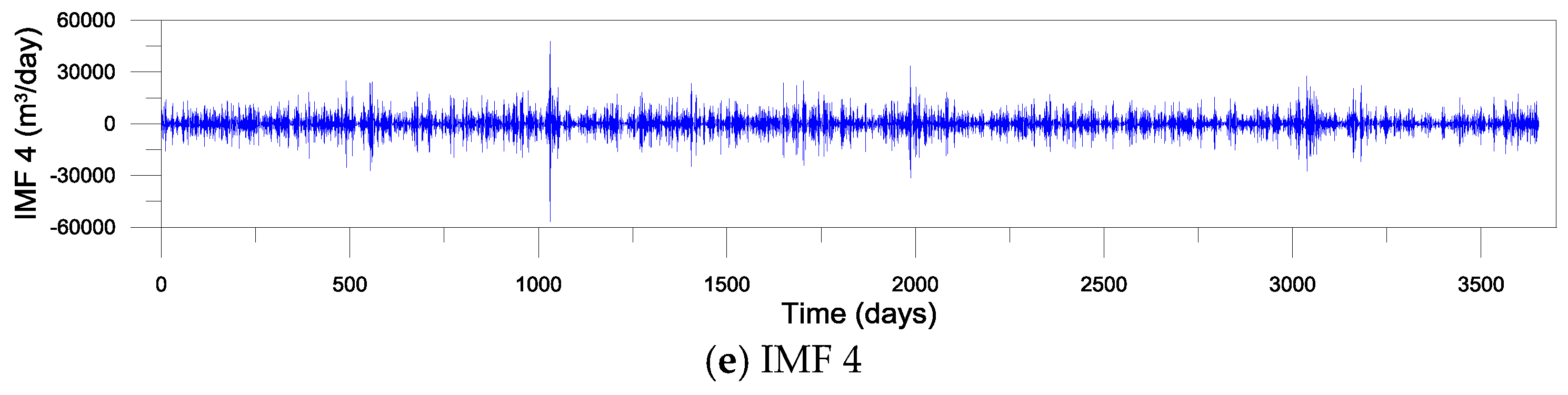
2.2. Variational Mode Decomposition (VMD)

VMD, which is developed by Dragomiretskiy and Zosso [19], is a non-recursive and adaptive time-frequency analysis method. The VMD decomposes an original time series f into K sub-time series called intrinsic mode functions (IMFs). The IMFs can be obtained by updating Equations (1)–(3) until convergence [19].

$${\widehat{u}}_k^{n+1}(\omega )=\frac{\widehat{f}(\omega )-{\displaystyle \sum _{i<k}{\widehat{u}}_i^{n+1}(\omega )-{\displaystyle \sum _{i>k}{\widehat{u}}_i^n(\omega )+{\widehat{\lambda }}^n(\omega )/2}}}{1+2\alpha {(\omega -{\omega }_k^n)}^2}$$

(1)

$${\omega }_k^{n+1}=\frac{{\displaystyle {\int }_0^{\infty }\omega {\left|{\widehat{u}}_k^{n+1}(\omega )\right|}^{2}d\omega }}{{\displaystyle {\int }_0^{\infty }{\left|{\widehat{u}}_k^{n+1}(\omega )\right|}^{2}d\omega }}$$

(2)

$${\widehat{\lambda }}^{n+1}(\omega )={\widehat{\lambda }}^n(\omega )+\tau \left[\widehat{f}(\omega )-{\displaystyle \sum _k{\widehat{u}}_k^{n+1}(\omega )}\right]$$

(3)

where ${\widehat{u}}_k^n$ = the kth mode in nth iteration, $\widehat{f}$ = the Fourier transform of f, ${\omega }_k^n$ = the kth center frequency in nth iteration, ${\widehat{\lambda }}^n$ = the Lagrange multiplier in nth iteration, $\alpha$ = the quadratic penalty factor, $\tau$ = the time step of dual ascent. For the theoretical details of VMD, one can refer to Dragomiretskiy and Zosso [19].

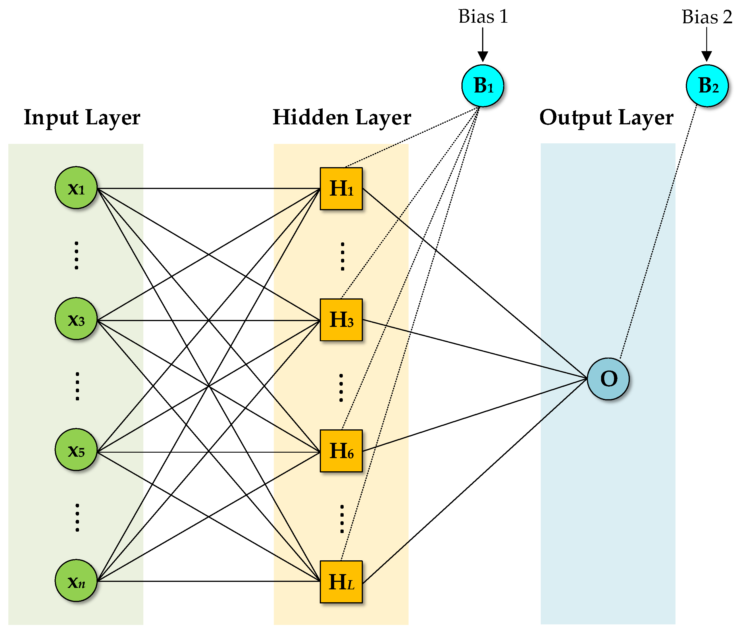
2.3. Artificial Neural Network (ANN)

ANN is an artificial intelligence (AI) model for solving various problems including classification and regression [29]. Multilayer perceptron (MLP) is a kind of feedforward ANN organized into layers with multiple neurons [30], which has been widely applied in hydrological fields. Figure 2 represents the general structure of three-layer MLP. The neurons of the input layer receive the input vectors (lagged water demands), and output values (forecasted water demands) are yielded from the neuron of the output layer. The hidden layer, which is the middle layer of MLP, connects the neurons of the input and output layers. The MLP can be represented as Equation (4) [31]:

$${\widehat{y}}_j={\displaystyle \sum _{i=1}^L{\mathsf{\beta }}_{i}h(w_i\cdot x_j+b_i)+{\mathsf{\beta }}_0,\hspace{1em}j=1,\hspace{0.17em}2,\hspace{0.17em}\cdots ,\hspace{0.17em}N}$$

(4)

where $x_j$ and ${\widehat{y}}_j$ = the input and output vectors, $w_i$ and ${\mathsf{\beta }}_i$ = the weights for the hidden and output layers, $b_i$ and ${\mathsf{\beta }}_0$ = the biases for the hidden and output layers, L = the number of the neurons of hidden layer, N = the length of time series data, and h = the transfer function. The determination of the parameters (weights and biases) of MLP, which is called model learning, is conducted through learning algorithms such as backpropagation (BP). The detailed theoretical background of ANN can be found in Alpaydin [32].

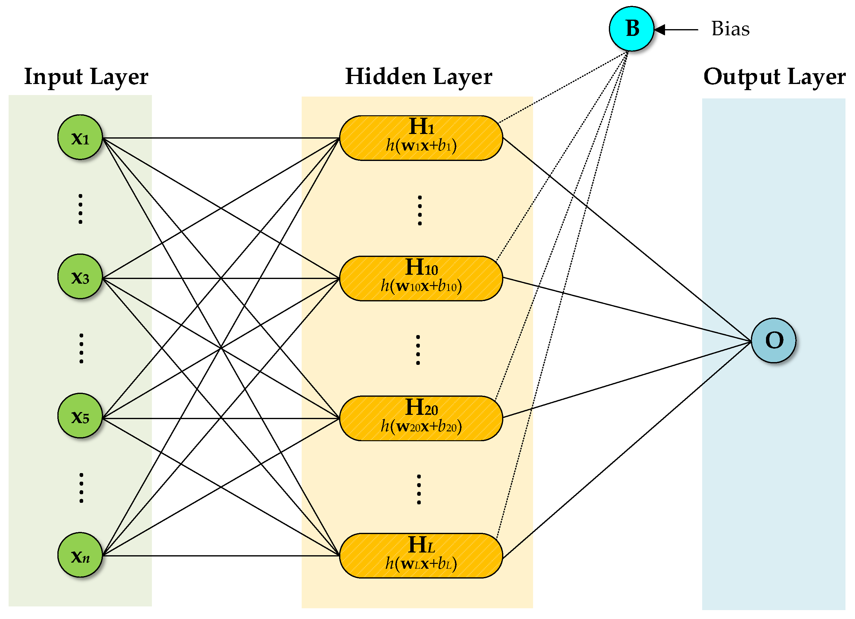
2.4. Extreme Learning Machine (ELM)

ELM is a least square-based single-hidden layer feed-forward neural networks (SLFNs) [33]. In terms of training speed and generalization capability, ELM is known to be superior to conventional ANN [34]. The SLFN with the weights and biases generated randomly can be expressed as Equation (5) and written compactly as Equation (6).

$${\displaystyle \sum _{i=1}^L{\mathsf{\beta }}_{i}h(w_i\cdot x_j+b_i)=t_j,\hspace{0.17em}\hspace{0.17em}\hspace{0.17em}i=1,\hspace{0.17em}2,\hspace{0.17em}\cdots ,\hspace{0.17em}L,\hspace{0.17em}j=1,\hspace{0.17em}2,\hspace{0.17em}\cdots ,\hspace{0.17em}N}$$

(5)

$$H\mathsf{\beta }=T$$

(6)

where $H=h(w_i\cdot x_j+b_i)$ = the matrix comprised of the outputs from hidden neurons, h = the transfer function, $w_i={\left[w_{i1},\hspace{0.17em}{w}_{i2},\hspace{0.17em}\cdots ,\hspace{0.17em}{w}_{in}\right]}^{\mathrm{T}}$ = the ith weight vector between input and hidden neurons, $x_j={[x_{j1},x_{j2},\dots ,x_{jn}]}^{\mathrm{T}}$ = the jth input vectors, $b_i$ = the ith bias for hidden neurons, L and N = the number of hidden neurons and the data length, respectively, $\mathsf{\beta }={\left[{\mathsf{\beta }}_1^{\mathrm{T}},\hspace{0.17em}{\mathsf{\beta }}_2^{\mathrm{T}},\hspace{0.17em}\cdots ,\hspace{0.17em}{\mathsf{\beta }}_L^{\mathrm{T}}\right]}_{L\times m}^{\mathrm{T}}$ = the matrix comprised of weights between hidden and output neurons, ${\mathsf{\beta }}_i={\left[{\mathsf{\beta }}_{i1},\hspace{0.17em}{\mathsf{\beta }}_{i2},\hspace{0.17em}\cdots ,\hspace{0.17em}{\mathsf{\beta }}_{im}\right]}^{\mathrm{T}}$ = the ith weight vectors between hidden and output neurons, and $T={\left[t_1^{\mathrm{T}},\hspace{0.17em}{t}_2^{\mathrm{T}},\hspace{0.17em}\cdots ,\hspace{0.17em}{t}_N^{\mathrm{T}}\right]}_{N\times m}^{\mathrm{T}}$ = the matrix comprised of target vectors $t_j\in {ℝ}^m$.

Unlike conventional ANN, the β is analytically determined by the method of least squares as Equation (7).

$$\widehat{\mathsf{\beta }}=H^{†}T$$

(7)

where $H^{†}=P{H}^{\mathrm{T}}$ is the Moore-Penrose generalized inverse of H, and $P={\left(H^{\mathrm{T}}H\right)}^{-1}$ is the inverse of the covariance matrix of H. Figure 3 represents the general structure of ELM model used in this study. For detailed theoretical background on the ELM, one can refer to Huang et al. [33].

2.5. VMD-Based Water Demand Forecasting

VMD-based machine learning models (VMD-ANN and VMD-ELM) for water demand forecasting are to couple VMD and single machine learning models (ANN and ELM), respectively. VMD was adopted as a time series decomposition method for decomposing water demand time series into IMFs, and ANN and ELM models were used for model learning and forecasting for each IMF. Figure 4 shows the flowchart of VMD-based water demand forecasting consisting of the following four steps:

Step 1.

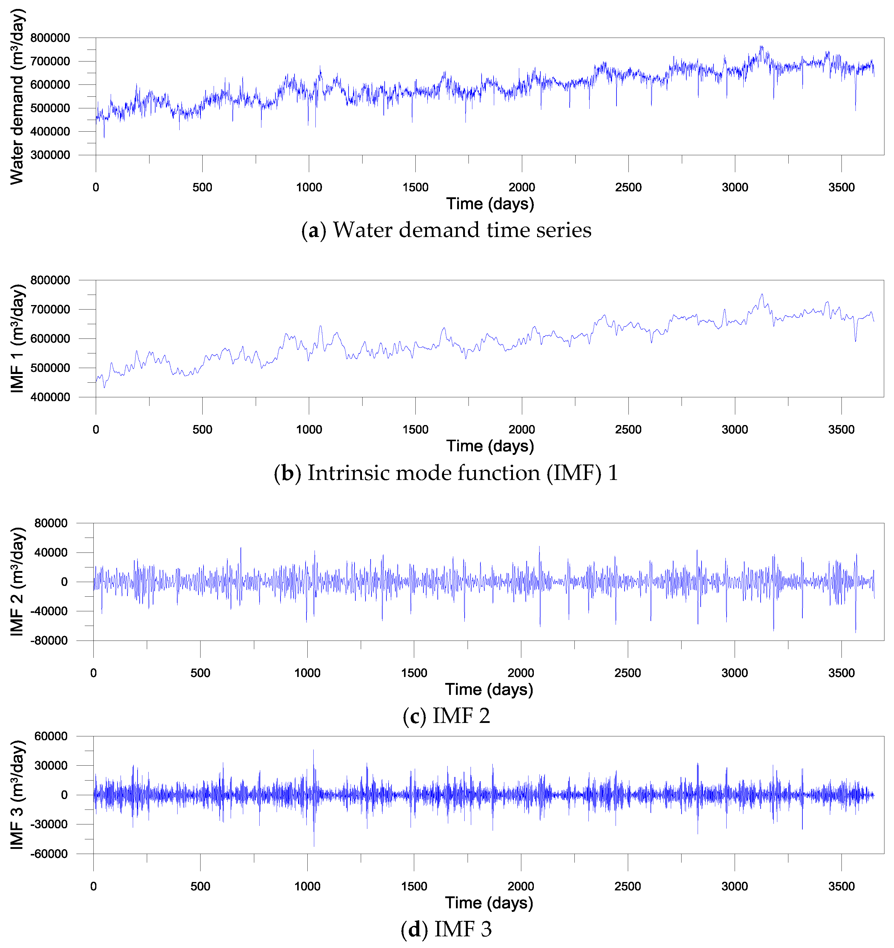
Decomposition: Water demand time series is decomposed into IMFs using VMD.

Step 2.

Model learning: ANN and ELM models are learned for each IMF.

Step 3.

IMF forecasts: ANN and ELM models produce forecasted values for each IMF.

Step 4.

Final forecasts: Summing the forecasted IMFs produces the final water demand forecasts.

2.6. Performance Evaluation Indices

In this study, multiple performance indices were used for evaluating the model performances. Mathematical expressions and ranges for the performance indices are presented in

Table 2. Mathematical expressions and ranges for performance indices.

Performance Indices		Equations	Ranges
Absolute errors	MAE	$MAE=\frac{1}{N}{\displaystyle \sum _{i=1}^N\left|Q_i-{\widehat{Q}}_i\right|}$	$[0,\hspace{0.17em}\infty ]$
	RMSE	$RMSE=\sqrt{\frac{{\displaystyle \sum _{i=1}^N{(Q_i-{\widehat{Q}}_i)}^2}}{N}}$	$[0,\hspace{0.17em}\infty ]$
	R4MS4E	$R4MS4E=\sqrt[4]{\frac{1}{N}{\displaystyle \sum _{i=1}^N{\left(Q_i-{\widehat{Q}}_i\right)}^4}}$	$[0,\hspace{0.17em}\infty ]$
Relative errors	MARE	$MARE=\frac{1}{N}{\displaystyle \sum _{i=1}^N\frac{\left|Q_i-{\widehat{Q}}_i\right|}{Q_i}}$	$[0,\hspace{0.17em}\infty ]$
	MdAPE	$MdAPE=Median\left(\left|\frac{Q_i-{\widehat{Q}}_i}{Q_i}\right|\times 100\right)$	$[0,\hspace{0.17em}\infty ]$
Dimensionless errors	MCE	$MC{E}_j=1-\frac{{\displaystyle \sum _{i=1}^N{\left|Q_i-{\widehat{Q}}_i\right|}^j}}{{\displaystyle \sum _{i=1}^N{\left|Q_i-\overline{Q}\right|}^j}}$ with $j\in \mathbb{\mathbb{N}}$	$[-\infty ,\hspace{0.17em}1]$
	MIOA	$MIO{A}_j=1-\frac{{\displaystyle \sum _{i=1}^N{\left|Q_i-{\widehat{Q}}_i\right|}^j}}{{\displaystyle \sum _{i=1}^N{\left(\left|{\widehat{Q}}_i-\overline{Q}\right|+\left|Q_i-\overline{Q}\right|\right)}^j}}$ with $j\in \mathbb{\mathbb{N}}$	$[0,\hspace{0.17em}1]$

${\widehat{Q}}_i$: forecasted water demand, $Q_i$: observed water demand; $\overline{Q}$: mean of observed water demand; and N: data length.

. Since there is no universal performance index, it is desirable to choose the indices that are appropriate for a particular application. Furthermore, it is common to use multiple performance indices since there are pros and cons in each index [35,36]. The performance indices used in this study are categorized as absolute, relative, and dimensionless errors. The absolute errors include the mean absolute error (MAE), the root mean squared error (RMSE), and the fourth root mean quadrupled error (R4MS4E). RMSE and R4MS4E are sensitive to forecasting errors for peak and high data values, and thus can be good performance indices for high data values. In contrast, MAE is evaluated based on all deviations without being weighted to lower and higher data values. MAE, RMSE, and R4MS4E have the advantage that they can represent the size of a typical error effectively since they are evaluated in the same unit as the original data. For a perfect model, MAE, RMSE, and R4MS4E would be zero [36]. The mean absolute relative error (MARE) and median absolute percentage error (MdAPE) belong to relative errors. MARE is a good index for low data values since it is more affected to forecasting errors for low data values. MdAPE is similar to MARE but it has the advantage that it is less sensitive to skewed error distributions and outliers. For a perfect model, MARE and MdAPE would be zero [36]. The dimensionless errors include the modified versions of the coefficient of efficiency (CE) and the index of agreement (IOA). The CE and IOA have the drawback that they can overestimate the model performance for peak data values. The modified CE (MCE) and modified IOA (MIOA) for j = 1 can reduce the overestimation for peak data values and represent better overall evaluation, whereas larger values of j can be used for the performance evaluation of high data values [35]. For a perfect model, MCE and MIOA would be one [35,36].

3. Results and Discussion

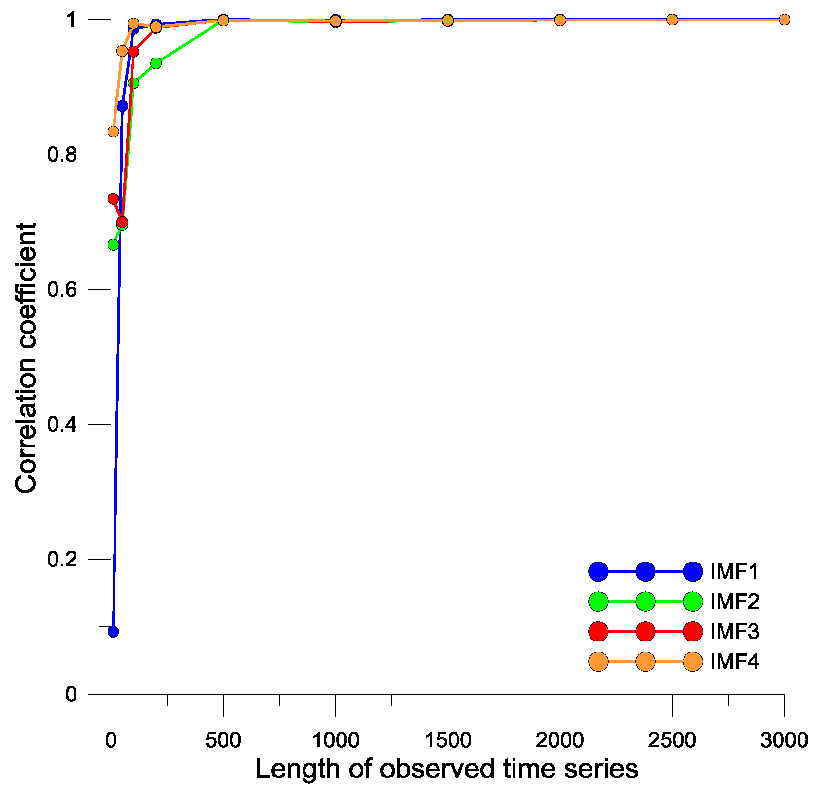
3.1. Development of Single and VMD-Based Forecasting Models

To develop VMD-based water demand models, water demand time series should first be decomposed using the VMD. The decomposition results depend on the quadratic penalty factor (α) and the number of IMFs (K). In this study, the values of α and K were determined based on the following trial-and-error method:

Step 1.

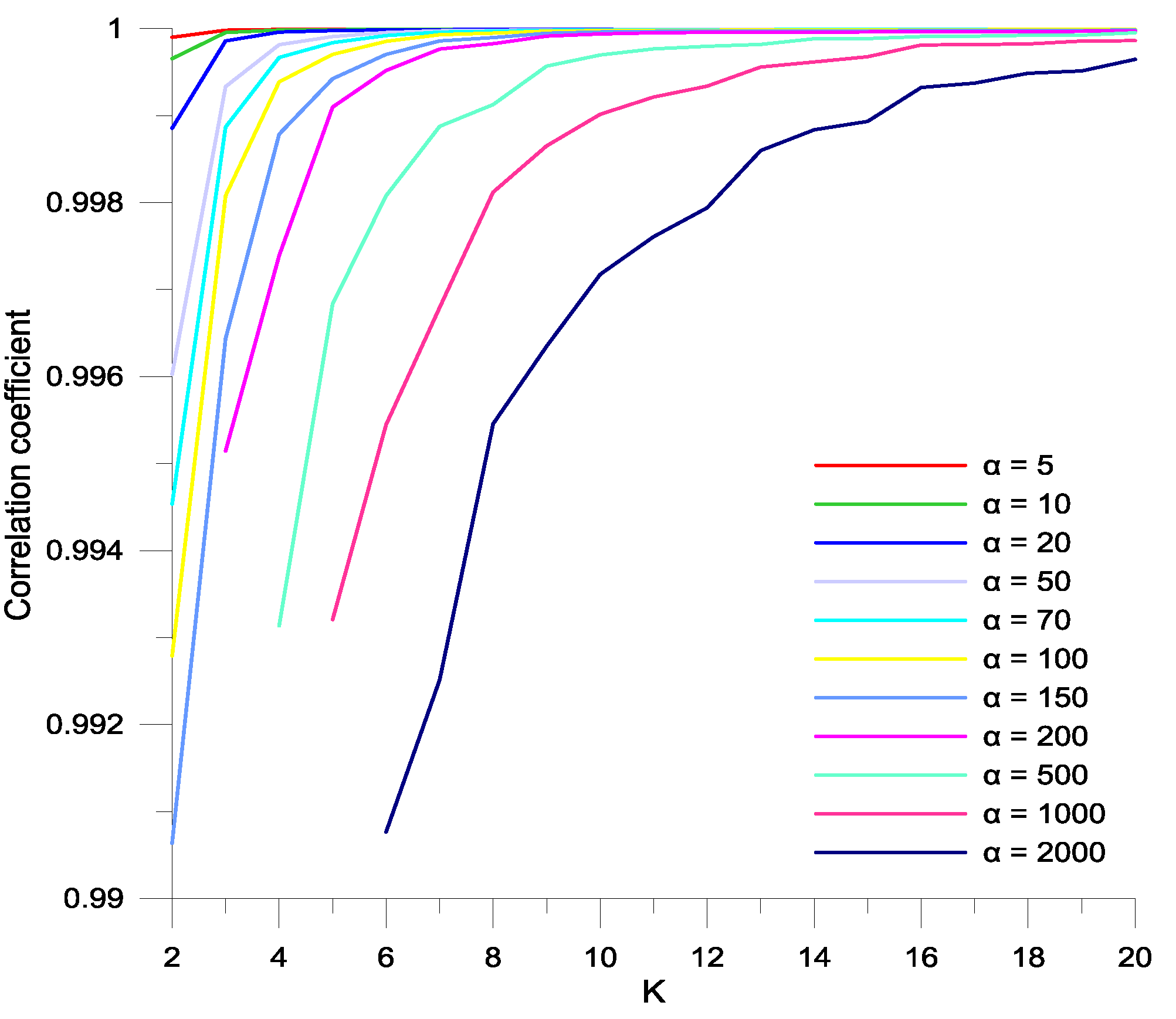
For K = {2, 3, ......, 20} and α = {5, 10, 20, 50, 70, 100, 150, 200, 500, 1000, 2000}, the corresponding IMFs are generated from water demand time series.

Step 2.

For each set of K and α values, the IMFs are summed to reconstruct the water demand time series.

Step 3.

Correlation coefficients (r) between original and reconstructed water demand time series are estimated.

Step 4.

The sets of K and α values corresponding to $r\approx 1$ are selected.

Step 5.

The optimal values of K and α are selected based on the performances of VMD-based forecasting models.

Figure 5 represents the correlation coefficients between the water demand time series and the reconstructed time series for different K and α values. Based on Figure 5, the sets of K and α values corresponding to $r\approx 1$ were selected and then K = 4 and α = 5 producing the best performance of VMD-based forecasting models were selected as the optimal values. Using the K and α values, the original water demand time series was decomposed into four sub-time series (IMF 1-IMF 4) as seen in Figure 6.

For developing forecasting models using ANN and ELM, the potential influencing input variables should be selected in advance. Various lag times for daily water demand time series were considered in this study. The optimal lag time was determined by autocorrelation function (ACF), partial autocorrelation function (PACF), and average mutual information (AMI) [37]. The structure of input and target variables for the ANN and ELM models is as follows:

$$Q_{t+i}=f(Q_{t-5},\hspace{0.17em}{Q}_{t-4},\hspace{0.17em}{Q}_{t-3},\hspace{0.17em}{Q}_{t-2},\hspace{0.17em}{Q}_{t-1},\hspace{0.17em}{Q}_t)$$

(8)

where $Q_{t-j}$ = the input water demand time series lagged by j days (j = 0, 1, ......, 5), $Q_{t+i}$ = the target water demand time series for lead time i day (i = 1, 2, ......, 7), and f = the ANN and ELM models. In the same manner, the structure of input and target variables for VMD-ANN and VMD-ELM models is determined as follows:

$$IMF{1}_{t+i}=f(IMF{1}_{t-9},\hspace{0.17em}IMF{1}_{t-8},\hspace{0.17em}\dots ,\hspace{0.17em}IMF{1}_{t-1},\hspace{0.17em}IMF{1}_t)$$

(9)

$$IMF{2}_{t+i}=f(IMF{2}_{t-1},\hspace{0.17em}IMF{2}_t)$$

(10)

$$IMF{3}_{t+i}=f(IMF{3}_{t-1},\hspace{0.17em}IMF{3}_t)$$

(11)

$$IMF{2}_{t+i}=f(IMF{2}_{t-1},\hspace{0.17em}IMF{2}_t)$$

(12)

Figure 7 shows correlation coefficients between IMFs obtained from the entire water demand time series and ones from the partial water demand time series with different lengths. From Figure 7, it was seen that time series decomposition by VMD was dependent on the length of water demand time series. When the length of the partial time series was more than 500, the decomposition result was almost the same as the result for the entire time series. Thus, for real-time forecasting, VMD should be executed whenever new observations are acquired, and at least 500 previous time series data should be used for time series decomposition.

In ANN and ELM modeling, selecting the optimal number of hidden neurons is a critical step since it affects the model performance. A trial-and-error approach [37] was utilized for determining the optimal number in this study. In most hydrological fields, the logistic sigmoid function has been widely applied to ANN modeling in order to compute the output of each neuron [26]. The function is also applied to ANN and ELM modeling in this study. Furthermore, the ANN model was learned by BP algorithm and the default values of learning parameters (learning and momentum rates) presented by Zell et al. [38] were used. When considering both processing speed and accuracy, it is more efficient to use the appropriate small values of learning parameters than to determine them using a trial-and-error approach [39]. More information on this can be found in Rumelhart et al. [40], Pao [41], and Seo et al. [18].

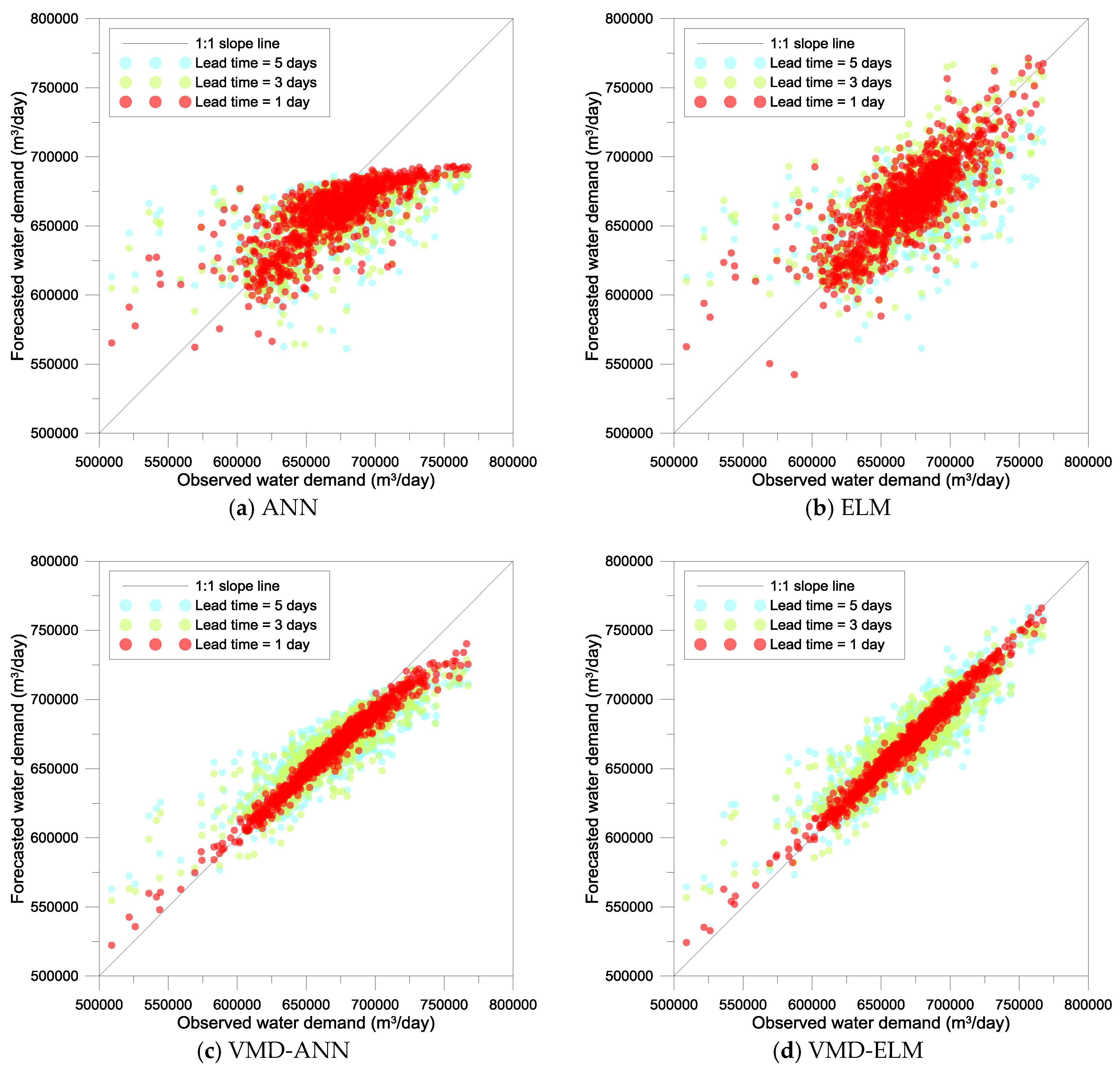
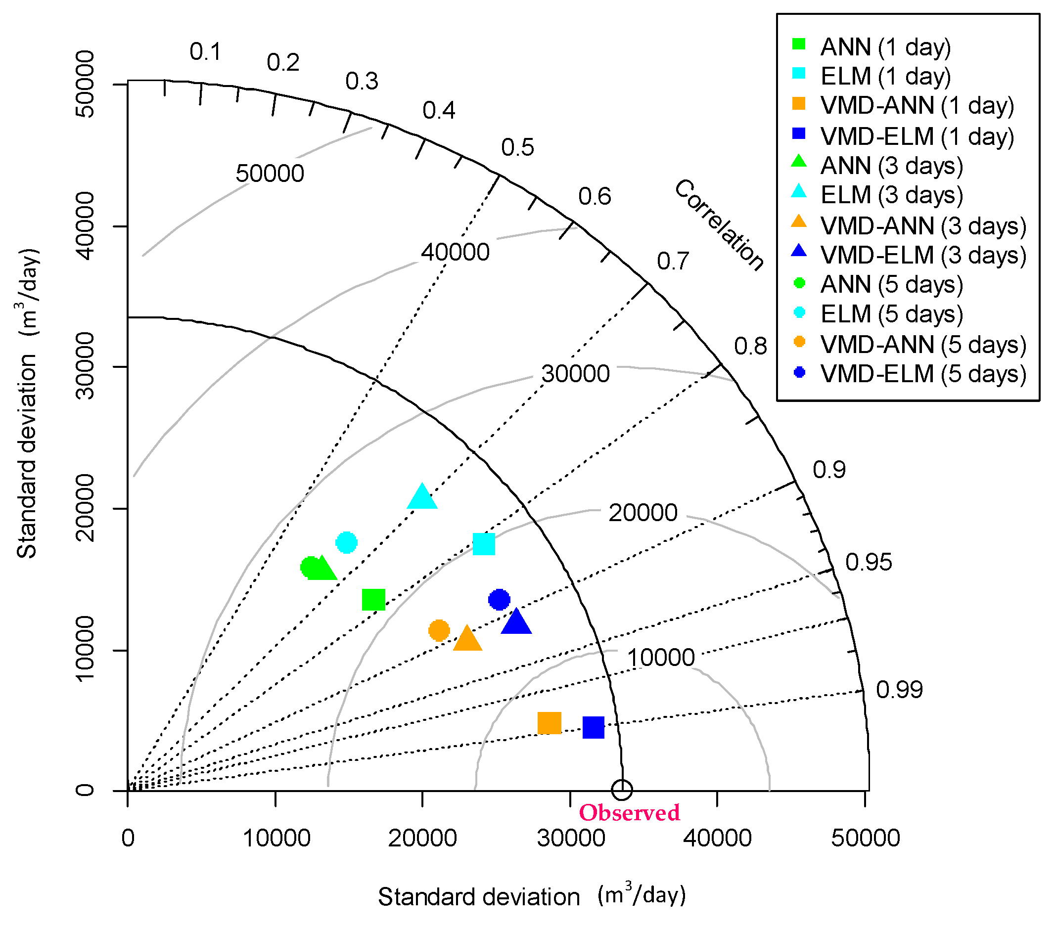
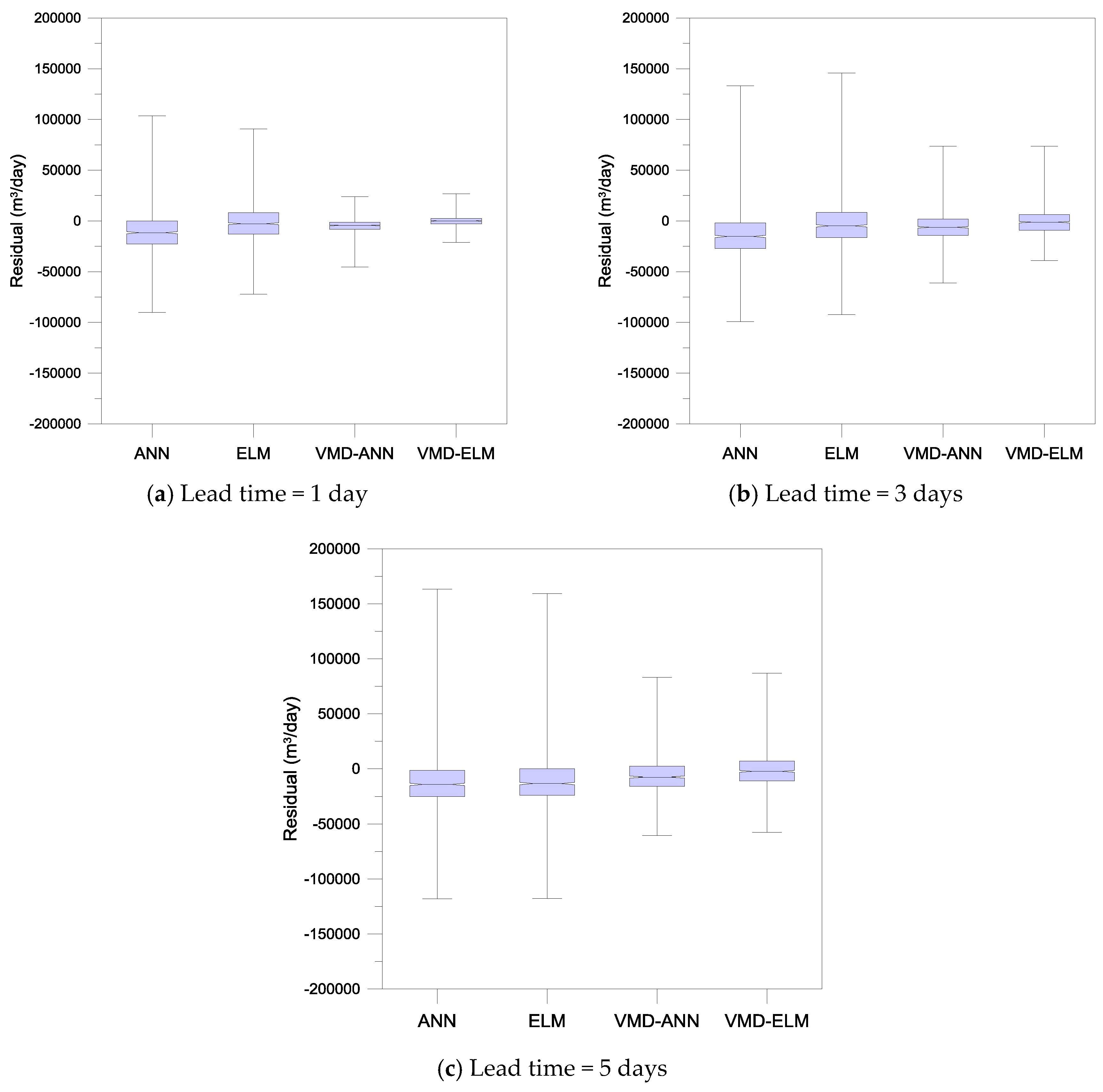
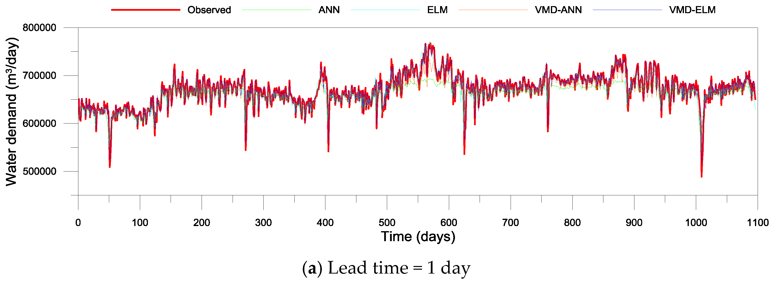
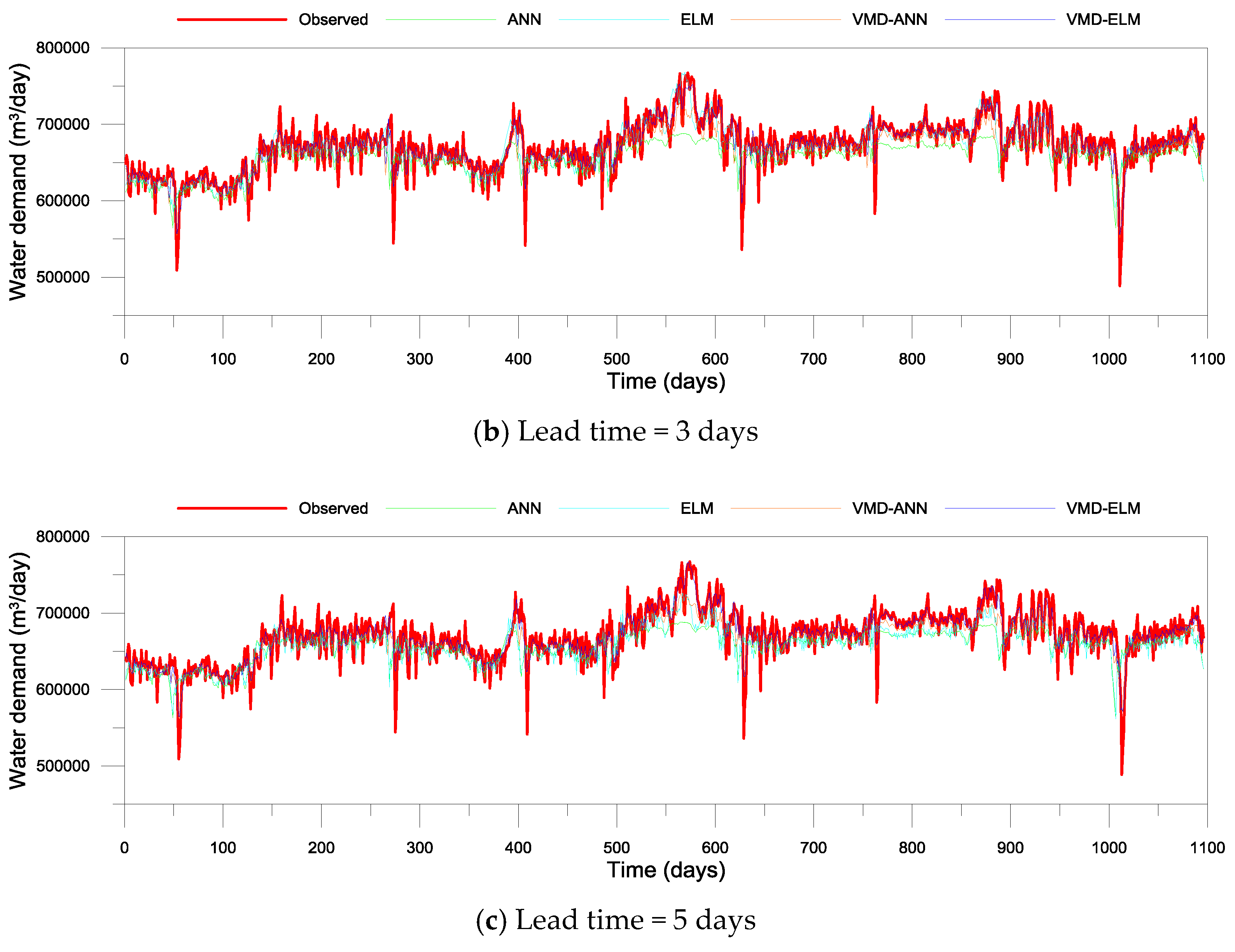
3.2. Performance Evaluation

In this study, absolute error indices (MAE, RMSE, and R4MS4E), relative error indices (MARE and MdAPE), and dimensionless error indices (MCE and MIOA) were employed in order to evaluate and compare model performances for testing data. MCE and MIOA with j = 1 (MCE₁ and MIOA₁) were used to evaluate overall performances, and MCE and MIOA with j = 2 and 3 (MCE₂, MCE₃, MIOA₂, and MIOA₃) were employed to evaluate performances for high water demands. The results of performance evaluation for testing data are summarized in

Table 3. Performance evaluation for testing data.

Models	Lead Times (Days)	MAE (m3/day)	RMSE (m3/day)	R4MS4E (m3/day)	MARE	MdAPE	MCE1	MIOA1	MCE2	MIOA2	MCE3	MIOA3
ANN	1	18,694	24,366	34,700	0.028	2.330	−0.141	0.576	−0.284	0.797	−0.422	0.901
	2	21,322	27,658	39,636	0.032	2.592	−0.362	0.516	−0.831	0.728	−1.533	0.835
	3	22,714	29,468	42,812	0.035	2.851	−0.460	0.491	−1.086	0.692	−2.088	0.792
	4	21,924	29,203	43,984	0.033	2.616	−0.431	0.498	−1.106	0.688	−2.296	0.775
	5	22,044	29,447	45,190	0.034	2.606	−0.432	0.496	−1.126	0.683	−2.421	0.761
	6	23,444	30,669	45,419	0.036	2.824	−0.514	0.478	−1.282	0.666	−2.610	0.752
	7	25,252	32,166	45,993	0.039	3.245	−0.639	0.452	−1.551	0.644	−3.065	0.739
ELM	1	14,620	19,928	30,446	0.022	1.622	0.421	0.693	0.648	0.894	0.783	0.961
	2	16,703	23,184	37,696	0.025	1.849	0.338	0.643	0.523	0.846	0.625	0.920
	3	17,890	24,932	40,900	0.027	2.003	0.291	0.618	0.449	0.822	0.527	0.898
	4	19,809	26,841	42,127	0.030	2.285	0.216	0.558	0.361	0.767	0.452	0.857
	5	21,006	28,235	43,937	0.031	2.510	0.169	0.533	0.294	0.740	0.372	0.832
	6	19,585	27,322	43,623	0.029	2.161	0.226	0.594	0.339	0.793	0.398	0.875
	7	20,375	27,516	43,073	0.031	2.416	0.195	0.561	0.330	0.770	0.412	0.858
VMD-ANN	1	6417	8719	13,455	0.009	0.717	0.746	0.864	0.933	0.981	0.982	0.997
	2	8852	11,899	17,349	0.013	1.004	0.649	0.808	0.874	0.961	0.957	0.993
	3	12,166	16,154	23,847	0.018	1.432	0.518	0.728	0.769	0.923	0.891	0.978
	4	14,291	18,210	25,581	0.021	1.824	0.434	0.682	0.706	0.902	0.857	0.972
	5	13,701	18,046	26,735	0.020	1.655	0.458	0.686	0.711	0.899	0.849	0.967
	6	16,225	21,094	30,659	0.024	1.987	0.359	0.631	0.606	0.860	0.765	0.946
	7	17,058	23,013	35,325	0.026	1.945	0.326	0.609	0.531	0.827	0.664	0.916
VMD-ELM	1	3637	4927	7519	0.005	0.403	0.856	0.927	0.978	0.994	0.997	0.999
	2	6327	8643	12,999	0.010	0.696	0.749	0.868	0.934	0.981	0.983	0.997
	3	10,156	13,824	21,805	0.015	1.161	0.598	0.784	0.830	0.949	0.925	0.987
	4	10,068	13,691	21,945	0.015	1.159	0.601	0.784	0.834	0.949	0.926	0.987
	5	11,888	16,010	25,408	0.018	1.393	0.530	0.745	0.773	0.930	0.884	0.979
	6	12,836	17,513	27,604	0.019	1.460	0.493	0.728	0.728	0.917	0.847	0.972
	7	14,405	20,077	31,553	0.022	1.634	0.431	0.696	0.643	0.890	0.766	0.956

.

For single forecasting models (ANN and ELM), the ELM model yielded lower MAE and higher MCE₁ and MIOA₁ than ANN model. ANN model produced negative MCE₁. These indicated that ELM model represented better overall performance compared with ANN model, and ANN model performed worse than a “no knowledge” model. ELM model yielded lower values of MARE and MdAPE compared with ANN model. ELM model produced better performance than ANN model for low water demands. Furthermore, the ELM model yielded lower values of RMSE and R4MS4E and higher values of MCE₂, MIOA₂, MCE₃, and MIOA₃ than ANN model. ANN model produced negative values of MCE₂ and MCE₃. These indicated that ELM model represented better performance for higher water demands compared with ANN model, and ANN model produced worse performance than a “no knowledge” model. Consequently, it was found from the results of single forecasting models that ELM model performed better over the entire range of testing data compared with ANN model.

For VMD-based forecasting models (VMD-ANN and VMD-ELM), VMD-ELM model yielded better performance indices than VMD-ANN model. For example, the MAE values of VMD-ELM model were lower than those of VMD-ANN model, and the MCE₁ and MIOA₁ values of VMD-ELM model were higher than those of VMD-ANN model. These represented that the overall performance of VMD-ELM model was better compared with VMD-ANN model. Furthermore, the values of MARE and MdAPE for VMD-ELM model were smaller than those for VMD-ANN model, and VMD-ELM produced lower values of RMSE and R4MS4E and higher values of MCE₂, MIOA₂, MCE₃, and MIOA₃ compared with VMD-ANN models. These results represented that VMD-ELM model performed better than VMD-ANN model for low and high water demands. Consequently, from the results of VMD-based forecasting models, it was found that VMD-ELM model outperformed VMD-ANN model over the entire range of testing data.

These results are due to the theoretical characteristics of ANN and ELM models. For the ANN model, gradient descent-based learning algorithms such as BP algorithm adjust all the parameters iteratively and require many iterative steps for obtaining satisfactory performance. Thus, the learning process is very slow, and it is difficult for the ANN model to reach the minimum training error due to infinite training iteration and local minima. In addition, the ANN model may be over-trained by gradient descent-based learning and produce worse generalization performance. Gradient descent-based learning algorithms only ty to reach the smallest training error, and do not consider the magnitude of the weights. These characteristics make it difficult for the ANN model to achieve the best generalization performance [25]. On the other hand, the ELM model is considered as a linear system after the input weights and the biases of the hidden layer are assigned randomly. Namely, the input weights and the biases of the hidden layer do not need to be tuned and any iterative learning process is also not required. The output weights of the ELM model can be determined analytically by finding the smallest norm least-squares solution for the linear system using the Moore-Penrose generalized inverse. Thus, the ELM model can produce the minimum training error, the smallest norm of weights, and the best generalization performance [25].

From the comparison of single and VMD-based forecasting models, VMD-ANN and VMD-ELM models represented better performance compared with ANN and ELM models. For instance, VMD-ANN and VMD-ELM models yielded lower MAE and higher MCE₁ and MIOA₁ values than ANN and ELM models, which represented better overall performance for VMD-ANN and VMD-ELM models. Furthermore, VMD-ANN and VMD-ELM models yielded lower MARE and MdAPE values than ANN and ELM models. For VMD-ANN and VMD-ELM models, the values of RMSE and R4MS4E were lower and the values of MCE₂, MIOA₂, MCE₃, and MIOA₃ were higher compared with ANN and ELM models. These results represented that VMD-ANN and VMD-ELM models produced better performance than ANN and ELM models for low and high water demands. Therefore, from the comparison of single and VMD-based forecasting models, it was found that VMD-ANN and VMD-ELM models outperformed ANN and ELM models over the entire range of testing data, VMD-ELM model produced the best performance, and the performances of ANN and ELM models were able to be improved by VMD.

In general, water demand time series is a combination of different time-frequency features and has strong nonlinearity and non-stationarity. In this study, VMD decomposes an original water demand time series into multiple modes (low- and high-frequency modes), and then the modes are updated by Wiener filtering [42]. Since the modes represent simpler patterns than the original time series, the ANN and ELM models can be learned more effectively using the modes as training datasets than using the original time series. Especially, since low-frequency mode (IMF 1), which represents the trend component of water demand time series, can be modeled very accurately by the single forecasting models, the performance of water demand forecasting can be improved significantly by VMD. Thus, for water demand time series with strong nonlinearity and non-stationarity, VMD-based forecasting models can produce better performance than single forecasting models.

Figure 8 shows scatter diagrams for forecasted and observed water demands. It was observed from Figure 8 that the scatter points of VMD-ANN and VMD-ELM models were closer to 1:1 slope line than those of ANN and ELM models. Based on scatter diagrams, VMD-ELM model produced the most accurate result among all other models. Although VMD-ANN and VMD-ELM models represented similar dispersion around 1:1 slope line, VMD-ANN model yielded underestimated values for high water demands. ELM model represented better accuracy than ANN model. Especially, the ANN model produced greatly underestimated result for high water demands. Although VMD was able to improve the underestimation of ANN model for high water demands, the underestimation was not resolved completely even in VMD-ANN model. Consequently, VMD-ELM model represented better accuracy compared with all other models, in terms of under- and overestimation and dispersion around 1:1 slope line. It was also found from these results that the accuracy of ANN and ELM models was able to be improved significantly by VMD.

Figure 9 shows Taylor diagram for single and VMD-based forecasting models. The diagram provides a graphical summary for the agreement of observed and forecasted patterns, based on correlation coefficient (CC), standard deviation (SD), and centered root-mean-square difference (CRMSD) [43]. In Figure 9, the gray contour lines and black arc represent the values of CRMSD and SD for observed pattern, respectively. The closer a model is to the black hollow circle marker, the closer the forecasted pattern is to the observed pattern. From Figure 9, it was observed that VMD-ANN and VMD-ELM models yielded higher CC and lower CRMSD than ANN and ELM models, and ELM and VMD-ELM models produced SD values closer to the observed pattern compared with ANN and VMD-ANN models. Especially, it was shown that VMD-ELM models were located the closest to the black hollow circle marker among all other models. Consequently, based on Taylor diagram, it can be said that VMD-ANN and VMD-ELM models outperformed ANN and ELM models, and VMD was able to improve the accuracy of ANN and ELM models.

Figure 10 and Figure 11 show residual boxplots and time series plots for single and VMD-based forecasting models, respectively. It was observed from Figure 10 that the ranges (maximum—minimum) and interquartile ranges (third quartile—first quartile) of residuals for VMD-ANN and VMD-ELM models were smaller than those for the ANN and ELM models, and the median values of residuals for the ANN and ELM models were biased in the negative direction from zero compared with VMD-ANN and VMD-ELM models, respectively. Furthermore, it was observed from Figure 11 that VMD-ANN and VMD-ELM models forecasted the observed pattern more accurately than ANN and ELM models. Especially, compared with VMD-ANN and VMD-ELM models, the ANN and ELM models showed greater over- and underestimation for low and high water demands, respectively. These results indicated that VMD was able to reduce the residuals of ANN and ELM models significantly, improve under- and overestimation represented in ANN and ELM models, and thus enhance the accuracy of ANN and ELM models.

From the results obtained from this study, VMD-based forecasting models produced better performances than single forecasting models in daily water demand forecasting. Similar results have also been reported from previous studies dealing with DWT-based hybrid modeling for water demand [7,8,9] and VMD-based hybrid modeling for river stage [17] and rainfall-runoff [18]. VMD decomposes water demand time series, which is a mixture of complex and irregular components, into multiple sub-time series (IMFs). Machine learning-based forecasting models are then constructed for each sub-time series. Since the sub-time series represent simpler temporal patterns than the original time series, the machine learning models can be trained more effectively, and thus water demand time series with strong nonlinearity and non-stationarity can be forecasted more accurately. Furthermore, by applying Wiener filtering, VMD can be more robust to noise affecting the decomposition accuracy of water demand time series negatively and yield narrow-based modes. Due to these characteristics, the VMD not only alleviates the mode mixing but also provides accurate time-frequency features. In addition, since VMD is a non-recursive signal decomposition algorithm, error propagation which inevitably occurs in iterative algorithms does not occur. These characteristics enable the VMD to produce more accurate time-frequency features compared with other signal decomposition methods such as EMD [42,44].

Meanwhile, VMD-based water demand forecasting models can be a more reliable forecasting tool by combining with resampling techniques including simple bootstrap, block bootstrap, Gaussian process regression bootstrap, Bayesian bootstrap, and maximum entropy bootstrap. Hybrid modeling similar to this concept was carried out successfully by Tiwari and Adamowski [7]. They developed a hybrid model (WBNN) coupling simple bootstrap, DWT, and ANN in order to forecast short-term urban water demand and concluded that WBNN model was able to decrease the forecasting uncertainty and thus provide more accurate and reliable water demand forecasts. Therefore, the combined model of resampling techniques, VMD, and machine learning models can be suggested as a future study for improving short-term water demand forecasting.

4. Conclusions

This study investigates the performances of VMD-based water demand forecasting models. VMD and two machine learning models, the ANN and ELM, were employed for the decomposition of water demand time series and the forecasting of sub-time series, respectively. The performances of single forecasting models (ANN and ELM) and VMD-based forecasting models (VMD-ANN and VMD-ELM) are evaluated based on performance indices and graphical analysis. For single forecasting models, the ELM model outperforms the ANN model. VMD-ANN and VMD-ELM models perform better compared with ANN and ELM models, and the VMD-ELM model achieves the best performance among all the models. From the results of this study, it is revealed that VMD can reduce forecasting error and improve model performance in machine learning-based water demand forecasting. Therefore, VMD-based machine learning models can be effective forecasting tools for short-term water demand with strong nonlinearity and non-stationarity and contribute to operate urban water supply facilities efficiently. This study is limited to short-term water demand forecasting for a specific area. Further studies need to be performed with regard to water demand forecasting for other areas which have demographic, economic, and weather conditions similar to the area where forecasting models are developed.

References

1. House-Peters, L.A.; Chang, H. Urban water demand modeling: Review of concepts, methods, and organizing principles. Water Resour. Res. 2011, 47, W05401. [Google Scholar] [CrossRef]
2. Schuetze, T.; Santiago-Fandiño, V. Quantitative assessment of water use efficiency in urban and domestic buildings. Water 2013, 5, 1172–1193. [Google Scholar] [CrossRef]
3. Hao, L.; Sun, G.; Liu, Y.; Qian, H. Integrated modeling of water supply and demand under management options and climate change scenarios in Chifeng city, China. J. Am. Water Resour. Assoc. 2015, 51, 655–671. [Google Scholar] [CrossRef]
4. Arsiso, B.K.; Tsidu, G.M.; Stoffberg, G.H.; Tadesse, T. Climate change and population growth impacts on surface water supply and demand of Addis Ababa, Ethiopia. Clim. Risk Manag. 2017, 18, 21–33. [Google Scholar] [CrossRef]
5. Lee, J.S.; Kim, J.W. Assessing strategies for urban climate change adaptation: The case of six metropolitan cities in South Korea. Sustainability 2018, 10, 2065. [Google Scholar] [CrossRef]
6. Donkor, E.A.; Mazzuchi, T.A.; Soyer, R.; Roberson, J.A. Urban water demand forecasting: Review of methods and models. J. Water Res. Plan. Manag. 2014, 140, 146–159. [Google Scholar] [CrossRef]
7. Tiwari, M.K.; Adamowski, J. Urban water demand forecasting and uncertainty assessment using ensemble wavelet-bootstrap-neural network models. Water Resour. Res. 2013, 49, 6486–6507. [Google Scholar] [CrossRef] [Green Version]
8. Adamowski, J.; Chan, H.F.; Prasher, S.O.; Ozga-Zielinski, B.; Sliusarieva, A. Comparison of multiple linear and nonlinear regression, autoregressive integrated moving average, artificial neural network, and wavelet artificial neural network methods for urban water demand forecasting in Montreal, Canada. Water Resour. Res. 2012, 48, W01528. [Google Scholar] [CrossRef]
9. Bai, Y.; Wang, P.; Li, C.; Xie, J.; Wang, Y. A multi-scale relevance vector regression approach for daily urban water demand forecasting. J. Hydrol. 2014, 517, 236–245. [Google Scholar] [CrossRef]
10. Brentan, B.M.; Luvizotto, E., Jr.; Herrera, M.; Izquierdo, J.; Pérez-García, R. Hybrid regression model for near real-time urban water demand forecasting. J. Comput. Appl. Math. 2017, 309, 532–541. [Google Scholar] [CrossRef]
11. Arandia, E.; Ba, A.; Eck, B.; McKenna, S. Tailoring seasonal time series models to forecast shot-term water demand. J. Water Res. Plan. Manag. 2016, 142, 1–10. [Google Scholar] [CrossRef]
12. Gagliardi, F.; Alvisi, S.; Kapelan, Z.; Franchini, M. A probabilistic short-term water demand forecasting model based on the Markov chain. Water 2017, 9, 507. [Google Scholar] [CrossRef]
13. Pacchin, E.; Alvisi, S.; Franchini, M. A short-term water demand forecasting model using a moving window on previously observed data. Water 2017, 9, 172. [Google Scholar] [CrossRef]
14. Alvisi, S.; Franchini, M. Assessment of predictive uncertainty within the framework of water demand forecasting using the Model Conditional Processor (MCP). Urban Water J. 2017, 14, 1–10. [Google Scholar] [CrossRef]
15. Anele, A.O.; Hamam, Y.; Abu-Mahfouz, A.M.; Todini, E. Overview, comparative assessment and recommendations of forecasting models for short-term water demand prediction. Water 2017, 9, 887. [Google Scholar] [CrossRef]
16. Anele, A.O.; Todini, E.; Hamam, Y.; Abu-Mahfouz, A.M. Predictive uncertainty estimation in water demand forecasting using the model conditional processor. Water 2018, 10, 475. [Google Scholar] [CrossRef]
17. Seo, Y.; Kim, S.; Singh, V.P. Comparison of different heuristic and decomposition techniques for river stage modeling. Environ. Monit. Assess. 2018, 190, 392. [Google Scholar] [CrossRef] [PubMed]
18. Seo, Y.; Kim, S.; Singh, V.P. Machine learning models coupled with variational mode decomposition: A new approach for modeling daily rainfall-runoff. Atmosphere 2018, 9, 251. [Google Scholar] [CrossRef]
19. Dragomiretskiy, K.; Zosso, D. Variational mode decomposition. IEEE Trans. Signal Process. 2014, 62, 531–544. [Google Scholar] [CrossRef]
20. Polyak, N.; Pearlman, W.A. Stationarity of the Gabor basis and derivation of Janssen’s formula. In Proceedings of the IEEE-SP International Symposium on Time-Frequency and Time-Scale Analysis, Victoria, BC, Canada, 4–6 October 1992. [Google Scholar] [CrossRef]
21. Deo, R.C.; Şahin, M. An extreme learning machine model for the simulation of monthly mean streamflow water level in eastern Queensland. Environ. Monit. Assess. 2016, 188, 90. [Google Scholar] [CrossRef] [PubMed]
22. Yaseen, Z.M.; Jaafar, O.; Deo, R.C.; Kisi, O.; Adamowski, J.; Quilty, J.; El-Shafie, A. Stream-flow forecasting using extreme learning machines: A case study in a semi-arid region in Iraq. J. Hydrol. 2016, 542, 603–614. [Google Scholar] [CrossRef]
23. Bengio, Y.; Simard, P.; Frasconi, P. Learning ling-term dependencies with gradient descent is difficult. IEEE Trans. Neural Netw. 1994, 5, 157–166. [Google Scholar] [CrossRef] [PubMed]
24. Brink, H.; Richards, J.W.; Fetherolf, M. Real-World Machine Learning; Manning Publications Co.: Shelter Island, NY, USA, 2017; ISBN 978-1617291920. [Google Scholar]
25. Huang, G.B.; Zhu, Q.Y.; Siew, C.K. Extreme learning machine: A new learning scheme of feedforward neural networks. In Proceedings of the 2004 IEEE International Joint Conference on Neural Networks, Budapest, Hungary, 25–29 July 2004. [Google Scholar] [CrossRef]
26. Dawson, C.W.; Wilby, R.L. Hydrological modelling using artificial neural networks. Prog. Phys. Geogr. 2001, 25, 80–108. [Google Scholar] [CrossRef]
27. Partal, T.; Cigizoglu, H.K. Estimation and forecasting of daily suspended sediment data using wavelet-neural networks. J. Hydrol. 2008, 358, 317–331. [Google Scholar] [CrossRef]
28. Mohanta, A.; Patra, K.C.; Sahoo, B.B. Anticipate Manning’s coefficient in meandering compound channels. Hydrology 2018, 5, 47. [Google Scholar] [CrossRef]
29. ASCE Task Committee. Artificial neural networks in hydrology. I: Preliminary concepts. J. Hydrol. Eng. 2000, 5, 115–123. [Google Scholar] [CrossRef]
30. Zahmatkesh, Z.; Goharian, E. Comparing machine learning and decision making approaches to forecast long lead monthly rainfall: The city of Vancouver, Canada. Hydrology 2018, 5, 10. [Google Scholar] [CrossRef]
31. Lima, A.R.; Cannon, A.J.; Hsieh, W.W. Forecasting daily streamflow using online sequential extreme learning machines. J. Hydrol. 2016, 537, 431–443. [Google Scholar] [CrossRef]
32. Alpaydin, E. Introduction to Machine Learning, 2nd ed.; The MIT Press: Cambridge, MA, USA, 2010; ISBN 978-0262028189. [Google Scholar]
33. Huang, G.B.; Zhu, Q.Y.; Siew, C.K. Extreme learning machine: Theory and application. Neurocomputing 2006, 70, 489–501. [Google Scholar] [CrossRef]
34. Yu, L.; Dai, W.; Tang, L. A novel decomposition ensemble model with extended extreme learning machine for crude oil price forecasting. Eng. Appl. Artif. Intell. 2016, 47, 110–121. [Google Scholar] [CrossRef]
35. Krause, P.; Boyle, D.P.; Bäse, F. Comparison of different efficiency criteria for hydrological model assessment. Adv. Geosci. 2005, 5, 89–97. [Google Scholar] [CrossRef]
36. Dawson, C.W.; Abrahart, R.J.; See, L.M. HydroTest: A web-based toolbox of evaluation metrics for the standardized assessment of hydrological forecasts. Environ. Model. Softw. 2007, 22, 1034–1052. [Google Scholar] [CrossRef]
37. Seo, Y.; Kim, S.; Kisi, O.; Singh, V.P. Daily water level forecasting using wavelet decomposition and artificial neural intelligence techniques. J. Hydrol. 2015, 520, 224–243. [Google Scholar] [CrossRef]
38. Zell, A.; Mamier, G.; Mache, M.V.N.; Hübner, R.; Dörin, S.; Hermann, K.U. SNNS Stuttgart Neural Network Simulator v. 4.2, User Manual. University of Stuttgart/University of Tübingen. 1998. Available online: http://www.ra.cs.uni-tuebingen.de/downloads/SNNS/SNNSv4.2.Manual.pdf (accessed on 30 June 2018).
39. Dai, H.; MacBeth, C. Effects of learning parameters on learning procedure and performance of a BPNN. Neural Netw. 1997, 10, 1505–1521. [Google Scholar] [CrossRef]
40. Rumelhart, D.; Hinton, G.E.; Williams, R.J. Learning representations by back-propagating errors. Nature 1986, 323, 533–536. [Google Scholar] [CrossRef]
41. Pao, Y.H. Adaptive Pattern Recognition and Neural Networks; Addison-Wesley Publishing Company, Inc.: New York, NY, USA, 1988; ISBN 978-0201125849. [Google Scholar]
42. Shi, P.; Yang, W. Precise feature extraction from wind turbine condition monitoring signals by using optimised variational mode decomposition. IET Renew. Power Gener. 2017, 11, 245–252. [Google Scholar] [CrossRef]
43. Taylor, K.E. Summarizing multiple aspects of model performance in a single diagram. J. Geophys. Res. Atmos. 2001, 106, 7183–7192. [Google Scholar] [CrossRef] [Green Version]
44. Sun, G.; Chen, T.; Wei, Z.; Sun, Y.; Zang, H.; Chen, S. A carbon price forecasting model based on variational mode decomposition and spiking neural networks. Energies 2016, 9, 54. [Google Scholar] [CrossRef]
Figure 1. Water supply areas and location of water purification plant.
Hydrology 05 00054 g001
Figure 2. General structure of multilayer perceptron (MLP)-type artificial neural network (ANN).
Hydrology 05 00054 g002
Figure 3. General structure of extreme learning machine (ELM).
Hydrology 05 00054 g003
Figure 4. Flowchart for variational mode decomposition (VMD)-based water demand forecasting.
Hydrology 05 00054 g004
Figure 5. Correlation relationship between original water demand time series and reconstructed time series for different K and α values.
Hydrology 05 00054 g005
Figure 6. Water demand time series and IMFs.
Hydrology 05 00054 g006aHydrology 05 00054 g006b
Figure 7. Correlation coefficients between IMFs obtained from the entire water demand time series and ones from the partial water demand time series with different lengths.
Hydrology 05 00054 g007
Figure 8. Scatter diagrams for single and VMD-based forecasting models.
Hydrology 05 00054 g008
Figure 9. Taylor diagram for single and VMD-based forecasting models.
Hydrology 05 00054 g009
Figure 10. Residual boxplots for single and VMD-based forecasting models
Hydrology 05 00054 g010
Figure 11. Time series plots for single and VMD-based forecasting models.
Hydrology 05 00054 g011aHydrology 05 00054 g011b