
Non-Stationary Flood Frequency Analysis in the Ouémé River Basin, Benin Republic


Abstract
:1. Introduction
2. Materials and Methods
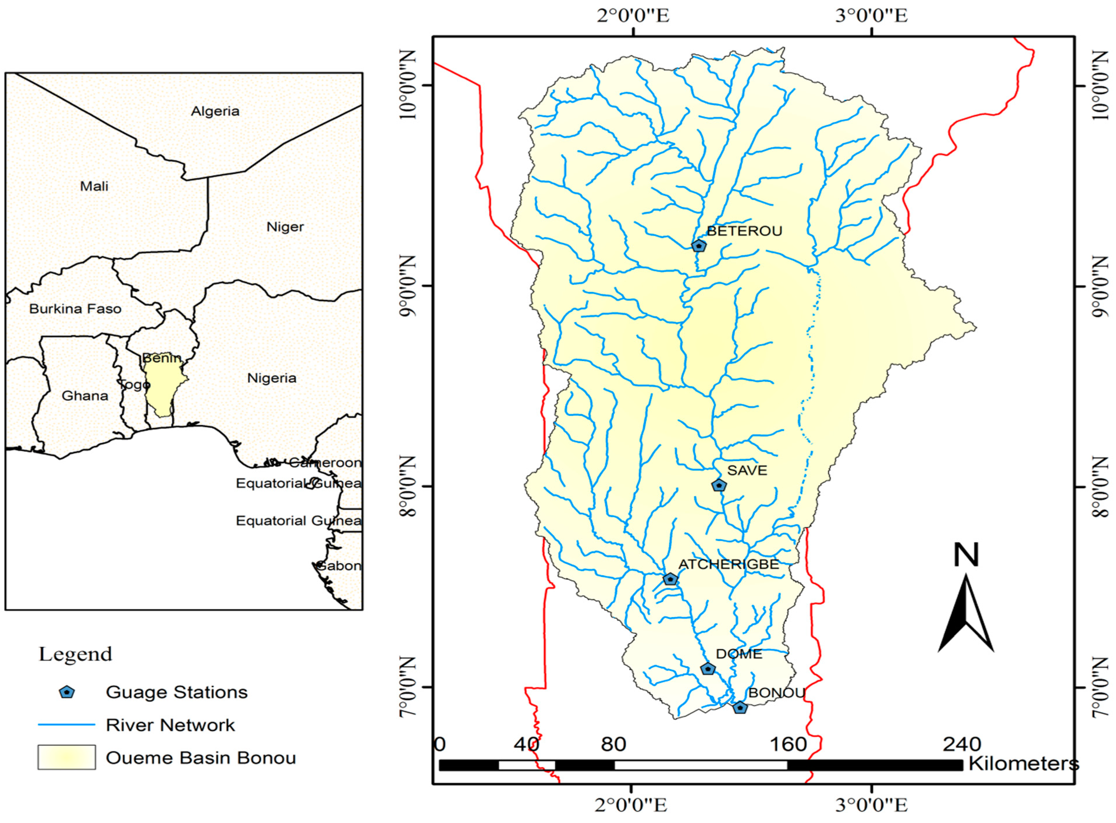
2.1. Study Area and Data
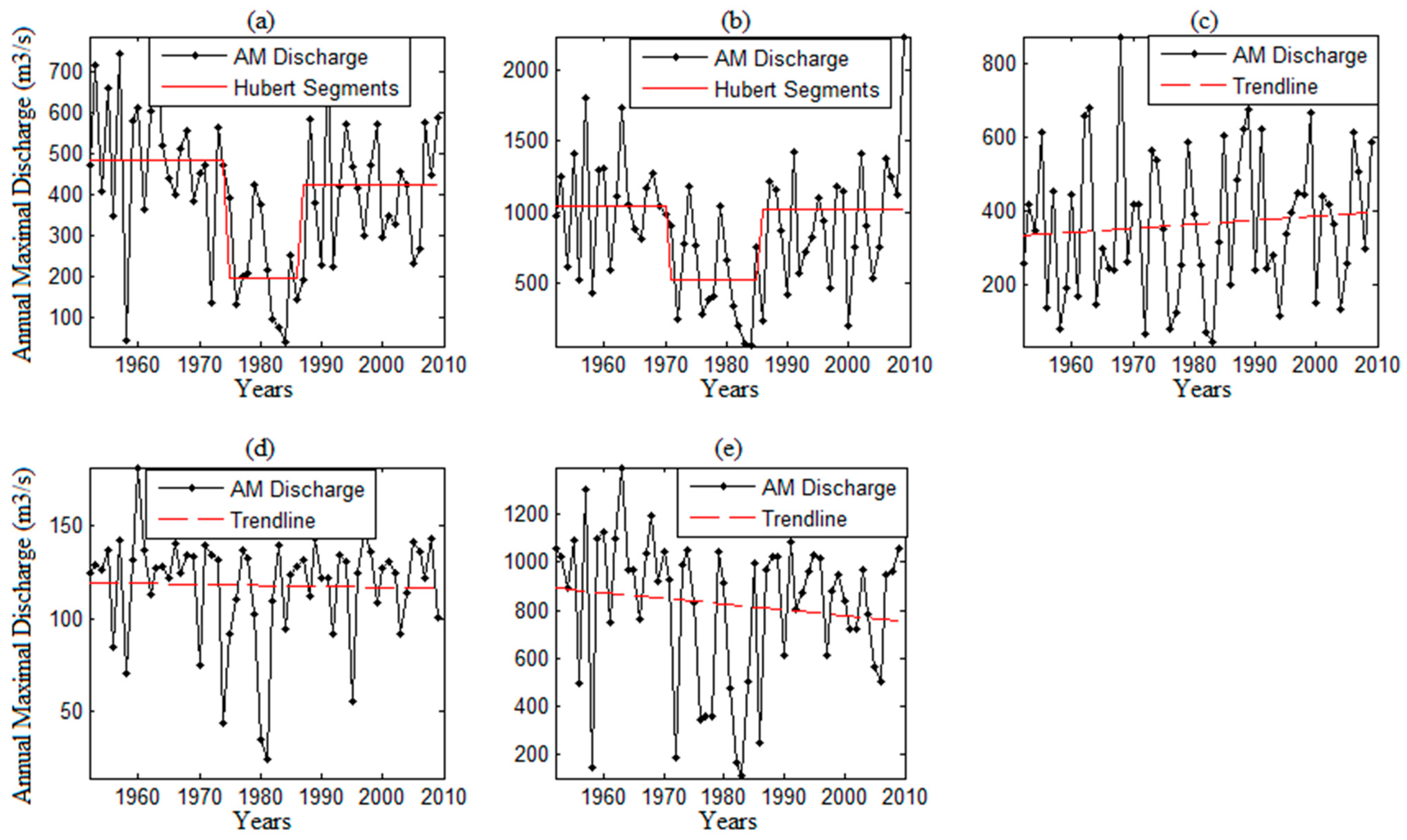
2.2. Preliminary Analysis
2.3. Climate Indexes

| Stations | Bonou | Bétérou | Savè | Atchérigbé | Domè |
|---|---|---|---|---|---|
| SST or SLP | SLP | SLP | SLP | SST | SST |
| Period | Annual Average | Annual Average | August | July | August |
| Longitude | 357° | 357° | 357° | 351° | 3° |
| Latitude | −4° | −4° | −4° | −4° | 4° |
| Correlation coefficient | −0.6 | −0.6 | −0.5 | 0.6 | −0.3 |
2.4. Method for Modeling Extreme Stream Flows
| Models | Location Parameter | Scale Parameter | Shape Parameter |
|---|---|---|---|
| GEV-0 | μ = constant | σ = constant | κ = constant |
| GEV-1 | μ(t) = μ0 + μ1*Cov(t) | σ = constant | κ = constant |
| GEV-2 | μ(t) = μ0 + μ1*Cov(t) | log(σ) = σ0+ σ1*Cov(t) | κ = constant |
| GEV-3 | μ(t) = μ0 + μ1*t | σ = constant | κ = constant |
| GEV-4 | μ(t) = μ0 + μ1*t | log(σ) = σ0 + σ1*t | κ = constant |
| GEV-5 | μ(t) = μ0 + μ1*t + μ2*Cov(t) | σ = constant | κ = constant |
| GEV-6 | μ(t) = μ0 + μ1*Cov(t) | log(σ) = σ0+ σ 1*t | κ = constant |
3. Results and Discussions
| Model | GEV-0 | GEV-1 | GEV-2 | GEV-3 | GEV-4 | GEV-5 | GEV-6 |
|---|---|---|---|---|---|---|---|
| Atchérigbé | ns | 1 | ns | ns | ns | 2 | 3 |
| Bétérou | 3 | 1 | ns | ns | ns | 2 | ns |
| Bonou | 3 | 1 | ns | ns | ns | 2 | ns |
| Domè | 2 | 1 | ns | ns | ns | ns | ns |
| Savè | 4 | 1 | ns | ns | ns | 2 | 3 |
| Stations | Models | Location | Scale | Shape | Performance Criteria | |||||
|---|---|---|---|---|---|---|---|---|---|---|
| μ0(Δμ0) | μ1(Δμ1) | σ0(Δσ0) | κ(Δ κ) | −ln(L) | Deviance Statistic | p-value | AIC | BIC | ||
| Atchérigbé | GEV-14par. | 317.7 (22.5) | 148.0 (28.8) | 151.2 (16.1) | −0.2 (0.1) | 375.7 | 22.1 | 3e−06 | 759.5 | 767.7 |
| Bétérou | GEV-1 | 347.5 (21.2) | −270 (49.3) | 149.6 (14.7) | −0.3 (0.1) | 370.3 | 26.3 | <1e−06 | 748.6 | 756.9 |
| Bonou | GEV-1 | 749.2 (36.8) | −389 (75.7) | 259.7 (27.0) | −0.5 (0.1) | 398.5 | 23.7 | 1e−06 | 805.0 | 813.2 |
| Domè | GEV-1 | 122.6 | −24.6 | 34.2 | −1.2 | 260.1 | 29.6 | <1e−06 | 528.2 | 536.5 |
| Savè | GEV-1 | 812.4 (57.7) | −357 (88.5) | 374.2 (36.1) | −0.2 (0.1) | 426.8 | 17.1 | 3.5e−05 | 861.6 | 869.8 |
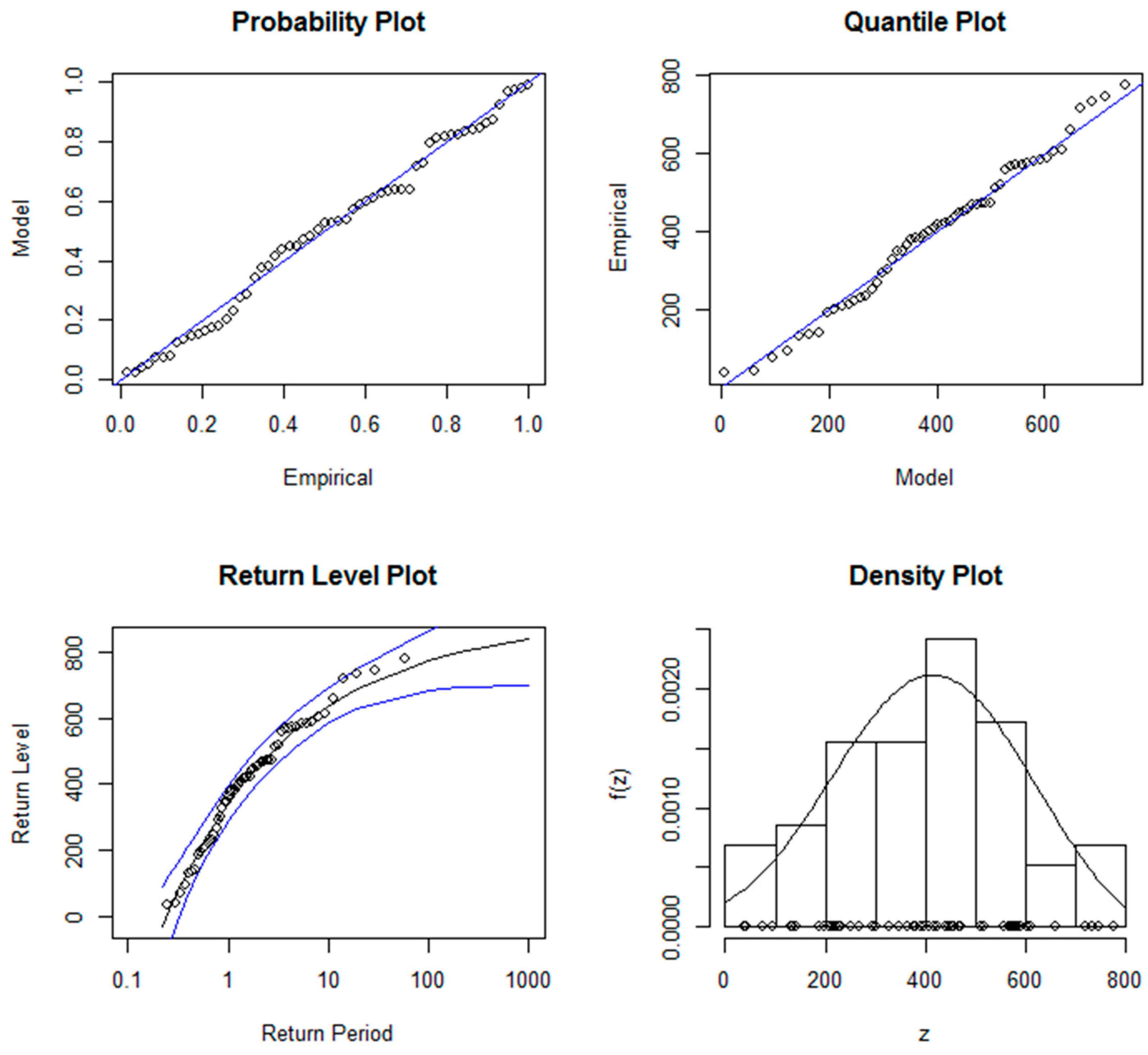
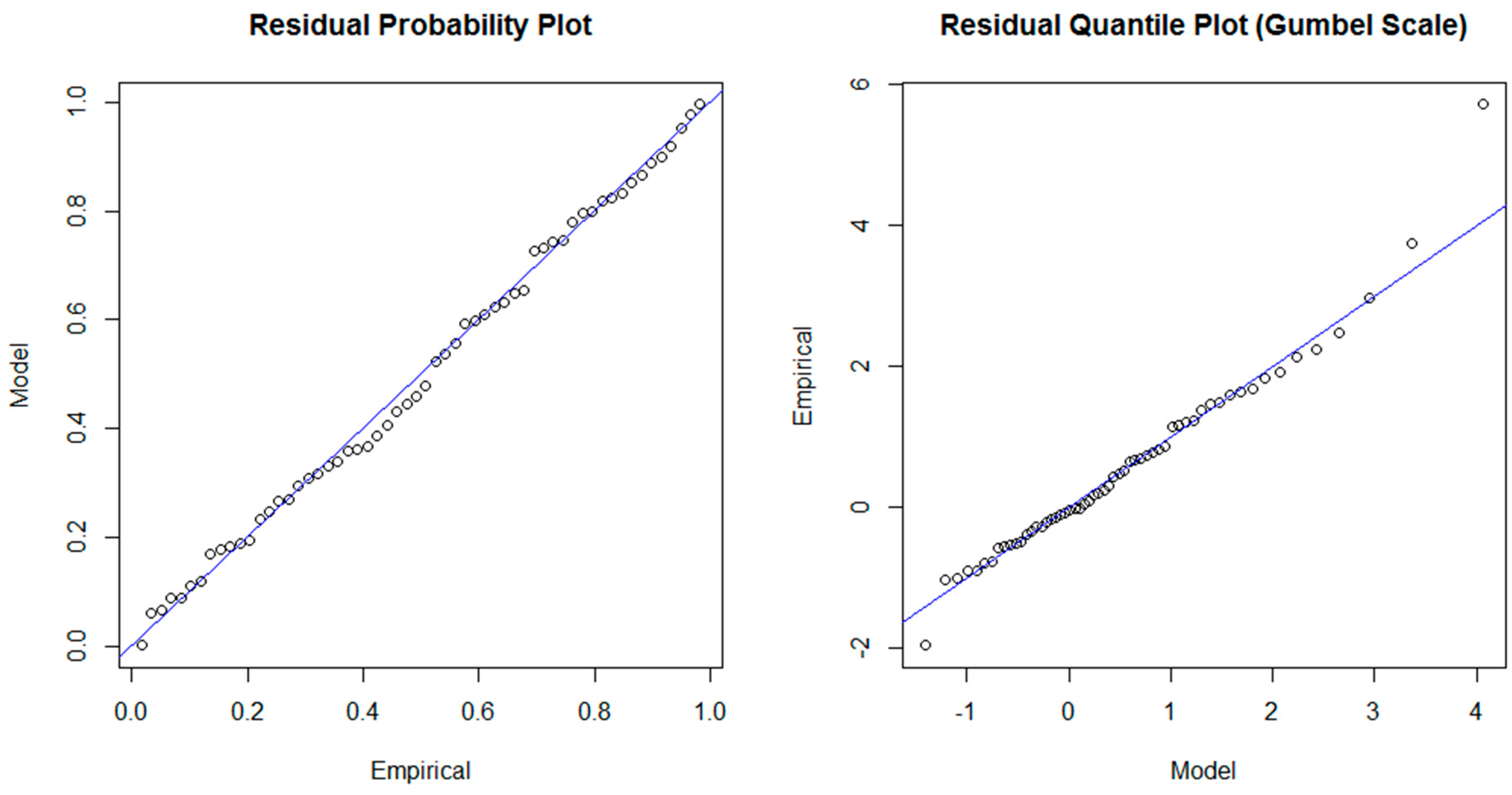
3.1. GEV-1 Model
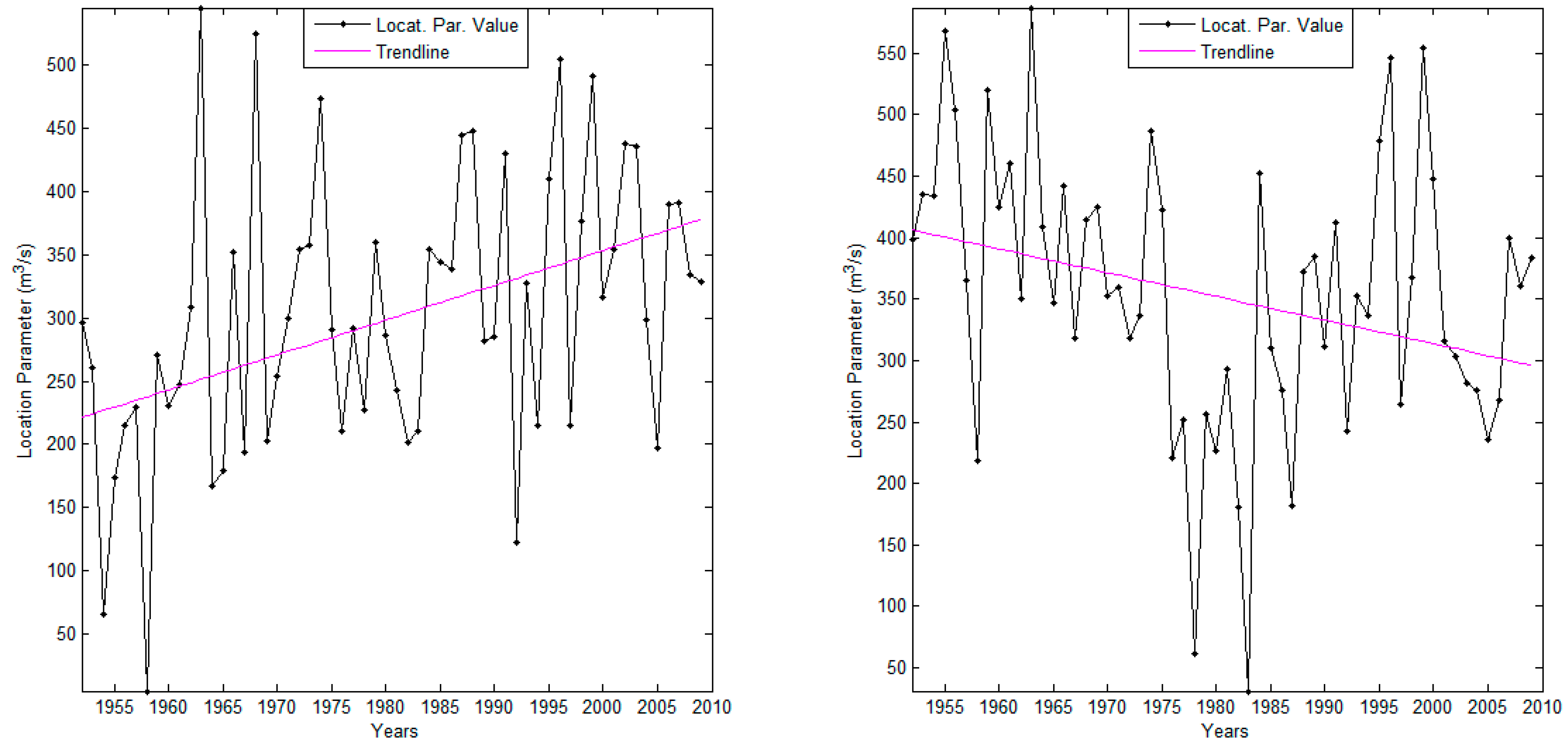
3.2. Non-Stationarity in the Location Parameter

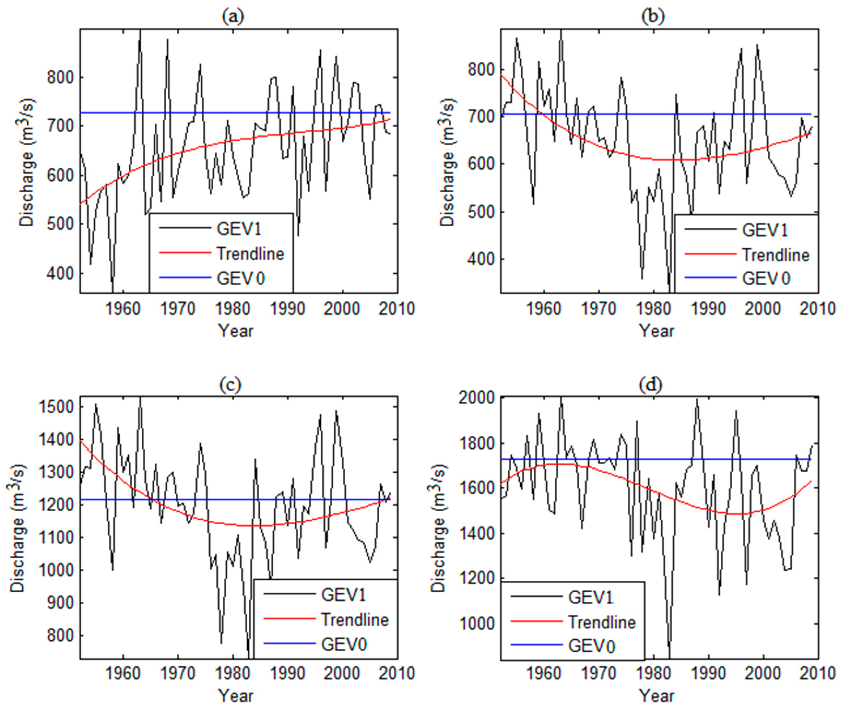
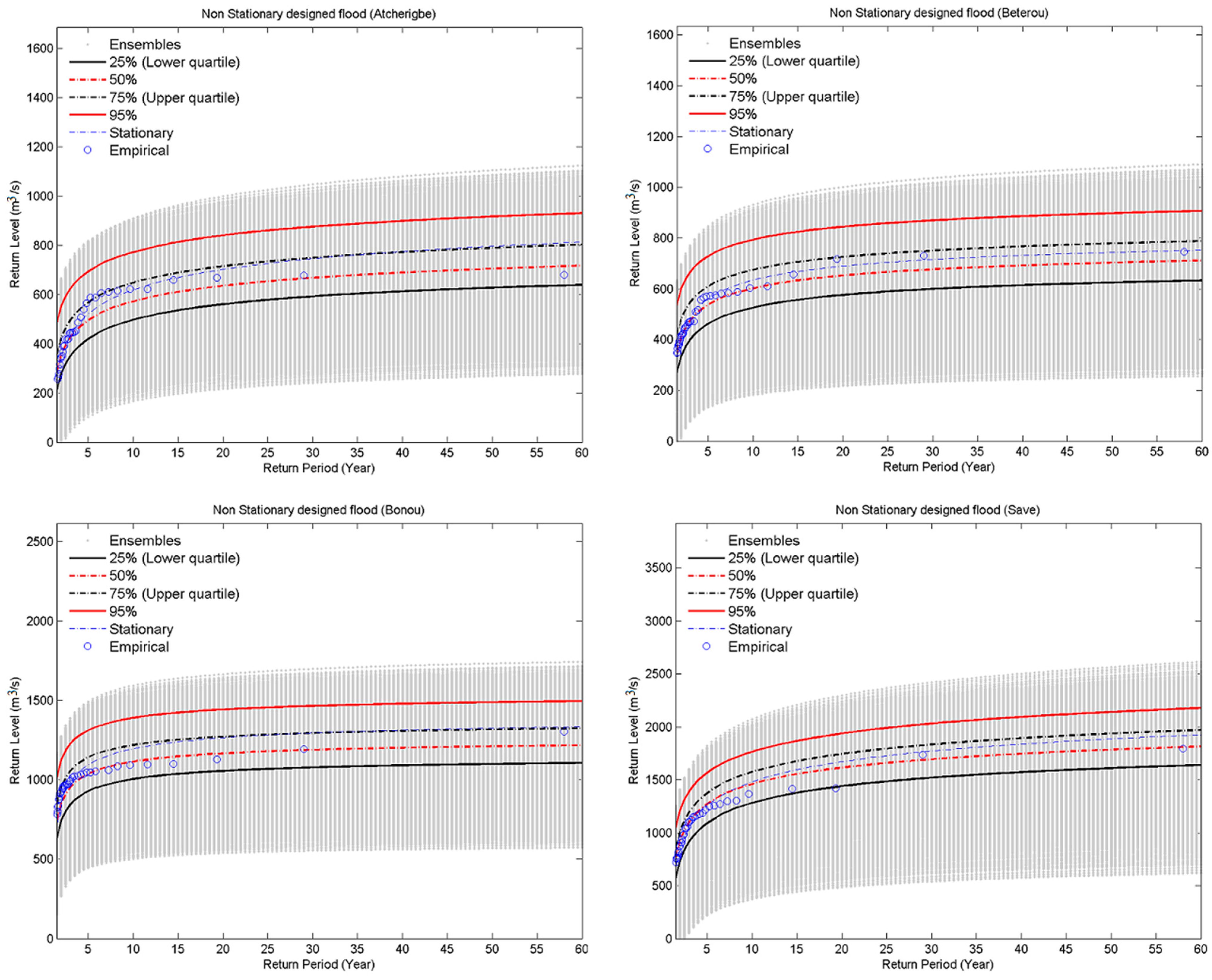
3.3. Stationary and Non-Stationary Effective Return Level Estimation

3.4. Non-Stationary Design Values Estimation
| Return Period | 2 | 5 | 10 | 15 | 25 | 30 | 40 | 45 | 50 | 60 | Risk Level |
|---|---|---|---|---|---|---|---|---|---|---|---|
| Non-stationary return level | |||||||||||
| Atchérigbé | 353 | 495 | 572 | 635 | 653 | 667 | 689 | 697 | 704 | 717 | High Risk |
| 423 | 567 | 648 | 714 | 734 | 749 | 772 | 781 | 789 | 802 | Medium Risk | |
| 551 | 693 | 772 | 840 | 860 | 875 | 898 | 908 | 916 | 930 | Low Risk | |
| Bétérou | 408 | 537 | 602 | 652 | 666 | 676 | 692 | 698 | 703 | 711 | High Risk |
| 480 | 610 | 674 | 725 | 739 | 750 | 767 | 773 | 779 | 788 | Medium Risk | |
| 599 | 728 | 793 | 844 | 858 | 869 | 886 | 892 | 897 | 907 | Low Risk | |
| Bonou | 849 | 1037 | 1114 | 1166 | 1179 | 1189 | 1202 | 1207 | 1211 | 1218 | High Risk |
| 953 | 1141 | 1219 | 1272 | 1285 | 1294 | 1308 | 1313 | 1317 | 1324 | Medium Risk | |
| 1123 | 1311 | 1390 | 1443 | 1456 | 1465 | 1479 | 1484 | 1489 | 1496 | Low Risk | |
| Savè | 922 | 1270 | 1459 | 1614 | 1658 | 1693 | 1745 | 1766 | 1784 | 1814 | High Risk |
| 1014 | 1372 | 1573 | 1743 | 1793 | 1833 | 1892 | 1915 | 1936 | 1970 | Medium Risk | |
| 1210 | 1565 | 1763 | 1936 | 1988 | 2031 | 2092 | 2118 | 2139 | 2178 | Low Risk | |
| Stationary return level | |||||||||||
| Atchérigbé | 348 | 521 | 619 | 702 | 726 | 745 | 774 | 786 | 796 | 813 | |
| Bétérou | 406 | 560 | 634 | 689 | 704 | 716 | 732 | 738 | 743 | 752 | |
| Bonou | 853 | 1094 | 1195 | 1265 | 1282 | 1295 | 1313 | 1320 | 1326 | 1335 | |
| Savè | 851 | 1253 | 1480 | 1671 | 1727 | 1771 | 1837 | 1863 | 1886 | 1924 | |
4. Conclusions
Acknowledgments
Author Contributions
Conflict of Interest
References and Notes
- EM-DAT The OFDA/CRED International Disaster Database. Available online: http://www.emdat.be (accessed on 23 September 2013).
- Amoussou, E.; Tramblay, Y.; Totin, H.S.V.; Mahé, G.; Camberlin, P. Dynamics and modelling of floods in the river basin of Mono in Nangbeto, Togo/Benin. Hydrol. Sci. J. 2014, 59, 2060–2071. [Google Scholar] [CrossRef]
- Di Baldassarre, G.; Montanari, A.; Lins, H.; Koutsoyiannis, D.; Brandimarte, L.; Blöschl, G. Flood fatalities in Africa: From diagnosis to mitigation. Geophys. Res. Lett. 2010. [Google Scholar] [CrossRef]
- World Meteorological Organization (WMO). Flood Management in a Changing Climate: A Tool for Integrated Flood Management. Available online: http://www.apfm.info/publications/tools/Tool_09_FM_in_a_changing_climate.pdf (accessed on 13 October 2013).
- Goula, B.T.A.; Soro, E.G.; Kouassi, W.; Srohourou, B. Tendances et ruptures au niveau des pluies journalières extrêmes en Côte d ’ Ivoire (Afrique de l ’ Ouest). Hydrol. Sci. J. 2011, 57, 1067–1080. (In French) [Google Scholar] [CrossRef]
- Sighomnou, D.; Descroix, L.; Genthon, P.; Gil, M.; Emmanuele, G. La crue de 2012 a Niamey : un paroxysme du paradoxe du Sahel? Secheresse 2013, 24, 3–13. (In French) [Google Scholar]
- Nchito, W.S. Flood risk in unplanned settlements in Lusaka. Environ. Urban. 2007, 19, 539–551. [Google Scholar] [CrossRef]
- Kunkel, K.E.; Carolina, N. North American Trends in Extreme Precipitation. Nat. Hazards 2003, 29, 291–305. [Google Scholar] [CrossRef]
- Re, M.; Barros, V.R. Extreme rainfalls in SE South America. Clim. Change 2009, 96, 119–136. [Google Scholar] [CrossRef]
- Kiang, J.; Rolf, O.; Waskom, R. Workshop on Nonstationarity, Hydrologic Frequency Analysis, and Water Management. Available online: http://www.usbr.gov/research/climate/Workshop_ Nonstat.pdf (accessed on 5 July 2013).
- Brown, S.J.; Caesar, J.; Ferro, C.T. Global changes in extreme daily temperature since 1950. J. Geophys. Res. 2008. [Google Scholar] [CrossRef]
- Katz, R.W.; Parlange, M.B.; Naveau, P. Statistics of extremes in hydrology. Adv. Water Resour. 2002, 25, 1287–1304. [Google Scholar] [CrossRef]
- Aissaoui-Fqayeh, I.; El-Adlouni, S.; Ouarda, T.B.M.J.; St-Hilaire, A. Développement du modèle log-normal non-stationnaire et comparaison avec le modèle GEV non-stationnaire. Hydrol. Sci. J. 2009, 54, 1141–1156. (In French) [Google Scholar] [CrossRef]
- Tramblay, Y.; Neppel, L.; Carreau, J.; Kenza, N. Non-stationary frequency analysis of heavy rainfall events in Southern France. Hydrol. Sci. J. 2013, 58, 1–15. [Google Scholar] [CrossRef]
- Tramblay, Y.; Amoussou, E.; Dorigo, W.; Mahé, G. Flood risk under future climate in data sparse regions: Linking extreme value models and flood generating processes. J. Hydrol. 2014, 519, 549–558. [Google Scholar] [CrossRef]
- Alamou, E. Application du Principe de Moindre Action à la Modélisation Pluie-débit. Ph.D. Thesis, Université d’Abomey-Calavi, Abomey Calavi, Benin, 2011. [Google Scholar]
- Avahounlin, F.R.; Lawin, A.E.; Alamou, E.; Chabi, A.; Afouda, A. Analyse Fréquentielle des Séries de Pluies et Débits Maximaux de L’ ouémé et Estimation des Débits de Pointe. Eur. J. Sci. Res. 2013, 107, 355–369. (In French) [Google Scholar]
- Lopez, J.; Frances, F. Non-stationary flood frequency analysis in continental Spanish rivers, using climate and reservoir indices as external covariates. Hydrol. Earth Syst. Sci. 2013, 10, 3103–3142. [Google Scholar] [CrossRef]
- Sugahara, S.; Porfirio, R.; Silveira, R. Non-stationary frequency analysis of extreme daily rainfall in Sao Paulo, Brazil. Int. J. Climatol. 2009, 1349, 1339–1349. [Google Scholar] [CrossRef]
- Hanel, M.; Buishand, T.A.; Ferro, C.A.T. A non-stationary index-flood model for precipitation extremes in transient Regional Climate Model simulations. J. Geophys. Res. Atmos. 2009, 114, 1–61. [Google Scholar] [CrossRef]
- Khaliq, M.N.; Ha, C. Frequency analysis of a sequence of dependent and/or non-stationary hydro-meteorological observations: A review. J. Hydrol. 2006, 329, 534–552. [Google Scholar] [CrossRef]
- Osorio, J.D.G.; Galiano, S.G.G. Non-stationary analysis of dry spells in monsoon season of Senegal River Basin using data from Regional Climate Models (RCMs). J. Hydrol. 2012, 450-451, 82–92. [Google Scholar] [CrossRef]
- El-Adlouni, S.; Ouarda, T. Comparaison des méthodes d’estimation des paramètres du modèle GEV non stationnaire. Rev. des Sci. l’eau 2008, 21, 35–50. (In French) [Google Scholar] [CrossRef] [Green Version]
- Zenoni, E.; Pecora, S.; de Michele, C.; Vezzoli, R. Maximum Annual Flood Peaks Distribution in non-Stationary Conditions. In Comprehensive Flood Risk Management Research for Policy and Practice; Schweckendiek, T., Ed.; Taylor and Francis Group: London, UK, 2013. [Google Scholar]
- Conway, D.; Mah, G. River flow modelling in two large river basins with non-stationary behaviour : The Paraná and the Niger. 2009, 23, 3186–3192. [Google Scholar] [CrossRef]
- Rath, A.B.; Astellarin, A.C.; Ontanari, A.M. Detecting non-Stationarity in Extreme Rainfall Data Observed in Northern Italy. Available online: http://www.idrologia.polito.it/~claps/pliniusonline/pdf_proceedings/Plinius/Brath1/BRATH1.pdf (accessed on 27 October 2014).
- Ribereau, P.; Guillou, A.; Naveau, P. Estimating return levels from maxima of non-stationary random sequences using the Generalized PWM method. Nonlin. Processes Geophys. 2008, 15, 1033–1039. [Google Scholar] [CrossRef]
- Kharim, V.V.; Zwiers, F.W. Estimating Extremes in Transient Climate Change Simulations. J. Clim. 2004, 18, 1156–1173. [Google Scholar] [CrossRef]
- Coles, S.; Davison, A. Statistical Modelling of Extreme Values. Available online: http://www.cces.ethz.ch/projects/hazri/EXTREMES/talks/colesDavisonDavosJan08.pdf (accessed on 4 Feburary 2013).
- Fink, A.; Christoph, M.; Born, K.; Bruecher, T.; Piecha, K.; Pohle, S.; Schulz, O.; Ermert, V. Climate. In Impacts of Global Change on the Hydrological Cycle in West and Northwest Africa; Speth, P., Christoph, M., Diekkrüger, B., Eds.; Springer: Heidelberg, Germany, 2010. [Google Scholar]
- Deng, Z. Vegetation Dynamics in Oueme Basin, Benin, West Africa; Cuvillier Verlag: Göttingen, Germany, 2007. [Google Scholar]
- Diekkrüger, B.; Busche, H.; Giertz, S.; Steup, G. Hydrology. In Impacts of Global Change on the Hydrological Cycle in West and Northwest Africa; Speth, P., Christoph, M., Diekkrüger, B., Eds.; Springer: Heidelberg, Germany, 2010. [Google Scholar]
- Robson, A.J.; Jones, T.K.; Reed, D.W.; Bayliss, A.C. A study of national trend and variation in UK floods. Int. J. Climatol. 1998, 18, 165–182. [Google Scholar] [CrossRef]
- Xiong, L.; Guo, S. Trend test and change-point detection for the annual discharge series of the Yangtze River at the Yichang hydrological station. Hydrol. Sci. 2004, 49, 99–112. [Google Scholar] [CrossRef]
- Pettitt, A.N. A Non-Parametric Approach to the Change-Point Problem. J. R. Stat. Soc. Ser. C. Appl. Stat. 1979, 28, 126–135. [Google Scholar] [CrossRef]
- Hubert, P.; Carbonnel, J.P.; Chaouche, A. Segmentation des séries hydrométéorologiques—Application à des séries de précipitations et de débits de l’afrique de l'ouest. J. Hydrol. 1989, 110, 349–367. (In French) [Google Scholar] [CrossRef]
- Servat, E.; Paturel, J.E.; Lubes-Niel, H.; Kouamé, B.; Masson, J.M.; Travaglio, M.; Marieu, B. De différents aspects de la variabilité de la pluviométrie en Afrique de l’ouest et centrale non sahélienne. Rev. des Sci. l’eau 1999, 12, 363–387. (In French) [Google Scholar] [CrossRef]
- Vissin, E.; Boko, M.; Houndenou, C.; Perard, J. Recherche de ruptures dans les séries pluviométriques et hydrologiques du bassin beninois du fleuve niger (Bénin, Afrique de l’ouest). Available online: http://www.climato.be/aic/colloques/actes/PubAIC/art_2003_vol15/Article% 2045 E Vissin.pdf (accessed on 5 August 2013). (In French)
- Detecting Trend And Other Changes In Hydrological Data. Available online: http://water.usgs.gov/osw/wcp-water/detecting-trend.pdf (accessed on 23 September 2013).
- Jain, S.; Lall, U. Floods in a changing climate: does the past represent the future? Water Resour. Res. 2001, 37, 3193–3205. [Google Scholar] [CrossRef]
- McKerchar, M.E.; Moss, C.P.; Pearson, A. The Southern Oscillation index as a predictor of the probability of low streamflows in New Zealand. Water Resour. Res. 1994, 30, 2717–2723. [Google Scholar]
- Yang, C.; Hill, D. Modeling Stream Flow Extremes under Non-Time-Stationary Conditions. Available online: http://cmwr2012.cee.illinois.edu/Papers/Special%20Sessions/Data-driven%20Approaches%20for%20Water%20Resources%20Forecasting%20and%20Knowledge/Yang_Ci_CMWR2012_Final%20version.pdf (accessed on 3 September 2014).
- Mitchell, T. 4 by 6-Degree Latititude-Longitude Resolution Anomalies of ICOADS SST, SLP, Surface Air Temperature, Winds, and Cloudiness. Available online: http://jisao.washington.edu/data_sets/sstanom_4by6/ (accessed on 17 July 2014).
- Janicot, S.; Thorncroft, C.D.; Ali, A.; Asencio, N.; Berry, G.; Bock, O.; Bourles, B.; Caniaux, G.; Chauvin, F.; Deme, A.; et al. Large-scale overview of the summer monsoon over West Africa during the AMMA field experiment in 2006. Ann. Geophys. 2008, 26, 2569–2595. [Google Scholar] [CrossRef]
- Janicot, S.; Ali, H.; Fontaine, B.; Vincent, M. West African Monsoon Dynamics and Eastern Equatorial Atlantic and Pacific SST Anomalies (1970–88). J. Clim. 1998, 11, 1874–1883. [Google Scholar] [CrossRef]
- Losada, T.; Rodriguez-Fonseca, B.; Janicot, S.; Gervois, S.; Chauvin, F.; Ruti, P. A multimodel approach to the Atlantic ecuatorial mode. Impact on the West African monsoon. Clim. Dyn. 2010, 35, 29–43. [Google Scholar] [CrossRef]
- Coles, S. An Introduction to Statistical Modeling of Extreme Values; Springer: Bristol, UK, 2001. [Google Scholar]
- Markose, S.; Alentorn, A. The Generalized Extreme Value (GEV) Distribution, Implied Tail Index and Option Pricing. J. Deriv. 2011, 18, 35–60. [Google Scholar] [CrossRef]
- Hounkpè, J.; Afouda, A.A.; Diekkrüger, B.; Hountondji, F. Modelling extreme streamflows under non-stationary conditions in Ouémé river basin, Benin, West Africa. In Hydrological Sciences and Water Security: Past, Present and Future; IAHS (International Association of Hydrological Sciences): Paris, France, 2015; pp. 143–144. [Google Scholar]
- R Development Core Team. R: A Language and Environment for Statistical Computing; R Foundation for Statistical Computing: Vienna, Austria, 2009. [Google Scholar]
- Gilleland, E.; Katz, R.W. Extremes Toolkit (extRemes): Weather and Climate Applications of Extreme Value. Available online: www.isse.ucar.edu/extremevalues/extreme.pdf (accessed on 23 December 2014).
- Akaike, H. A New Look at the Statistical Model Identification. IEEE Trans. Autom. Control 1974, 19, 716–723. [Google Scholar] [CrossRef]
- Schwarz, G. Estimating the Dimension of a Model. Ann. Stat. 1978, 6, 461–464. [Google Scholar] [CrossRef]
- McKay, M.D.; Beckman, R.J.; Conover, W.J. A comparison of three methods for selecting values of input variables in the analysis of output from a computer code. Technometrics 2000, 42, 55–61. [Google Scholar] [CrossRef]
- Cheng, L.; Aghakouchak, A.; Gilleland, E.; Katz, R.W. Non-stationary extreme value analysis in a changing climate. Clim. Change 2014, 127, 353–369. [Google Scholar] [CrossRef]
- Sen, P.K. Estimates of the Regression Coefficient Based on Kendall’s Tau. J. Am. Stat. Assoc. 1968, 63, 1379–1389. [Google Scholar] [CrossRef]
- Philippon, N. Une nouvelle approche pour la prévision statistique des précipitations saisonnières en Afrique de l’ Ouest et de l'est: méthodes, diagnostics et application. Available online: http://climatologie.u-bourgogne.fr/perso/nphilipp/thesis/Thesis.pdf (accessed on 27 March 2014). (In French)
- Di Baldassarre, G.; Claps, P. A hydraulic study on the applicability of flood rating curves. Hydrol. Res. 2010. [Google Scholar] [CrossRef]
- World Bank. Inondation au Benin: Rapport d’evaluation des Besoins Post Catastrophe. Available online: http://www.gfdrr.org/sites/gfdrr.org/files/GFDRR_Benin_PDNA_2010.pdf (access on 1 December 2013). (In French)
© 2015 by the authors; licensee MDPI, Basel, Switzerland. This article is an open access article distributed under the terms and conditions of the Creative Commons Attribution license (http://creativecommons.org/licenses/by/4.0/).
Share and Cite
Hounkpè, J.; Diekkrüger, B.; Badou, D.F.; Afouda, A.A. Non-Stationary Flood Frequency Analysis in the Ouémé River Basin, Benin Republic. Hydrology 2015, 2, 210-229. https://doi.org/10.3390/hydrology2040210
Hounkpè J, Diekkrüger B, Badou DF, Afouda AA. Non-Stationary Flood Frequency Analysis in the Ouémé River Basin, Benin Republic. Hydrology. 2015; 2(4):210-229. https://doi.org/10.3390/hydrology2040210
Chicago/Turabian StyleHounkpè, Jean, Bernd Diekkrüger, Djigbo F. Badou, and Abel A. Afouda. 2015. "Non-Stationary Flood Frequency Analysis in the Ouémé River Basin, Benin Republic" Hydrology 2, no. 4: 210-229. https://doi.org/10.3390/hydrology2040210
APA StyleHounkpè, J., Diekkrüger, B., Badou, D. F., & Afouda, A. A. (2015). Non-Stationary Flood Frequency Analysis in the Ouémé River Basin, Benin Republic. Hydrology, 2(4), 210-229. https://doi.org/10.3390/hydrology2040210