Abstract
This study investigates how a Long Short-Term Memory (LSTM) model internally represents baseflow contributions in snowmelt-driven, semi-arid mountain basins with heterogeneous geologic characteristics. Five basins in the Sangre de Cristo Mountains of northern New Mexico, spanning fractured Precambrian bedrock and sedimentary-volcanic terrain, were used to evaluate both model performance and interpretability. Baseflow dynamics were inferred post hoc using the Baseflow Index (BFI) and a two-reservoir HEC-HMS (Hydrologic Engineering Center’s Hydrologic Modeling System) model. Although baseflow components were not explicitly included in model training, internal cell state activations exhibited strong correlations with both shallow and deep baseflow components derived from the HEC-HMS model. To better understand how these relationships may change under climatic stress, BFI-based baseflow patterns were further analyzed under pre-drought and drought conditions. Results indicate that the internal LSTM states differentiated patterns consistent with short- and long-residence flow paths, reflecting physically interpretable hydrologic behavior. This work demonstrates the potential of LSTM models to provide valuable insights into baseflow generation and groundwater–surface water interactions, which is especially critical in water-scarce regions facing increasing drought frequency.
1. Introduction
Mountain regions play a critical role in global water security, supplying freshwater to nearly half of the world’s population while occupying a disproportionately small fraction of the Earth’s land surface. As natural “water towers,” mountainous catchments regulate the timing and magnitude of downstream water availability through seasonal snow accumulation, delayed melt, and subsurface storage processes [1]. Climate change is increasingly altering these dynamics through shifts in precipitation phase, declining snowpack, earlier snowmelt, and more frequent and severe droughts, with well-documented impacts on summer streamflow in snow-dominated basins [2,3]. As seasonal snowmelt contributions decline or shift earlier in the year, groundwater discharge becomes increasingly important for sustaining streamflow during late summer and fall low-flow periods [4,5]. Accurately representing groundwater–surface water interactions is therefore fundamental to understanding and managing water resources in mountain regions under ongoing climatic change.
Groundwater flow in mountain systems is governed by complex and often poorly observed subsurface processes, including fractured bedrock flow paths, deep mountain-block aquifers, and long residence times that span months to decades [1,3,6,7,8,9,10,11]. Recent hydrogeologic studies have demonstrated that groundwater circulation in mountain catchments extends well beyond shallow soil layers, with substantial storage and delayed release occurring within fractured crystalline bedrock and deeper subsurface systems [6,7,8,9]. These deeper flow paths can buffer streamflow during prolonged dry periods and sustain baseflow well after seasonal snowmelt has ceased, particularly in semi-arid regions [2,8,11,12]. However, because these processes are largely hidden from direct observation and difficult to constrain with available data, their representation in hydrologic models remains a major challenge. Although physically based models offer conceptual transparency, they often struggle to capture the full spectrum of groundwater storage and release behavior at basin scales, especially under changing climatic conditions and limited subsurface data [13,14,15,16].
In contrast, data-driven models—particularly Long Short-Term Memory (LSTM) neural networks—have demonstrated strong predictive skill for streamflow simulation across a wide range of hydroclimatic regimes, including snowmelt-dominated mountain basins [17,18,19,20]. LSTMs are well suited for hydrologic applications because their recurrent architecture enables them to learn temporal dependencies, antecedent conditions, and delayed responses without explicit process prescriptions [21,22,23]. As a result, LSTM internal states may develop latent representations statistically associated with subsurface storage and delayed groundwater contributions, even when such processes are not explicitly included during model training [22]. Despite their predictive success, however, LSTM models are often criticized as “black boxes,” as their internal representations are not directly interpretable and are not constrained by physical process formulations.
Advances in explainable artificial intelligence (XAI) have improved transparency in hydrologic machine learning by identifying influential inputs, nonlinear sensitivities, and attribution pathways [23,24,25,26]. While these approaches have advanced understanding of input–output relationships, they provide limited insight into how recurrent neural networks internally encode hydrologic memory, storage, and delayed release processes, particularly those associated with groundwater contributions [27,28]. Conversely, internal-state analysis directly examines the hidden and cell states of LSTM models, offering a complementary interpretability pathway that emphasizes emergent hydrologic behavior, temporal persistence, and memory dynamics rather than explicit attribution [27,28,29,30,31]. Recent studies have shown that internal LSTM states can encode physically meaningful signals related to storage, delay, and runoff generation, revealing aspects of model behavior that are not accessible through attribution-based XAI alone [22,27,28,29,30].
In the southwestern United States, mountain headwater basins play a critical role in sustaining regional water supplies, particularly in semi-arid environments where snowmelt-driven runoff and groundwater discharge jointly support perennial streams [14,32,33,34,35]. In these settings, groundwater circulates through both shallow and deep subsurface pathways, often within fractured Precambrian bedrock or heterogeneous sedimentary–volcanic formations, maintaining streamflow well beyond the snowmelt season [6,7]. Recent work has demonstrated that groundwater contributions in these mountain systems are more dynamically cycled and extend to greater depths than traditionally represented in conceptual or numerical models [6,7,8,9]. Yet, because deeper groundwater pathways remain poorly observed, their role in streamflow generation is often inferred indirectly through recession analysis, baseflow separation, or hydrochemical tracers rather than direct measurement [10].
While LSTM performance for streamflow prediction has received significant attention in recent years, relatively little work has examined whether—and to what extent—LSTM models internalize physically meaningful representations of groundwater storage and baseflow dynamics in geologically complex, snowmelt-dominated mountain basins. Existing interpretability studies have largely focused on large-sample datasets, runoff-dominated systems, or generic hydrologic memory metrics, with limited attention to groundwater-dominated headwaters where delayed subsurface contributions play a dominant role in drought resilience [23,26,36,37]. As a result, the extent to which LSTM internal memory states reflect physically meaningful groundwater behavior—such as fast versus slow subsurface flow paths or residence-time-controlled baseflow—remains poorly understood, especially in snowmelt-dominated systems where subsurface storage and release play a dominant role [23].
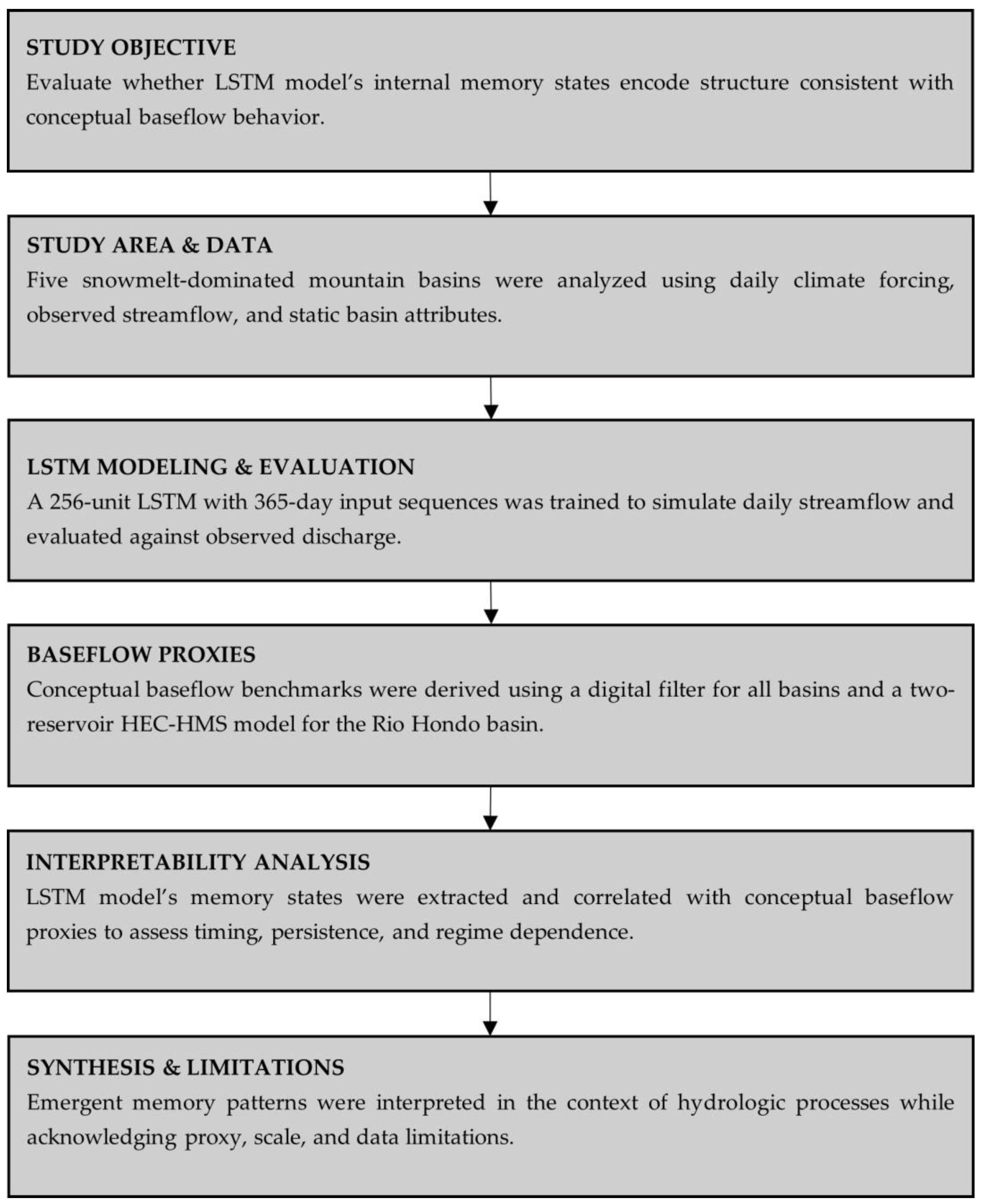
Building on recent work demonstrating that LSTM internal states can encode hydrologic processes without explicit supervision, this study applies internal-state analysis to snowmelt-dominated mountain basins where groundwater storage and delayed release are central to streamflow generation [22,31]. The overall study design and analysis workflow are summarized in Figure 1. Rather than treating the LSTM as a purely predictive tool, this study examines the model’s internal memory states to assess whether they encode structure consistent with conceptual baseflow behavior. Extracted LSTM cell and hidden states are compared to multiple independent, physically informed benchmarks, including digital baseflow separation, a two-reservoir HEC-HMS (Hydrologic Engineering Center’s Hydrologic Modeling System) model, and qualitative hydrochemical source classifications from a previously published end-member mixing analysis (EMMA) conducted in the same study area [35]. Importantly, baseflow information was not used during model training; all comparisons are performed post hoc to evaluate emergent internal behavior rather than prescribed process representation.
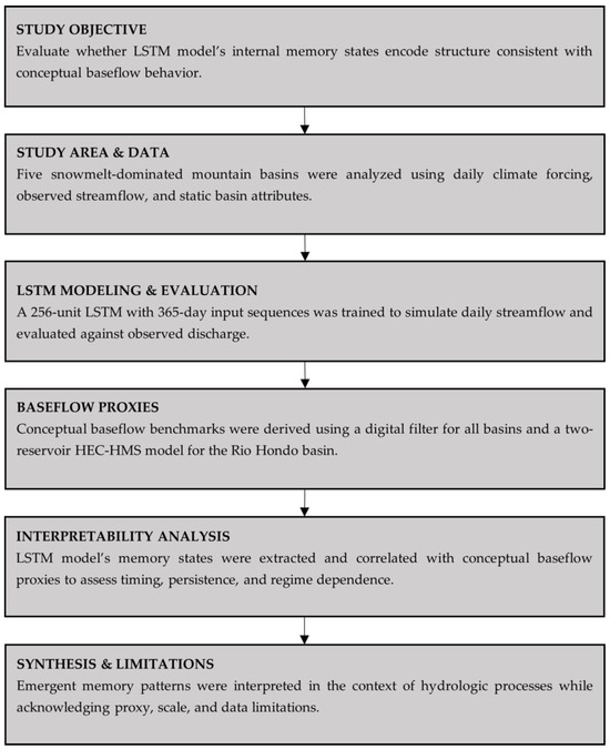
Figure 1.
Overview of the study workflow for evaluating internal LSTM states against conceptual baseflow behavior.
This study addresses the following research questions:
- (RQ1) Can LSTM models trained solely on meteorological and hydrologic inputs develop internal memory representations that are statistically and conceptually consistent with physically derived baseflow components in snowmelt-dominated mountain basins?
- (RQ2) Do distinct LSTM states preferentially align with fast and slow groundwater response regimes, as represented by conceptual baseflow models and independent hydrochemical classifications?
- (RQ3) How does the representation of baseflow-related memory states change under contrasting hydroclimatic conditions, particularly during extended drought periods when groundwater contributions dominate streamflow?
We hypothesize that the LSTM model’s internal memory states encode hydrologically meaningful information related to groundwater storage and delayed release and that these representations can be revealed through comparison with physically informed baseflow proxies and hydrochemical context. By focusing on internal-state behavior rather than predictive performance alone, this work advances hydrologic interpretability of machine learning models and provides new insight into groundwater–surface water interactions in snowmelt-dominated, semi-arid mountain environments.
2. Materials and Methods
2.1. Study Area
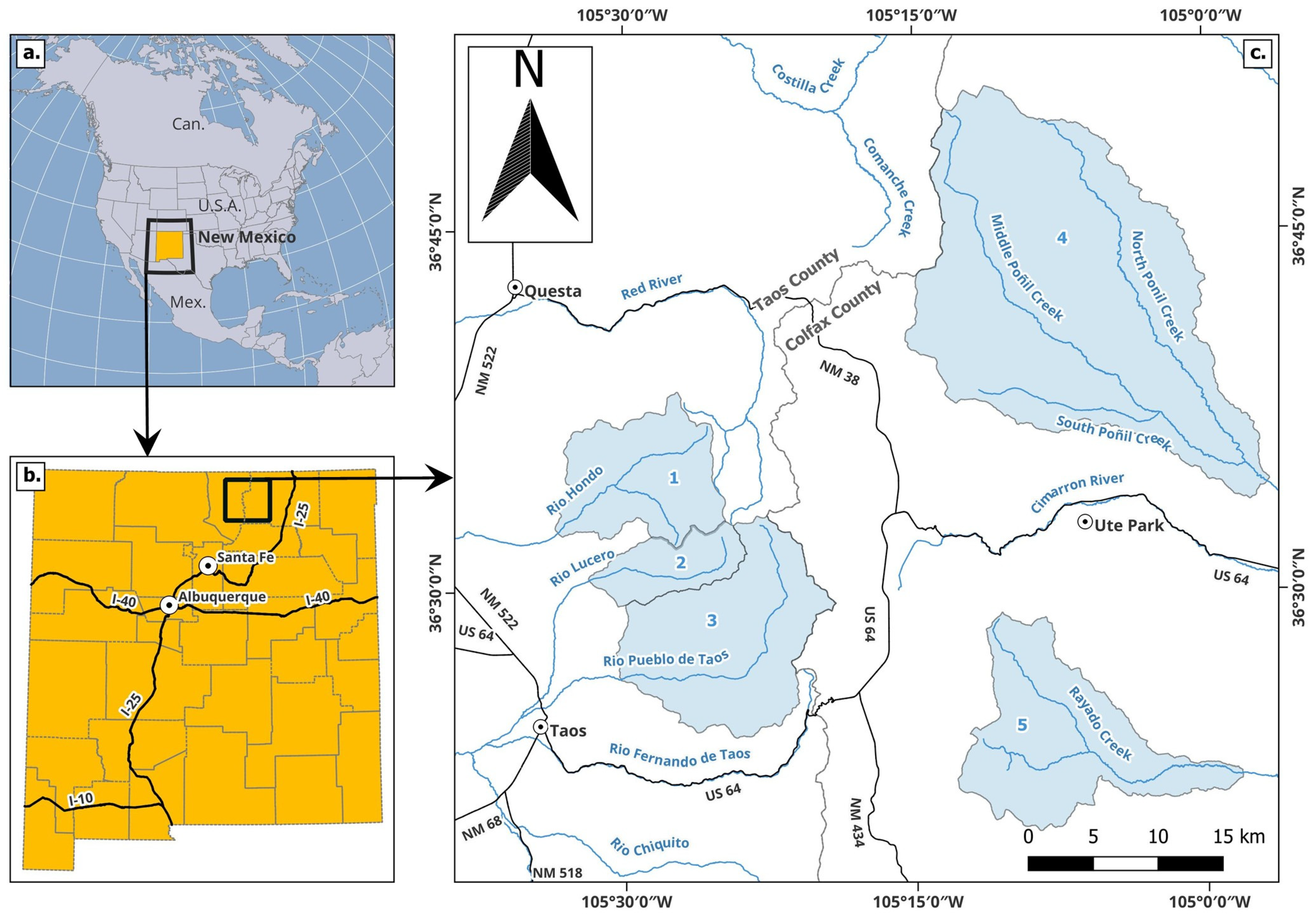
This study examines five river basins located in the Sangre de Cristo Mountains of northern New Mexico, near Taos (Figure 2). These include three basins in the Taos Range (Rio Hondo, Rio Lucero, and Rio Pueblo de Taos) and two in the Cimarron Range (Ponil Creek and Rayado Creek). The Taos and Cimarron Ranges, separated by the Moreno Valley, represent geologically distinct subranges of the Sangre de Cristo Mountains, with implications for groundwater storage and stream–aquifer interactions.
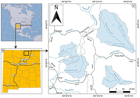
Figure 2.
Study area near Taos, New Mexico. Panel (a) shows the regional location within North America, panel (b) shows the location within New Mexico, and panel (c) depicts the five headwater basins used in this study: (1) Rio Hondo, (2) Rio Lucero, (3) Rio Pueblo de Taos, (4) Ponil Creek, and (5) Rayado Creek. Black lines indicate major roads, blue lines represent rivers and streams, and shaded blue polygons denote the study basins.
The Taos Range basins lie along the western flank of the Moreno Valley and drain into the Rio Grande. This range is dominated by Precambrian metamorphic rocks, including gneiss, schist, and granite, which are commonly fractured and faulted [38,39]. These features create opportunities for groundwater storage and delayed subsurface discharge that sustains baseflow during dry periods [6,7]. The Sangre de Cristo Fault, which borders the western margin of the range, contributes to a fault-block mountain structure with steep topography and deep valleys [40].
By contrast, the Cimarron Range basins drain eastward into the Canadian River system and are composed of Paleozoic and Mesozoic sedimentary rocks interspersed with Tertiary volcanic intrusions [41,42]. These formations are more erodible and less fractured than those in the Taos Range [41], resulting in smoother terrain and reduced potential for long-term groundwater storage [39]. Table 1 summarizes the location, physiographic, and hydroclimatic characteristics of the five study basins, providing context for differences in snow accumulation, temperature regime, and runoff generation across the study area.

Table 1.
Location, physiographic, and hydroclimatic characteristics of the study basins.
Across the five basins, basin-averaged mean annual precipitation ranges from approximately 531 to 656 mm yr−1, with snowfall comprising roughly 21–43% of annual precipitation, reflecting strong elevation influences across the study area. Mean annual air temperatures range from approximately 2.2 to 5.7 °C, consistent with pronounced elevation gradients and prolonged winter snow accumulation in the higher-elevation basins.
The five study basins were selected to provide a controlled yet contrasting set of snowmelt-dominated mountain catchments suitable for evaluating internal hydrologic representation within the LSTM model. All basins are relatively small headwater systems with minimal direct human interference, similar climatic forcing, and strong seasonal snowmelt influence, enabling meaningful comparison of model behavior under broadly comparable hydroclimatic conditions. At the same time, the basins span two geologically distinct subranges with differing lithology, fracture density, and groundwater storage potential, offering an experimental contrast in subsurface structure and dominant flow path characteristics.
An additional consideration in basin selection was the availability of long, continuous daily time series required for recurrent neural network training and internal-state analysis. All five basins possess overlapping streamflow records extending back to 1980, coincident with the start of consistent daily meteorological forcing from Daymet and hydrologic variables from the Daily Historical Water Balance Data Product (described in Section 2.2). This temporal continuity enables use of full annual input sequences; supports robust separation of training, validation, and testing periods; and allows for evaluation of model behavior across multiple hydroclimatic regimes, including extended drought conditions.
2.2. Model Architecture and Training
The LSTM model used in this study was implemented using the NeuralHydrology library [43] and consists of a single LSTM layer with 256 hidden units processing 365-day input sequences. Static basin attributes were embedded and combined with dynamically embedded daily inputs, which were then passed to a single LSTM layer with 256 hidden units for sequence modeling. The model produces probabilistic discharge predictions using a Gaussian Mixture Model (GMM) regression head [44,45]. Training was conducted for 50 epochs using the AdamW optimizer [46] with a scheduled learning-rate decay and the GMMLoss function [47]. Key hyperparameters are summarized in Table 2.

Table 2.
LSTM model architecture and training hyperparameters.
The choice of a 365-day input sequence length was motivated by the need to capture annual-scale hydrologic memory in snowmelt-dominated mountain basins, where streamflow dynamics are governed by seasonal snow accumulation, delayed melt, groundwater recharge, and prolonged baseflow recession. A full annual input window allows the model to integrate antecedent snow water equivalent (SWE), soil moisture, and climatic conditions across seasonal cycles, which is essential for representing delayed groundwater contributions to streamflow.
The selection of a 256-unit hidden state reflects a balance between representational capacity and interpretability while minimizing overfitting risk. A moderately large hidden dimension is required to encode multiple interacting hydrologic processes operating over distinct timescales, including short-term precipitation and melt responses, seasonal snow storage, and long-term groundwater release. Previous hydrologic LSTM studies have shown that architectural design choices—particularly hidden state size—strongly influence both predictive performance and the ability to represent complex storage–release behavior, provided that appropriate regularization strategies are employed [48,49].
To mitigate overfitting, several regularization techniques were incorporated during training, including dropout applied to both dynamic and static embedding networks (dropout rate = 0.2), gradient clipping, and a staged learning-rate decay schedule. Prior work by Hu et al. highlights the importance of combining multiple regularization strategies to stabilize training and improve generalization in hydrologic LSTM models [50]. The progressively reduced learning-rate schedule promotes stable convergence and helps prevent degradation of validation performance across epochs, consistent with best practices for recurrent neural network training [51,52].
Although larger hidden dimensions can complicate direct neuron-level interpretation, the interpretability framework adopted here focuses on the collective organization of internal states rather than one-to-one mappings between individual units and specific hydrologic processes. Correlation analysis, clustering, and dimensionality reduction are used to identify coherent patterns across memory units, allowing physically meaningful hydrologic behavior to emerge at the aggregate level. Prior studies demonstrate that recurrent neural networks can encode interpretable dynamical structure through the organization of internal states, even when individual units are not directly interpretable in isolation [53,54,55,56]. This approach facilitates representation of multiple groundwater response timescales without imposing strict structural assumptions on the model.
The combination of a 256-unit hidden state and a 365-day input sequence proved effective for modeling the complex dynamics of snowmelt-dominated mountain basins. Validation performance metrics remained stable throughout training, with no evidence of systematic degradation or divergence, indicating that the selected architecture did not overfit the available data. In addition, both training and validation loss decreased rapidly during early epochs and subsequently stabilized, with bounded inter-epoch variability and no sustained divergence between training and validation loss. This behavior indicates that model capacity was sufficient to capture annual-scale hydrologic memory without inducing instability or memorization. These results support the suitability of the chosen architecture for representing the temporal complexity of the system while remaining generalizable and interpretable for internal-state analysis.
Hyperparameters were manually tuned to balance model complexity, regularization, and training stability; values are summarized in Table 2.
Input features included meteorological variables from Daymet and hydrologic variables derived from the National Parks Service (NPS) Daily Historical Water Balance Data Product (DHWBDP) [57]. Table 3 summarizes dynamic and static input variables used exclusively for LSTM model training. While meteorological forcing for the HEC-HMS model was derived solely from Daymet to maintain internal consistency within the conceptual framework, the LSTM was trained using a broader set of meteorological and hydrologic variables to maximize information content for data-driven learning. The HEC-HMS model was used only as a conceptual decomposition tool rather than for predictive performance comparison.

Table 3.
Dynamic and static input variables used for LSTM model training.
SWE from Daymet represents instantaneous snowpack storage, whereas accumulated SWE from the DHWBDP reflects integrated snow water storage over time derived from a water balance formulation. SWE from Daymet is reported as mass per unit area (kg m−2), while accumulated SWE from the DHWBDP is expressed as an equivalent water depth (mm); these units are physically equivalent (1 kg m−2 = 1 mm of water) but reflect differences in dataset formulation and modeling context.
Although related, these variables differ in formulation, temporal behavior, and information content, and both were retained to allow the LSTM to learn snow storage persistence and melt dynamics implicitly. Rather than prescribing snowmelt as an explicit external flux, snowmelt-driven runoff generation was allowed to emerge through the joint use of SWE, temperature, radiation, and precipitation inputs. This approach is consistent with prior LSTM-based hydrologic modeling studies showing that snowfall dynamics and temperature are critical controls on runoff generation and that recurrent neural networks can internalize nonlinear melt and storage–release relationships without requiring explicit process partitioning when provided with physically relevant forcing variables [58,59]. Recent studies demonstrate that snow storage and melt processes exhibit strong sensitivity to climatic variability and basin feedbacks, supporting modeling frameworks in which these dynamics are represented implicitly rather than prescribed a priori [60,61,62,63].
Observed daily streamflow from five United States Geological Survey (USGS) gages, including the Rio Hondo, Rio Lucero, Rio Pueblo de Taos, Ponil Creek, and Rayado Creek, served as the target output. Observed daily streamflow was obtained from USGS gaging stations, originally reported in cubic feet per second, and was converted to cubic meters per second (m3 s−1) for consistency with SI units throughout this study. Data were split into training (1980–2000), validation (2001–2007), and testing (2008–2015) sets following an approximately 60:20:20 ratio.
While the model was trained solely to predict total streamflow, post hoc analysis focused on evaluating whether the model’s internal memory states—including the hidden state (hn), associated with short-term working memory (i.e., rapid hydrologic responses to event-scale forcing such as precipitation events and snowmelt pulses), and the cell state (cn), associated with longer-term integrated basin storage—exhibited behavior consistent with baseflow-related dynamics. Baseflow dynamics were inferred using two independent methods: the Baseflow Index (BFI), calculated using the Lyne and Hollick recursive filter [64], and a physically based HEC-HMS model developed for the Rio Hondo basin.
The HEC-HMS model was developed to provide a physically based estimate of shallow and deep baseflow contributions on a daily timestep for comparison with the LSTM model’s internal representations. Calibration followed continuous-simulation procedures outlined in the U.S. Army Corps of Engineers HEC-HMS Hydrologic Modeling System User’s Manual and calibration tutorials [65]. Each water year from 2000 to 2004 was modeled and calibrated independently, producing annual parameter sets adjusted to reproduce both high- and low-flow behavior with particular emphasis on baseflow recessions. This year-by-year approach ensured that the calibrated groundwater parameters reflected interannual hydrologic variability and recession dynamics while retaining the conceptual groundwater storage and delayed-release behavior inherent to the linear reservoir formulation. Although parameter values were adjusted annually, the groundwater reservoirs themselves represent integrated storage with characteristic response times spanning months to years, allowing delayed recharge and lagged discharge to be implicitly captured within the baseflow signal. This approach avoids transferring parameter values across hydrologically distinct years while still allowing groundwater storage states to integrate antecedent conditions, consistent with conceptual piston-flow representations of delayed recharge.
The calibration sequence for each year followed a consistent procedure. Model parameters were first initialized using GIS-derived terrain, land cover data from the National Land Cover Database (NLCD) [66], and soils data from the Soils Survey Geographic Database (SSURGO) [67]. Loss parameters were then adjusted using the Deficit and Constant method to reproduce early wet-season responses. Groundwater parameters within the two-reservoir linear baseflow module were refined to match the observed recession limbs, after which the constant loss rate was tuned to preserve realistic peak responses while maintaining recession fidelity. Model performance was subsequently evaluated through graphical inspection and statistical comparison of observed and simulated hydrographs. Meteorological forcing was provided by Daymet daily gridded precipitation and temperature [68], which integrates observations from available in situ meteorological stations with elevation-aware interpolation to provide spatially continuous forcing in data-sparse mountainous regions. No basin-interior meteorological stations with continuous long-term records were available for independent forcing or validation, making Daymet an appropriate and commonly adopted data source for this study. Hydrologic routing simulated using the ModClark transform method [69] and canopy interception represented using the Simple Canopy method [69].
Following manual parameter adjustment, key parameters controlling baseflow and snowmelt were refined using the HEC-HMS Optimization Trials module. Optimization trials were configured to maximize the Nash–Sutcliffe Efficiency (NSE) using the Simplex search method, with a maximum of 100 iterations specified as an upper bound. In practice, convergence was typically achieved before reaching this limit, as improvements in NSE diminished and parameter updates began to oscillate within a narrow range. Trials were therefore terminated early once additional iterations produced negligible changes in objective function value. Parameters were constrained within physically reasonable ranges derived from literature and preliminary calibration results to maintain hydrologic plausibility. Final optimized values for Snowmelt and baseflow parameters are summarized in Table 4. Temperature-based parameters were converted from degrees Fahrenheit to degrees Celsius, and depth- and rate-based parameters from inches to millimeters. Routing coefficients represent linear reservoir time constants and are reported in hours. Dimensionless parameters are unchanged.

Table 4.
Optimized HEC-HMS snowmelt and groundwater baseflow parameters for the Rio Hondo basin.
The snowmelt and groundwater parameters listed in Table 4 control key physical processes represented in the HEC-HMS model. Base Temperature and Snow vs. Rain Temperature define threshold conditions for snow accumulation and melt, governing the partitioning of precipitation into rain or snow. The Rain Rate Limit and Cold Limit parameters regulate melt efficiency and cold content effects, influencing the timing and magnitude of snowmelt contributions to runoff. The Antecedent Temperature Index (ATI) coefficient controls thermal memory within the snowpack, affecting delayed melt response. Groundwater baseflow fractions specify the proportion of infiltrated water routed through shallow (GW-1) and deep (GW-2) storage reservoirs, while routing coefficients define the characteristic response times of these reservoirs, with larger values indicating slower drainage and longer recession behavior.
HEC-HMS Model performance for each water year was evaluated from the statistical measures (Table 5). The reported metrics include mean, maximum, and total observed flow together with performance indicators including NSE, root-mean-square error (RMSE), normalized root-mean-square error (NRMSE; RMSE normalized by the standard deviation of observed flow), percent bias (PBIAS), and the coefficient of determination (R2). All years, except 2002, achieved NSE values between 0.81 and 0.92, meeting “very good” performance criteria for continuous daily simulation based on standards set by Moriasi et al. [70], and NRMSE values below 0.45, indicating close correspondence between simulated and observed hydrographs.

Table 5.
Annual flow statistics and calibration performance for the HEC-HMS model (Rio Hondo basin).
Although the 2002 water year exhibited markedly lower performance metrics (NSE = 0.39; R2 = 0.51) than other calibration years, this result reflects the hydrologic conditions rather than model inadequacy. Streamflow during 2002 was exceptionally low (mean ≈ 0.25 m3 s−1) with minimal snowmelt and little daily variability, causing variance-based statistics such as NSE to appear artificially poor even though the model reproduced overall volumes accurately (PBIAS = −3.29%). The year was therefore retained to preserve continuity across the full range of observed hydroclimatic states and to ensure that the HEC-HMS model’s calibration captured both baseflow-dominant and drought-extreme conditions relevant to comparison with the LSTM model. A more detailed evaluation of model behavior under dry and wet hydrologic regimes, including the limitations of variance-based performance metrics and conceptual model structure during recession-dominated periods, is provided in Section 3.
It should be noted that the reported NSE values represent in-sample calibration performance and are not intended as independent validation metrics, as the model was applied solely to provide a physically consistent baseflow decomposition for comparison with the LSTM model.
2.3. Performance Metrics
To evaluate the accuracy of the LSTM model developed in this study, a range of metrics were used. These metrics provide insights into different aspects of model performance, including how well the model captures variability, matches observed values, and handles extreme events. Performance metrics were computed using functions provided by the NeuralHydrology library:
NSE: NSE is a widely used statistic to assess the predictive power of hydrological models. It compares the observed and predicted values, where an NSE value of 1 indicates a perfect match between model predictions and observations, while an NSE of 0 means the model predictions are as accurate as simply using the mean of the observed data. Negative values indicate that the model performs worse than using the mean as a predictor. NSE is defined as:
where is the number of daily streamflow observations, is the observed streamflow on day , is the simulated streamflow on day , and is the mean of observed streamflows.
KGE: The Kling-Gupta Efficiency (KGE) evaluates the performance of hydrological models by integrating three key components: correlation (), bias ratio (), and variability ratio (). A KGE value of 1 represents perfect agreement between observed and simulated streamflow, while a value closer to 0 reflects poor performance. Negative values indicate the model performs worse than a baseline reference. The KGE is defined as:
where r is the Pearson correlation coefficient between observed and simulated streamflow, is the fraction of the means of the streamflow, is the decomposition, and , , and are corresponding weights. The KGE’s incorporation of correlation, bias, and variability makes it a robust metric for assessing hydrological model performance.
RMSE: The RMSE, which measures the average magnitude of the errors between observed and predicted values, is given by:
where is the number of observations, is the observed flow, and is the simulated flow. It provides insight into the absolute error in model predictions, with lower values indicating better model performance. RMSE penalizes large errors more heavily due to the squaring of differences, making it sensitive to outliers.
: is a modified version of the NSE that adjusts for flow variability, given by:
where and are the standard deviations of simulated and observed flows, respectively. It focuses on how well the model captures the standard deviation of observed flows. A perfect score is 1, indicating that the variability of the simulated flows matches the observed flows exactly. An closer to 1 indicates better model performance in replicating variability.
: is another variant of the NSE metric that evaluates the bias in predicted flows. This metric measures whether the model consistently over- or under-predicts flow values by comparing the mean values of the observed and simulated data. This metric is defined as:
where is the mean of simulated flows and is the mean of observed flows. A of 1 indicates that the mean of the simulated flows perfectly matches the mean of the observed flows.
: The component isolates the bias ratio, which evaluates the extent to which the simulated mean matches the observed mean streamflow. It is calculated as:
where is the mean simulated streamflow, and is the mean observed streamflow. A value of 1 indicates no bias, meaning the model correctly reproduces the mean flow. Values greater than 1 indicate the model overestimates the mean flow, while values less than 1 indicate underestimation. This component is particularly useful for understanding whether the model accurately predicts the overall magnitude of streamflow.
Pearson-r: The Pearson correlation coefficient, , measures the linear relationship between observed and simulated streamflows. It is defined as:
where n is the number of observations, and are the observed and simulated streamflows on day , and and are the mean observed and simulated streamflows, respectively. The Pearson-r ranges from −1 to 1, with 1 indicating a perfect positive linear relationship, 0 indicating no linear relationship, and −1 indicating a perfect negative linear relationship. While it evaluates the timing and pattern of streamflow, Pearson-r does not account for bias or variability, making it necessary to use it in conjunction with other metrics.
Flow Error Metrics: Medium flow bias (FMS), and Low flow bias (FLV) are metrics designed to evaluate the model’s performance across different flow regimes.
FMS quantifies the error in medium-flow periods as:
where FMS represents the medium-flow periods as the middle section of the flow duration curve. FLV assesses low-flow conditions and is calculated as:
where FLV represents the low-flow periods or lower section of the flow duration curve. Negative values indicate underestimation, while positive values indicate overestimation. For all these metrics, are the simulated flows and is the observed streamflows during the corresponding flow regimes. FMS uses the 20–70% middle section of the flow duration curve (FDC) to check if the model matches mid-range flow behavior. FLV uses the lowest 30% of flows to check if the model represents low-flow volumes correctly.
2.4. Finetuning
The LSTM was trained using all basins for 50 epochs for general model training. Once this was complete, each basin was further finetuned for an additional 30 epochs. This is common practice in hydrologic machine learning, where models are first trained on larger datasets to learn generalized hydroclimatic relationships and are subsequently fine-tuned to individual basins [19,71].
3. Results
3.1. Model Performance
The model exhibited strong performance across most basins in the study area, with particularly high accuracy in the Taos Range basins (Table 6). NSE ranged from 0.49 in Ponil Creek to 0.90 in the Rio Lucero, with NSE values exceeding 0.84 in four of the five basins. KGE scores followed a similar trend, with the Rio Lucero and Rayado Creek achieving the highest values at 0.79, and Ponil Creek again ranking lowest at 0.37. Pearson-r values exceeded 0.93 in all basins except Ponil Creek, which had a lower but still moderate correlation of 0.74. RMSE values were lowest in Rayado Creek (0.17) and The Rio Lucero (0.19), and highest in Ponil Creek (0.61). It is worth noting that Ponil Creek was impacted by the Ponil Complex Fires during the validation period, which resulted in substantial fire-induced land use and land cover change. Consequently, validation metrics for Ponil Creek exhibited consistently weak performance across all metrics, reflecting the inability of the static model configuration to account for post-fire hydrologic regime shifts. Potential approaches for incorporating disturbance-sensitive inputs and addressing non-stationary surface conditions are discussed further in Section 4.3.

Table 6.
Validation performance metrics for the LSTM streamflow model.
The model’s ability to represent baseflow behavior was assessed using validation metrics, and comparison with independent baseflow estimates. FLV, which quantifies bias over the lowest 30% of the flow duration curve, revealed basin-dependent performance. Lucero exhibited the lowest FLV bias (26.67%), followed by Rayado (33.75%) and Taos (50.87%), while Hondo (67.24%) and Ponil (58.05%) showed substantial overprediction of low-flow magnitudes.
Additional low-flow metrics reinforced these findings. The ranged from 0.57 in Ponil Creek to 0.84 in Rayado Creek, while values ranged from −0.02 to −0.16, indicating modest underprediction of average flows. These results indicate basin-dependent low-flow bias and model performance, which are examined further in subsequent sections.
3.2. Uncertainty Analysis
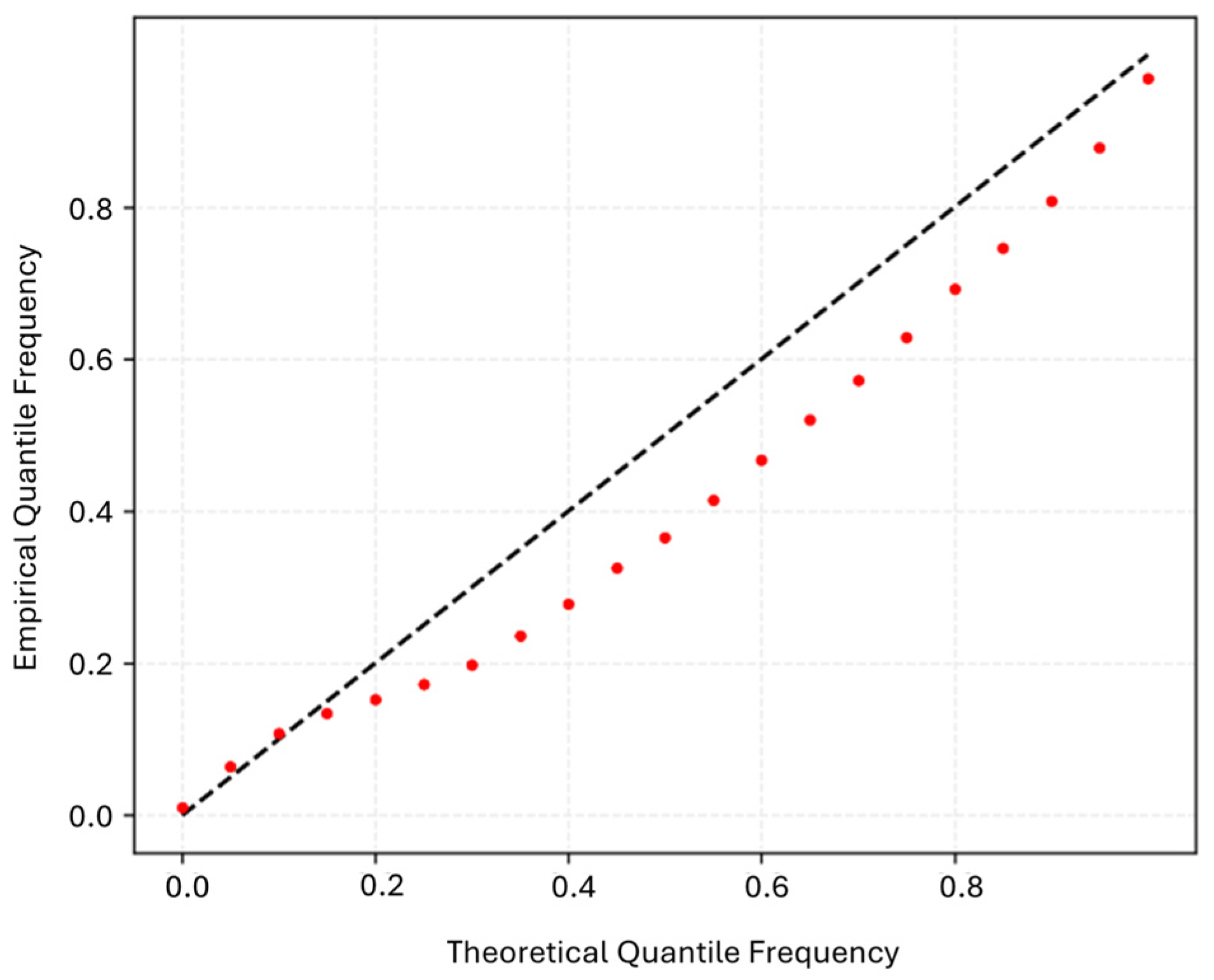
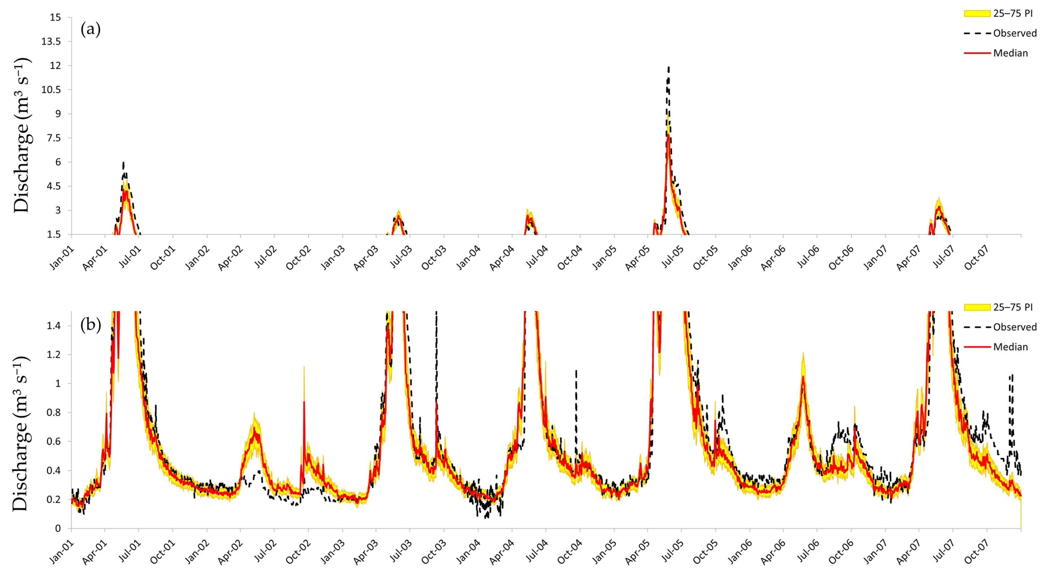
Uncertainty in the model’s streamflow predictions was evaluated using a predictive uncertainty band derived from the GMM regression head. In Figure 3, the x-axis represents the theoretical quantile frequency, while the y-axis shows the relative empirical counts. In Figure 4a,b, the hydrograph shows observed streamflow (dashed line) alongside simulation percentiles for high-flow (>1.5 m3 s−1) conditions (a) and low-flow (<1.5 m3 s−1) conditions (b), with shaded bands denoting the 25–75% predictive interval. Across most of the record, observed discharge falls within or near the central predictive envelope, indicating that the model captures the dominant variability and associated uncertainty under typical hydroclimatic conditions. Deviations outside the interquartile range occur primarily during extreme low- and high-flow periods, reflecting increased predictive uncertainty and systematic bias under hydrologic stress. The overall correspondence between observed and predicted flow, supported by the QQ-plot behavior and validation metrics, indicates that the model performs credibly under typical conditions while still exhibiting limitations during extremes. The next section examines this issue in detail by isolating the drought year, exploring why FLV values are elevated, and evaluating the magnitude mismatch visible in the hydrograph during this extreme period.

Figure 3.
Quantile–Quantile (QQ) Probability Plot Assessing Distributional Agreement Between LSTM-Simulated and Observed Streamflow at the Rio Hondo Gage. Red points represent empirical quantile pairs, and the dashed black line indicates the 1:1 reference line.
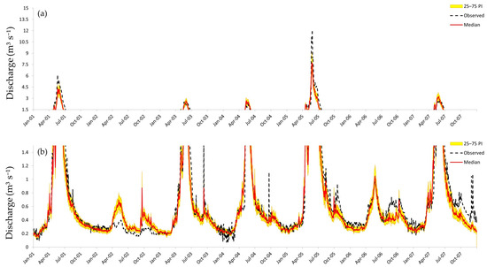
Figure 4.
Predictive uncertainty assessment for the LSTM streamflow model at the Rio Hondo gage. Panels show observed discharge (dashed black), median model prediction (red), and the 25–75% predictive interval (yellow shading) for (a) high-flow conditions (1.5–15 m3 s−1) and (b) low-flow conditions (0–1.5 m3 s−1).
3.3. Baseflow Index Behavior Under Drought and Pre-Drought Conditions
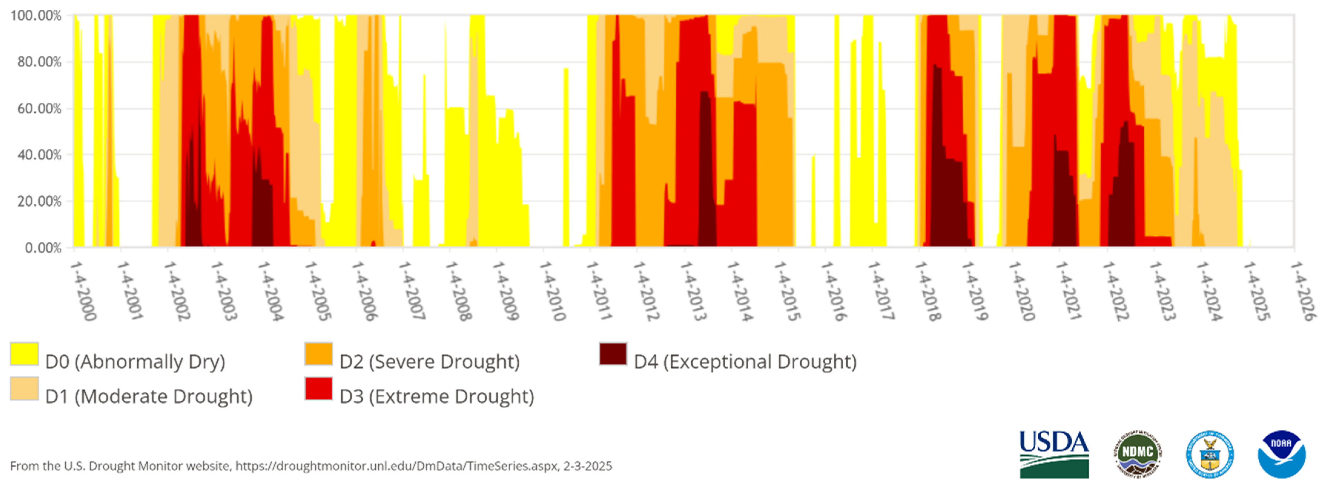
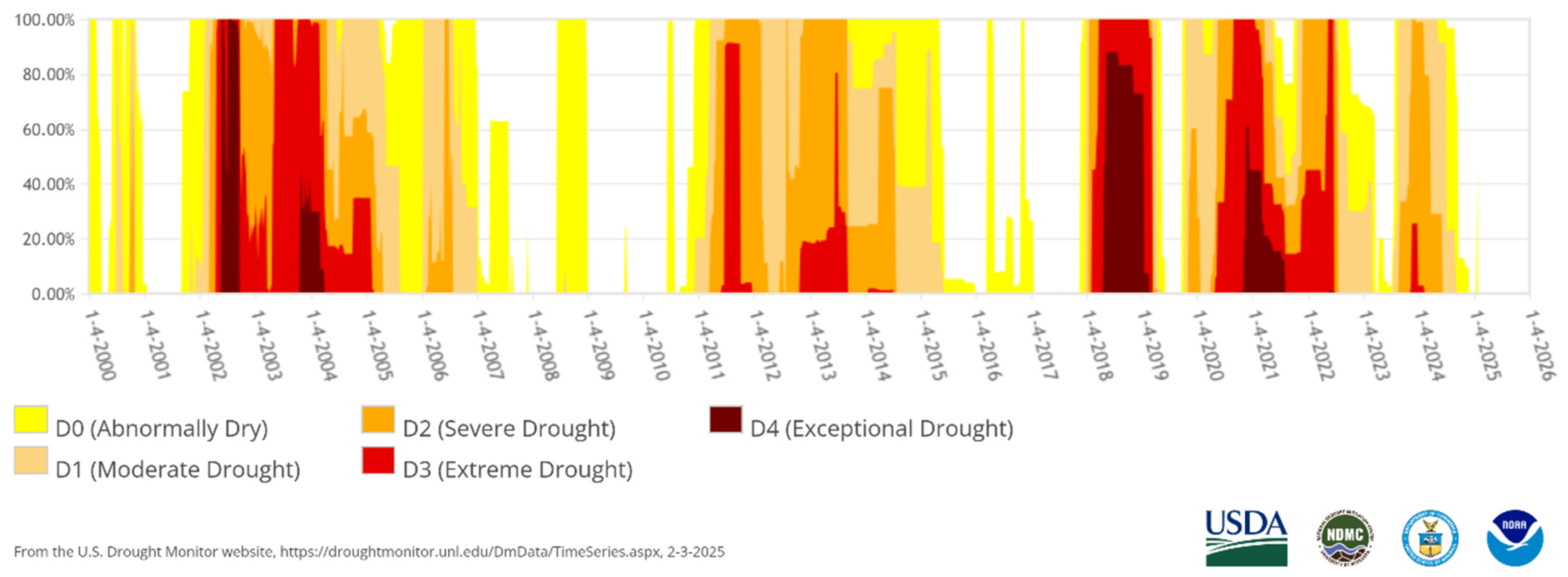
The validation period for this study spanned a period of extended drought from 2002 to 2004. During this period, Taos and Colfax counties, where the study area is located, experienced prolonged Extreme (D3) to Exceptional (D4) drought as classified by the U.S. Drought Monitor (Figure 5 and Figure 6) [72]. The U.S. Drought Monitor is jointly produced by the National Drought Mitigation Center at the University of Nebraska-Lincoln, the United States Department of Agriculture, and the National Oceanic and Atmospheric Administration. Map courtesy of NDMC (National Drought Mitigation Center). Because baseflow behavior in these basins is strongly conditioned by snow accumulation and melt processes, interannual variations in snow fraction and snowpack magnitude were examined to provide hydroclimatic context for the BFI results discussed below.
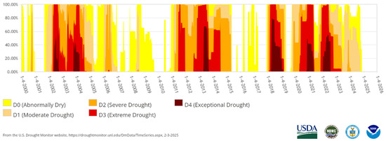
Figure 5.
Percentage of Taos County, New Mexico, within U.S. Drought Monitor categories (D0–D4) from 2000 to 2026. Colors denote drought severity; USDM data (NDMC, USDA, NOAA).
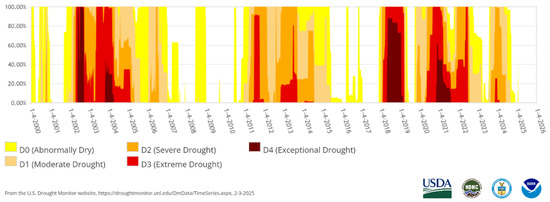
Figure 6.
Percentage of Colfax County, New Mexico, within U.S. Drought Monitor categories (D0–D4) from 2000 to 2026. Colors denote drought severity; USDM data (NDMC, USDA, NOAA).
To provide hydroclimatic context for interpreting baseflow behavior under these conditions, interannual variations in snow fraction and snowpack magnitude derived from the Daymet meteorological dataset used for both LSTM and HEC-HMS model development were examined across pre-drought and drought periods. During pre-drought years (2000–2001), basin-averaged snow fraction values ranged from approximately 42% to 54%, with annual maximum SWE values of approximately 125–130 kg m−2, indicating substantial seasonal snow accumulation. During the subsequent drought period (2002–2004), snow fraction values declined, reaching a minimum of approximately 31% in 2002, and maximum SWE was markedly reduced (≈70 kg m−2 in 2002), reflecting diminished snowpack storage and persistence. For reference, the long-term basin-averaged snow fraction across the full record was approximately 41%, with a mean annual maximum SWE of approximately 150 kg m−2. Although snowfall continued during drought years, reduced snowpack accumulation limited the magnitude and timing of snowmelt-driven runoff, consistent with the muted seasonal variability and persistently low discharge observed in the LSTM hydrographs. This context indicates that streamflow during drought was increasingly governed by delayed groundwater release rather than direct melt-driven runoff.
Table 7 and Table 8 summarize streamflow performance metrics for the LSTM model during pre-drought and drought conditions, respectively, providing quantitative context for interpreting baseflow behavior under contrasting hydroclimatic regimes. Across both periods, the model generally reproduced the timing and relative variability of streamflow, as indicated by high Pearson-r values, while exhibiting larger biases in absolute magnitude during drought years, particularly at low flows as reflected by elevated FLV values. These performance characteristics motivate the use of proportional metrics such as BFI to evaluate changes in hydrologic partitioning independent of discharge magnitude.

Table 7.
Streamflow performance metrics comparing observed and LSTM-simulated daily discharge across the five study basins during pre-drought conditions (2000–2001).

Table 8.
Streamflow performance metrics comparing observed and LSTM-simulated daily discharge across the five study basins during drought conditions (2002–2004).
For this analysis, the BFI, defined as the ratio of mean baseflow to mean total discharge, was computed using the Lyne and Hollick digital filter, to evaluate baseflow representation under drought conditions. BFI was calculated for both pre-drought (2001) and drought (2002–2004) periods using observed and simulated streamflow from the LSTM model. Results show strong agreement between observed and simulated BFI values across most basins and time periods. In pre-drought years, differences were within 0.04 across all basins, with the model slightly overestimating baseflow.
During the drought, both observed and simulated BFI values increased across all basins with the exception of observed Ponil Creek, reflecting the higher proportional contribution of groundwater during dry periods. For Ponil Creek, the simulated BFI (0.29) exceeded the observed (0.21), aligning with earlier observations that the model struggled to adjust to post-fire hydrologic changes.
The FLV and BFI results highlight a critical insight for interpreting subsequent internal-state analyses: although the model exhibited elevated low-flow bias under drought conditions, it still produced BFI values consistent with the observed values. This suggests that the internal LSTM states preserved behavior consistent with the observed hydrologic baseflow partitioning under drought conditions, despite biases in absolute discharge magnitude during extreme low-flow periods. This interpretation is further supported by the Pearson-r values and visual inspection of the hydrograph during this period. High Pearson- values (>0.9), along with well-aligned peaks and recession limbs, indicate good dynamic performance, with the large FLV values reflecting a magnitude bias rather than a structural or temporal error in model behavior. This distinction is important for the next section, which compares the extracted cell states to the decomposed Baseflow-1 and Baseflow-2 signals from HEC-HMS.
How the model responds to drought stress provides additional context for interpreting how baseflow dynamics are represented within the LSTM. During periods of extended drought, baseflow contributions comprise a larger fraction of total streamflow, leading to elevated BFI values. This suggests that the LSTM’s internal memory states responded in a manner consistent with shifts in hydrologic partitioning, even when total discharge declined, as evidenced by reduced mean annual flows during drought years (e.g., mean flow declined from ≈1.02 m3 s−1 in 2001 to ≈0.26 m3 s−1 in 2002 for the Rio Hondo; Table 5) alongside increased observed and simulated BFI values across all basins (Table 9). Rather than responding solely to contemporaneous precipitation inputs, the LSTM’s internal states exhibited behavior consistent with the influence of storage and delayed release processes, allowing the model to preserve the relative contribution of baseflow even when absolute discharge magnitudes were biased. This would suggest that internal-state analysis of LSTM models can provide insight into patterns of groundwater–surface water partitioning reflected in internal model representations under both typical and drought conditions.

Table 9.
Observed and LSTM-simulated Baseflow Index (BFI) during pre-drought (2000–2001) and drought (2002–2004) conditions.
3.4. Evaluating LSTM States Against Simulated Baseflow Components
The BFI digital filter is useful for separating baseflow contributions but does not provide information on subsurface flow paths or groundwater residence times. Mountain groundwater circulation has been shown to include short-term, surface-connected flow paths alongside slow, deep flow paths within fractured bedrock, as conceptually depicted in Figure 7 [73,74]. To further evaluate whether the LSTM internally represented baseflow-related dynamics, activations of the LSTM cell state and hidden state units were extracted, and regression analyses were performed between individual LSTM units and baseflow estimates derived from the physically based HEC-HMS model outlined in Section 2.2 for the Rio Hondo basin.
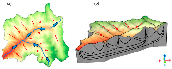
Figure 7.
Conceptual schematic of streamflow generation in high-elevation mountain basins, adapted for the Rio Hondo basin from [74], illustrating (a) hillslope runoff and shallow subsurface flow and (b) delayed groundwater discharge from high-elevation recharge through long subsurface flow paths. Blue arrows denote main channels, red arrows indicate surface runoff, and black arrows represent groundwater circulation. Three-dimensional orientation is depicted in the bottom right.
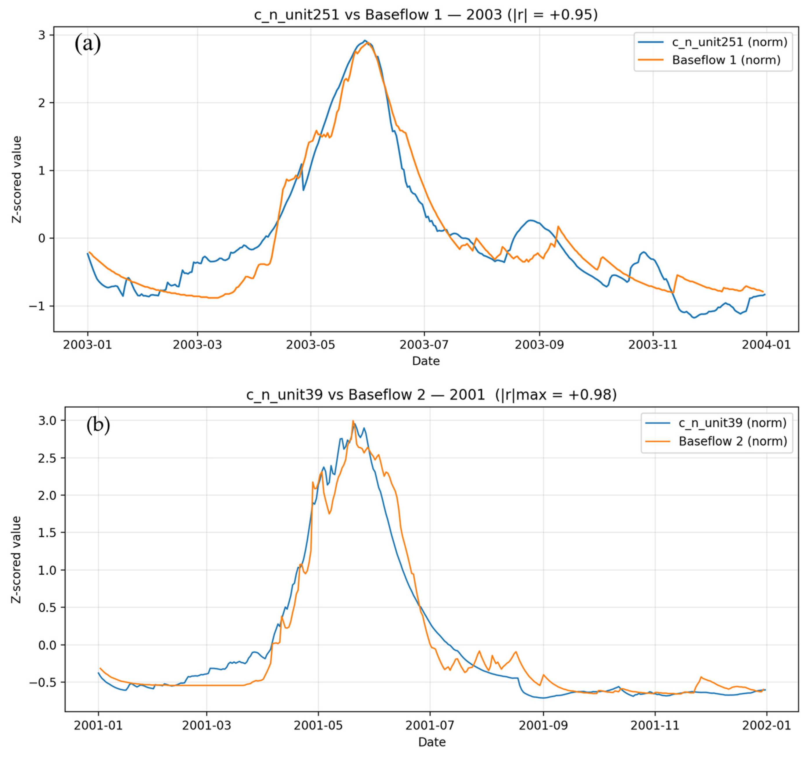
In the HEC-HMS framework, GW-1 represents a fast-responding, shallow groundwater reservoir associated with near-surface storage and hillslope drainage, while GW-2 represents a slower-responding, deeper groundwater reservoir associated with delayed discharge from fractured bedrock and deeper subsurface storage [75]. The correlation analysis revealed multiple internal memory units with high (>0.85) absolute correlation. Figure 8 illustrates examples of patterns and relationships between extracted memory states and baseflow components. The traces labeled c_n_unit_XXX correspond to the internal LSTM cell states of individual units within the 256-unit core, plotted here to highlight their alignment with hydrologic baseflow dynamics. These results suggest that the LSTM’s internal states captured patterns statistically consistent with subsurface hydrologic dynamics. Specifically, it developed internal representations consistent with both groundwater discharge and storage behavior.
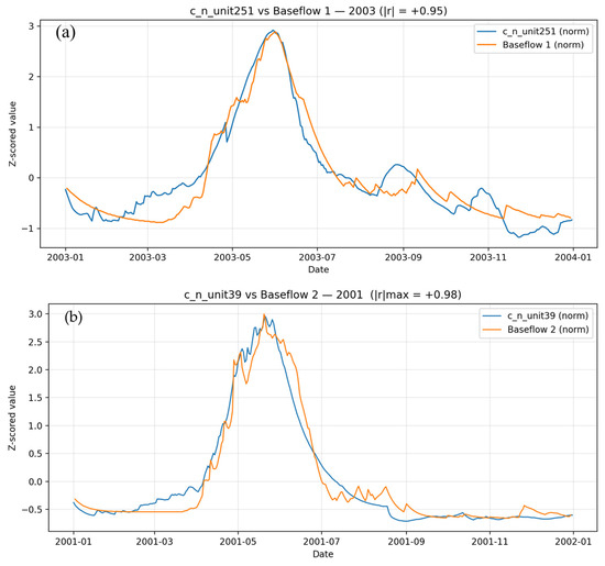
Figure 8.
Normalized LSTM cell state activations plotted against normalized HEC-HMS baseflow components, showing (a) strong positive correlation with Baseflow-1, representing fast-responding shallow groundwater and near-surface storage, and (b) strong positive correlation with Baseflow-2, representing slower-responding deep groundwater and delayed subsurface discharge.
It is important to note that while baseflow is measured in cubic meters per second, the LSTM cell state activations are unitless. For ease of visualization in Figure 8, these values have been normalized using Z-score transformation to rescale each dataset to have a mean of 0 and standard deviation of 1. Additionally, the peaks in the activation patterns do not align perfectly with the baseflow estimates. This misalignment may arise from several factors. First, the internal representations of machine learning models like LSTMs are inherently opaque, and how the model stores or interprets hydrological information cannot be directly observed. Second, discrepancies may stem from limitations in the HEC-HMS model, such as imperfect calibration or structural assumptions. Third, the HEC-HMS model computes baseflow at a fixed outlet location, whereas the LSTM may associate groundwater influence with different spatial or temporal reference points. In particular, the LSTM internal states may represent groundwater influence as a basin-integrated or temporally lagged storage signal rather than as an instantaneous baseflow flux at the outlet, leading to systematic phase offsets when compared to outlet-based conceptual baseflow estimates.
4. Discussion
4.1. Correlation with Evolved Groundwater Study
To assess the physical relevance of the LSTM’s internal memory states in a subsurface-dominated setting, internal-state behavior was examined against an independent, physically grounded hydrochemical benchmark. The EMMA comparison is intentionally limited in scope and is not intended as a quantitative validation of model predictions. Instead, it provides qualitative physical context from an independent hydrochemical perspective, evaluates whether internal LSTM states align with established groundwater residence-time classifications, and serves as a hypothesis-generating tool for exploring how subsurface flow-path and storage-related timescales may be reflected in the organization of the model’s internal memory states. Given the limited number of discrete EMMA sampling dates, the analysis emphasizes structural consistency and directional agreement rather than statistical inference.
Consistent with this interpretive framework, LSTM state activations were extracted and compared to groundwater source contributions estimated from a prior EMMA study in the Rio Hondo basin [35]. That study used isotopic and geochemical tracers (e.g., δ18O, δ2H, Ca2+, Mg2+, Na+, SiO2) to classify streamflow into three source categories: evolved groundwater, moderately evolved water, and very immature water. Very immature water represents short residence-time flow paths associated with rapid hydrologic response (e.g., recent snowmelt or shallow subsurface flow), whereas evolved groundwater reflects long residence times and deeper subsurface circulation that sustain baseflow during late-season and drought conditions; moderately evolved water represents intermediate storage and flow-path lengths between these end members. Contributions from each source were estimated for 11 discrete sampling dates between March 2012 and March 2013 using Principal Component Analysis (PCA) defined mixing subspaces [76]. Only tracers with well-behaved residuals (p > 0.05, R2 < 0.4) were used, ensuring physical interpretability.
For each EMMA sampling date, internal state information was extracted from the LSTM model for the corresponding date, and Pearson correlations were computed between individual LSTM units and the fractional contribution of each groundwater class. It is important to note that the LSTM’s internal memory states and the EMMA-derived groundwater fractions do not share identical temporal or spatial reference points. EMMA estimates represent outlet-integrated source-water contributions at discrete sampling dates, whereas LSTM states reflect temporally integrated representations of antecedent hydrologic conditions learned from continuous forcing data. As a result, observed correlations do not imply one-to-one correspondence but instead indicate that LSTM internal memory states capture groundwater-related signals with different temporal reference frames that remain consistent with the underlying flow path and residence-time structure inferred from EMMA. The top ten correlations for each groundwater source were plotted and can be seen in Figure 9.
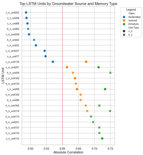
Figure 9.
Absolute Pearson correlations between selected LSTM’s memory units and EMMA-derived groundwater source fractions. Colors represent groundwater source class, marker shape indicates memory type (cn vs. hn), and the red line denotes the statistical significance threshold (|r| = 0.60, n = 11).
To determine whether these correlations were significant a t-test was performed for the Pearson correlation coefficient. Using a sample size of 11 and a significance level of 0.05 it was determined that a Pearson r > 0.60 was taken to be significant. Using this metric and the information from Figure 9, it can be seen that the highest correlation was for the immature groundwater, followed by evolved, then moderately evolved, with only evolved and immature groundwater demonstrating significant correlation.
This suggests that the LSTM’s internal states exhibited stronger and more consistent alignment with immature and evolved groundwater signatures, while correspondence with moderately evolved groundwater sources was weaker. To determine whether these high-correlation units shared common response patterns across all groundwater classes, and whether such patterns reflected underlying hydrologic processes, the full correlation profiles of each unit were then examined using clustering and PCA. Importantly, no groundwater source influence ratios or weighting criteria were prescribed in the clustering analysis. Each LSTM unit was represented by a three-element vector consisting of its Pearson correlation coefficients with the evolved, moderately evolved, and immature groundwater fractions derived from the EMMA study. Prior to clustering, these correlation vectors were standardized to zero mean and unit variance across groundwater classes to ensure equal scaling and to prevent any single source from disproportionately influencing the distance metric. Clustering was then performed directly in this standardized correlation space, such that units were grouped solely based on similarity in their overall correlation patterns rather than the dominance of any individual groundwater contribution.
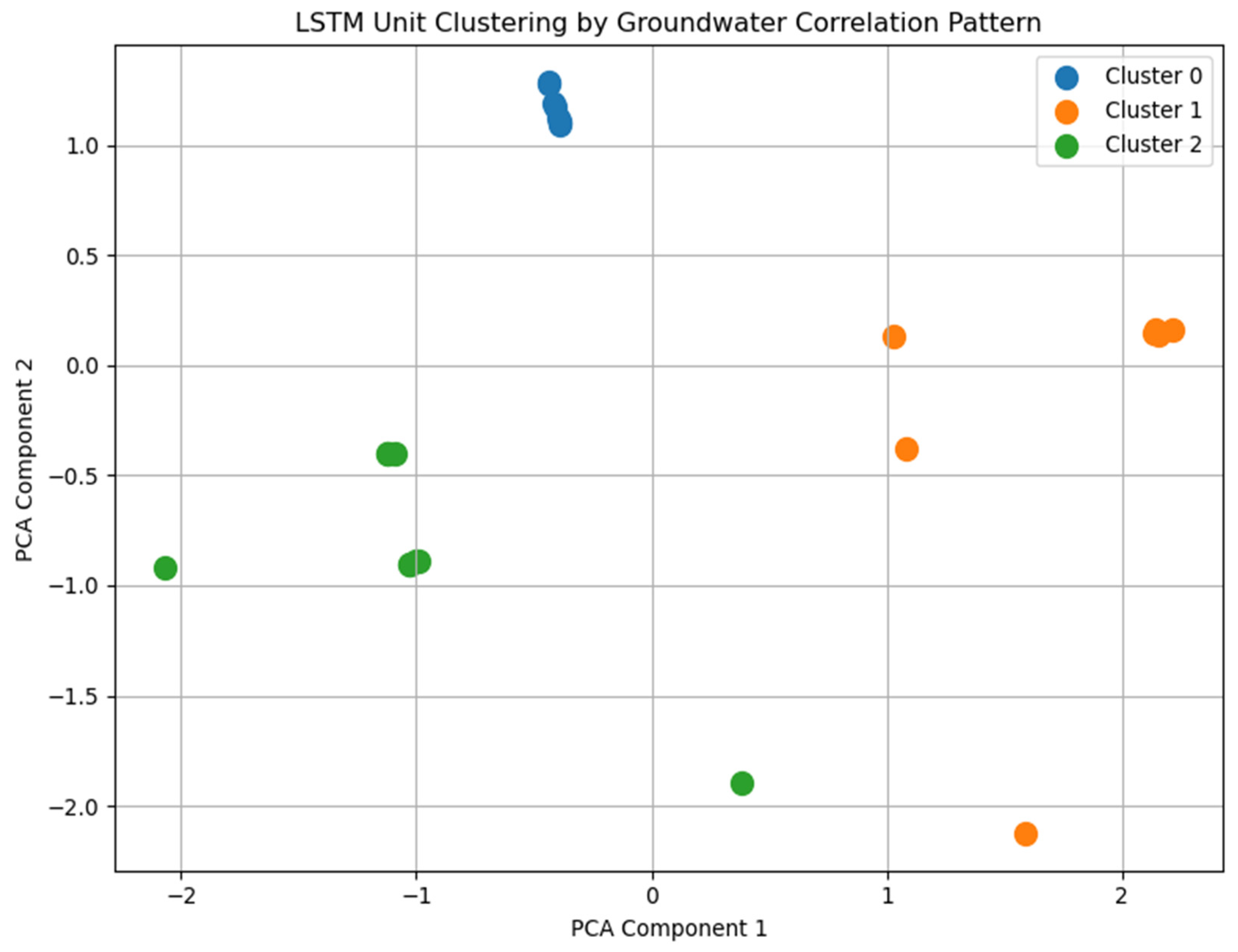
Although alternative cluster numbers are geometrically plausible in the reduced correlation space, three clusters were specified to provide an interpretable comparison with the three EMMA-derived groundwater residence-time classes; importantly, the interpretation relies on the structure and continuity of correlation patterns rather than the exact number of clusters, such that increasing or decreasing k would refine granularity without altering the underlying conclusions. When clustered into three groups, LSTM units exhibited distinct patterns of association with the EMMA-derived groundwater fractions (Figure 10). These groups were characterized by differences in their correlation profiles across evolved, moderately evolved, and immature groundwater sources, providing a structured basis for comparing internal memory behavior across groundwater residence-time regimes. When visualized using PCA, the clustered units also exhibited non-random composition with respect to memory type (hn vs. cn), suggesting that groundwater-related correlation patterns were associated with differences in temporal memory characteristics. This convergence between internal model organization and physically meaningful hydrologic distinctions is encouraging, although the limited sample size of 11 discrete EMMA sampling dates constrains statistical power. With such sparse temporal coverage, the analysis may overlook subtler or transient relationships between groundwater contributions and internal states. Future studies incorporating higher-frequency isotope and geochemical sampling would enable more rigorous evaluation of these patterns and finer discrimination of how source-water signatures are reflected in model memory. With more temporally resolved hydrochemical data, increasing the number of clusters could enable identification of finer-scale groundwater sub-regimes within the broader evolved, moderately evolved, and immature classes, potentially revealing multiple storage and flow-path timescales encoded within the model’s internal memory states.

Figure 10.
PCA visualization of clustered LSTM units based on standardized correlation patterns with EMMA-derived groundwater source fractions. Colors indicate unsupervised cluster membership, highlighting distinct groundwater-association regimes among memory units.
4.2. Implications for Interpretability and Water Management
In northern New Mexico, headwater streams originating in the Sangre de Cristo Mountains provide essential water supplies to small rural communities through a combination of surface-water diversions and shallow alluvial groundwater use. Sustained baseflow is particularly important during prolonged dry periods, when snowmelt contributions are reduced and groundwater discharge becomes the dominant source of streamflow. In such settings, shifts in groundwater contribution influence seasonal water availability and drought vulnerability. Beyond predictive accuracy alone, the ability of the LSTM to internally distinguish between fast runoff and delayed groundwater contributions suggests that internal-state diagnostics may offer a complementary, process-oriented means of evaluating groundwater dependence and hydrologic resilience in snowmelt-dominated, semi-arid basins where direct groundwater observations are sparse. While such applications would require careful validation and should not be viewed as a substitute for physical measurements or regulatory analysis, these results highlight a potential role for data-driven models in supporting decision-relevant assessments of groundwater–surface water interactions under hydroclimatic stress.
4.3. Wildfire Disturbances
Upon inspecting the validation metrics, Ponil Creek showed the lowest performance across all metrics. One explanation for this would be the Ponil Complex Fires. These were a series of lightning-caused wildfires in New Mexico that burned a total of 92,470 acres and the majority of the Ponil Creek watershed [77]. The observed data followed the expected post wildfire trends with large spikes corresponding with precipitation events [78,79]. In contrast, the predicted values continued to follow the pre-disturbance seasonal patterns learned during training and failed to capture these post-fire responses.
As the machine learning model employed static basin attributes and lacked disturbance-sensitive inputs, it had no mechanism to adapt to rapid changes in land use, land cover, or surface hydrologic processes following wildfire. This limitation underscores an important direction for future hydrologic model development, particularly in disturbance-prone regions. Potential improvements include incorporating dynamic attributes such as burn severity or burn area indices to represent disturbance onset, alongside remotely sensed indicators such as the Normalized Difference Vegetation Index (NDVI) and surface temperature to capture vegetation recovery and evolving surface energy conditions.
From a management perspective, the wildfire case highlights a key limitation of current data-driven hydrologic models when applied in disturbance-prone regions. Post-fire increases in runoff magnitude and altered flow timing have direct implications for flood risk, sediment transport, and water quality, yet these effects are not captured unless disturbance-sensitive information is incorporated. The results underscore the importance of integrating dynamic land-surface indicators—such as burn severity, vegetation recovery, or soil hydrophobicity—into both predictive and interpretive hydrologic models to support post-disturbance water management and hazard mitigation.
4.4. Context and Limitations
Several limitations should be noted when interpreting these results. First, the internal-state analysis relied on decomposed GW-1 and GW-2 signals from HEC-HMS, which serve as physically informed proxies for shallow and deep baseflow rather than direct measurements of groundwater discharge. While this approach provides a useful comparative framework, it inherits the structural assumptions and parameter sensitivities of the HEC-HMS model itself. In addition, the analysis did not incorporate continuous in situ groundwater level measurements or basin-interior meteorological observations, relying instead on gridded forcing products and conceptual representations due to data availability constraints. Second, the LSTM exhibited systematic low-flow magnitude biases, particularly during drought years, as reflected by elevated FLV values. Although the model reproduced recession timing and baseflow partitioning reasonably well, these magnitude errors indicate that its representation of hydrologic memory is not without limitations. Third, the isotopic end-member comparison offered only preliminary insight due to sparse temporal coverage, limiting the ability to directly validate residence-time interpretations. Taken together, these factors highlight that the inferred correspondence between LSTM states and hydrologic processes, while compelling, should be viewed as provisional pending further validation with higher-resolution discharge, groundwater, and tracer datasets. Fourth, it should be emphasized that internal LSTM’s memory states are not interpreted as direct simulations or measurements of groundwater fluxes or storage but rather as latent representations whose temporal behavior can be compared to physically derived benchmarks to assess process consistency. Fifth, the analysis was conducted on a limited number of relatively small, snowmelt-dominated headwater basins. While this focus enabled detailed process-oriented interpretation, it may limit the direct extrapolation of findings to larger, more heterogeneous watersheds or systems with substantial human regulation, complex stratigraphy, or multiple interacting aquifer units. Lastly, although this study did not employ formal XAI techniques, permutation importance, or attention mechanisms, the results highlight how internal-state analysis can serve as a complementary interpretability framework for recurrent hydrologic models. XAI methods are well suited for diagnosing input relevance and nonlinear sensitivities, whereas internal-state approaches emphasize how information is stored, integrated, and released over time within the model. Future work could integrate these perspectives by combining state-based diagnostics with attribution-based XAI, enabling a more complete interpretation of both the drivers and internal mechanisms governing model behavior under varying hydroclimatic conditions.
5. Conclusions
This study examined whether LSTM models trained solely on meteorological and hydrologic inputs can internally encode information consistent with groundwater-driven baseflow dynamics in snowmelt-dominated, semi-arid mountain basins. Using five headwater catchments in northern New Mexico, LSTM’s internal memory states were evaluated against physically informed baseflow proxies derived from a conceptual HEC-HMS model, digital baseflow separation, and independent hydrochemical context.
The results show that LSTM’s cell state units developed statistically and conceptually consistent patterns associated with baseflow behavior. Distinct subsets of memory states aligned preferentially with fast and slow groundwater response components, consistent with shallow and deep subsurface flow paths, and these internal representations remained coherent under contrasting hydroclimatic conditions, including prolonged drought. These findings indicate that LSTM’s internal states can capture temporally persistent groundwater-related signals without explicit baseflow targets during training.
Comparison with a previously published end-member mixing analysis provided qualitative, physically grounded context, suggesting correspondence between LSTM’s memory patterns and groundwater source classes associated with differing residence times. Although limited by sparse temporal resolution, this comparison supports the interpretation that internal-state analysis can reveal emergent hydrologic structure rather than purely statistical associations.
Several limitations should be noted. Baseflow estimates were derived from conceptual models and digital filters rather than direct groundwater measurements, and hydrochemical observations were temporally sparse, limiting the ability to formally validate inferred residence-time relationships. In addition, model performance exhibited low-flow magnitude biases during drought periods, and the analysis was conducted on a limited number of small, snowmelt-dominated headwater basins, which may constrain broader generalization. Accordingly, the relationships identified between LSTM internal memory states and groundwater-related processes should be viewed as indicative rather than definitive, motivating future work using higher-resolution discharge, groundwater, and tracer observations.
Despite these limitations, this study demonstrates that interrogating internal LSTM states offers a complementary interpretability pathway to attribution-based explainable artificial intelligence methods by emphasizing how hydrologic information is stored, integrated, and released over time within recurrent models. By linking internal memory behavior to independently derived baseflow estimates and groundwater residence-time indicators, the results illustrate how data-driven models can encode physically meaningful process information beyond predictive performance alone. Future work should prioritize higher-frequency groundwater and hydrochemical observations, expansion to additional hydroclimatic regions, and integration of disturbance-sensitive processes to further evaluate the robustness and generality of these findings.
Author Contributions
M.R.: writing—original draft, editing, visualization, methodology, formal analysis, data curation, conceptualization, software; Y.H.L.: conceptualization, methodology, project administration, supervision; K.Z.: conceptualization, methodology, project administration, supervision; K.S.: review, editing. All authors have read and agreed to the published version of the manuscript.
Funding
This research received no external funding.
Data Availability Statement
The data presented in this study are derived from publicly accessible repositories. Daily meteorological forcing data were obtained from the Daymet Daily Surface Weather Data product distributed by the Oak Ridge National Laboratory Distributed Active Archive Center (ORNL DAAC) (DOI: https://doi.org/10.3334/ORNLDAAC/2129), accessed via the NASA AppEEARS data access service. Historical water balance variables were obtained from the National Park Service Historical Water Balance, Daily dataset, documented in the associated peer-reviewed data description (DOI: https://doi.org/10.1002/ecs2.4530) and accessed via NASA AppEEARS. Basin characteristics and streamflow data were obtained from the U.S. Geological Survey StreamStats database (DOI: https://doi.org/10.5066/F7T72FXQ) and the U.S. Geological Survey National Water Information System (NWIS) (https://waterdata.usgs.gov (accessed on 16 June 2020)). Hydrochemical context data used for qualitative comparison were obtained from a publicly available Master’s thesis [35], with relevant data provided in the appendices of the thesis (https://www.nmt.edu/academics/ees/theses/theses_1936-2014/2014t_tolley%20iii_dg.pdf (accessed on 6 June 2025)). Model training and evaluation were performed using the open-source NeuralHydrology framework (https://github.com/neuralhydrology/neuralhydrology (accessed on 12 December 2024)). All data sources are publicly available and were accessed as described above.
Conflicts of Interest
The authors declare no conflicts of interest.
Abbreviations
The following abbreviations are used in this manuscript:
| LSTM | Long Short-Term Memory |
| XAI | Explainable Artificial Intelligence |
| HEC-HMS | Hydrologic Engineering Center’s Hydrologic Modeling System |
| EMMA | End-Member Mixing Analysis |
| GMM | Gaussian Mixture Model |
| NPS | National Parks Service |
| DHWBDP | Daily Historical Water Balance Data Product |
| SWE | Snow Water Equivalent |
| USGS | United States Geological Survey |
| BFI | Baseflow Index |
| NLCD | National Land Cover Database |
| SSURGO | Soil Survey Geographic Database |
| NSE | Nash-Sutcliffe Efficiency |
| ATI | Antecedent Temperature Index |
| RMSE | Root Mean Square Error |
| NRMSE | Normalized Root Mean Square Error |
| PBIAS | Percent Bias |
| R2 | Coefficient of Determination |
| KGE | Kling-Gupta Efficiency |
| FMS | Medium flow bias |
| FLV | Low flow bias |
| FDC | Flow Duration Curve |
| Quantile-Quantile | |
| NDMC | National Drought Mitigation Center |
| PCA | Principle Component Analysis |
| NDVI | Normalized Difference Vegetation Index |
References
- Carroll, R.; Manning, A.H.; Niswonger, R.G.; Marchetti, D.W.; Williams, K.H. Baseflow age distributions and depth of active groundwater flow in a snow-dominated mountain headwater basin. Water Resour. Res. 2020, 56, e2020WR028161. [Google Scholar] [CrossRef]
- Godsey, S.E.; Kirchner, J.W.; Tague, C. Effects of changes in winter snowpacks on summer low flows: Case studies in the Sierra Nevada, California, USA. Hydrol. Process. 2013, 28, 5048–5064. [Google Scholar] [CrossRef]
- Schilling, O.S.; Parajuli, A.; Otis, C.T.; Müller, T.; Quijano, W.A.; Tremblay, Y.; Therrien, R. Quantifying groundwater recharge dynamics and unsaturated zone processes in snow-dominated catchments via on-site dissolved gas analysis. Water Resour. Res. 2021, 57, e2020WR028479. [Google Scholar] [CrossRef]
- Tennant, C.; Larsen, L.G.; Bellugi, D.; Moges, E.; Zhang, L.; Ma, H. The utility of information flow in formulating discharge forecast models: A case study from an arid snow-dominated catchment. Water Resour. Res. 2020, 56, e2019WR024908. [Google Scholar] [CrossRef]
- Huntington, J.; Niswonger, R.G. Role of surface-water and groundwater interactions on projected summertime streamflow in snow-dominated regions: An integrated modeling approach. Water Resour. Res. 2012, 48, W11503. [Google Scholar] [CrossRef]
- Frisbee, M.D.; Tolley, D.G.; Wilson, J.L. Field estimates of groundwater circulation depths in two mountainous watersheds in the western US and the effect of deep circulation on solute concentrations in streamflow. Water Resour. Res. 2017, 53, 2693–2715. [Google Scholar] [CrossRef]
- Brooks, P.D.; Solomon, D.K.; Kampf, S.; Warix, S.; Bern, C.; Barnard, D.; Barnard, H.R.; Carling, G.T.; Carroll, R.W.H.; Chorover, J.; et al. Groundwater dominates snowmelt runoff and controls streamflow efficiency in the western United States. Commun. Earth Environ. 2025, 6, 341. [Google Scholar] [CrossRef]
- Frisbee, M.D.; Phillips, F.M.; White, A.F.; Campbell, A.R.; Liu, F. Effect of source integration on the geochemical fluxes from springs. Appl. Geochem. 2013, 28, 32–54. [Google Scholar] [CrossRef]
- Ajami, H.; Troch, P.A.; Maddock, T. Quantifying mountain block recharge by means of catchment-scale storage–discharge relationships. Water Resour. Res. 2011, 47, W04507. [Google Scholar] [CrossRef]
- Ciruzzi, D.M.; Lowry, C.S. Impact of complex aquifer geometry on groundwater storage in high-elevation meadows of the Sierra Nevada Mountains, California. Hydrol. Process. 2017, 31, 1565–1579. [Google Scholar] [CrossRef]
- Werth, S.; Shirzaei, M.; Carlson, G.; Bürgmann, R. Connecting Deep Aquifer Recharge in California’s Central Valley to Sierra Nevada Snowmelt via Multi-Sensor Remote Sensing Data. EGUsphere 2025, 2025, 1–35. [Google Scholar]
- Fan, L.; Kuang, X.; Or, D.; Zheng, C. Streamflow Composition and Water “Imbalance” in the Northern Himalayas. Water Resour. Res. 2023, 59, e2022WR034243. [Google Scholar] [CrossRef]
- Luce, C.H.; Holden, Z.A. Declining annual streamflow distributions in the Pacific Northwest United States, 1948–2006. Geophys. Res. Lett. 2009, 36, L16401. [Google Scholar] [CrossRef]
- Manning, A.H.; Solomon, D.K. An integrated environmental tracer approach to characterizing groundwater circulation in a mountain block. Water Resour. Res. 2005, 41, W12403. [Google Scholar] [CrossRef]
- Liu, B.; Tang, Q.; Zhao, G.; Gao, L.; Shen, C.; Pan, B. Physics-Guided Long Short-Term Memory Network for Streamflow and Flood Simulations in the Lancang–Mekong River Basin. Water 2022, 14, 1429. [Google Scholar] [CrossRef]
- Yu, H.; Yang, Q. Applying Machine Learning Methods to Improve Rainfall–Runoff Modeling in Subtropical River Basins. Water 2024, 16, 2199. [Google Scholar] [CrossRef]
- Yu, Q.; Chen, X.; Du, Y.; Liu, Y.; Li, Q.; Ma, Y. Enhancing long short-term memory (LSTM)-based streamflow prediction with a spatially distributed approach. Hydrol. Earth Syst. Sci. 2024, 28, 2107–2122. [Google Scholar] [CrossRef]
- Hunt, K.M.R.; Brown, J.D.; Jones, S.A.; Liu, Z. Using a long short-term memory (LSTM) neural network to boost river streamflow forecasts over the western United States. Hydrol. Earth Syst. Sci. 2022, 26, 5449–5472. [Google Scholar] [CrossRef]
- Kratzert, F.; Klotz, D.; Herrnegger, M.; Sampson, A.K.; Hochreiter, S.; Nearing, G.S. Rainfall–runoff modelling using long short-term memory (LSTM) networks. Hydrol. Earth Syst. Sci. 2018, 22, 6005–6022. [Google Scholar] [CrossRef]
- Solanki, H.; Vegad, U.; Kushwaha, A.P.; Mishra, V. Improving streamflow prediction using multiple hydrological models and machine learning methods. Water Resour. Res. 2025, 61, e2024WR038192. [Google Scholar] [CrossRef]
- Yifru, B.A.; Lim, K.J.; Lee, S. Enhancing streamflow prediction physically consistently using process-based modeling and domain knowledge: A review. Sustainability 2024, 16, 1376. [Google Scholar] [CrossRef]
- Lees, T.; Chaney, N.; Nearing, G.S.; Xu, Y.; Klotz, D.; Kratzert, F. Hydrological concept formation inside long short-term memory (LSTM) networks. Hydrol. Earth Syst. Sci. Discuss. 2021, 26, 3079–3101. [Google Scholar] [CrossRef]
- Feng, D.; Fang, K.; Shen, C. Enhancing streamflow forecast and extracting insights using long short-term memory networks with data integration at continental scales. Water Resour. Res. 2020, 56, e2019WR026793. [Google Scholar] [CrossRef]
- Hu, C.; Wu, Q.; Li, H.; Jian, S.; Li, N.; Lou, Z. Deep learning with a long short-term memory networks approach for rainfall–runoff simulation. Water 2018, 10, 1543. [Google Scholar] [CrossRef]
- Kratzert, F.; Klotz, D.; Shalev, G.; Klambauer, G.; Hochreiter, S.; Nearing, G. Towards learning universal, regional, and local hydrological behaviors via machine learning applied to large-sample datasets. Hydrol. Earth Syst. Sci. 2019, 23, 5089–5110. [Google Scholar] [CrossRef]
- Mangukiya, N.K.; Sharma, A. Deep learning-based approach for enhancing streamflow prediction in watersheds with aggregated and intermittent observations. Water Resour. Res. 2024, 61, e2024WR037331. [Google Scholar] [CrossRef]
- Anderson, S.; Radić, V. Interpreting deep machine learning for streamflow modeling across glacial, nival, and pluvial regimes in southwestern Canada. Front. Water 2022, 4, 934709. [Google Scholar] [CrossRef]
- Núñez, J.; Cortés, C.B.; Yáñez, M.A. Explainable artificial intelligence in hydrology: Interpreting black-box snowmelt-driven streamflow predictions in an arid Andean basin of north-central Chile. Water 2023, 15, 3369. [Google Scholar] [CrossRef]
- Shrestha, S.G.; Pradhanang, S.M. Performance of LSTM over SWAT in rainfall–runoff modeling in a small, forested watershed: A case study of Cork Brook, RI. Water 2023, 15, 4194. [Google Scholar] [CrossRef]
- Kraft, B.; Jung, M.; Körner, M.; Koirala, S.; Reichstein, M. Towards hybrid modeling of the global hydrological cycle. Hydrol. Earth Syst. Sci. 2022, 26, 1579–1614. [Google Scholar] [CrossRef]
- Joshi, D.C.; Kayastha, R.B.; Shrestha, K.L.; Kayastha, R.B. A hybrid approach to enhance streamflow simulation in data-constrained Himalayan basins: Combining the glacio-hydrological degree-day model and recurrent neural networks. Proc. IAHS 2024, 387, 17–24. [Google Scholar] [CrossRef]
- Bales, R.C.; Molotch, N.P.; Painter, T.H.; Dettinger, M.D.; Rice, R.; Dozier, J. Mountain hydrology of the western United States. Water Resour. Res. 2006, 42, W08432. [Google Scholar] [CrossRef]
- Manning, A.H.; Solomon, D.K.; Sheldon, A.L. Applications of a total dissolved gas pressure probe in ground water studies. Groundwater 2003, 41, 440–448. [Google Scholar] [CrossRef] [PubMed]
- Smerdon, B.D.; Gardner, W.P.; Harrington, G.A.; Tickell, S.J. Identifying the contribution of regional groundwater to the baseflow of a tropical river (Daly River, Australia). J. Hydrol. 2012, 464–465, 107–115. [Google Scholar] [CrossRef]
- Tolley, D.G. High-Elevation Mountain Streamflow Generation: The Role of Deep Groundwater in the Rio Hondo Watershed, Northern New Mexico. Ph.D. Thesis, New Mexico Institute of Mining and Technology, Socorro, NM, USA, 2014. [Google Scholar]
- Huijgevoort, M.v.; Hazenberg, P.; Lanen, H.v.; Uijlenhoet, R. A generic method for hydrological drought identification across different climate regions. Hydrol. Earth Syst. Sci. 2012, 16, 2437–2451. [Google Scholar] [CrossRef]
- Wigington, P.J.; Leibowitz, S.G.; Comeleo, R.L.; Ebersole, J.L. Oregon hydrologic landscapes: A classification framework. J. Am. Water Resour. Assoc. 2012, 49, 163–182. [Google Scholar] [CrossRef]
- U.S. Geological Survey (USGS). Groundwater in the Cimarron River Basin, New Mexico, Colorado, Kansas, and Oklahoma; U.S. Geological Survey: Washington, DC, USA, 1966; Open-File Report 66–159; p. 51. Available online: https://pubs.usgs.gov/publication/ofr66159 (accessed on 16 June 2020).
- Spiegel, Z.; Baldwin, B. Geology and Water Resources of the Santa Fe Area, New Mexico; Geological Survey Water-Supply Paper 1525; U.S. Government Printing Office: Washington, DC, USA, 1963.
- Bauer, P.W.; Johnson, P.S.; Kelson, K.I. Geology and Hydrogeology of the Southern Taos Valley, Taos County, New Mexico; Final Technical Report; New Mexico Office of the State Engineer: Santa Fe, NM, USA, 1999; p. 56.
- Smith, J.F., Jr.; Ray, L.L. Geology of the Cimarron Range, New Mexico. Geol. Soc. Am. Bull. 1943, 54, 891–924. [Google Scholar] [CrossRef]
- Goodknight, C.S. Cenozoic structural geology of the central Cimarron Range, New Mexico. In Guidebook of the 27th Field Conference, New Mexico Geological Society; New Mexico Geological Society: Socorro, NM, USA, 1976; Volume 27, pp. 137–140. [Google Scholar]
- Kratzert, F.; Hochreiter, S.; Klotz, D.; Brandstetter, J.; Mayr, A.; Klambauer, G. NeuralHydrology—A Python library for deep learning research in hydrology. J. Open Source Softw. 2022, 7, 4050. [Google Scholar] [CrossRef]
- NeuralHydrology. GMM—NeuralHydrology Documentation. Available online: https://neuralhydrology.readthedocs.io/en/latest/usage/models.html#gmm (accessed on 15 September 2025).
- Ha, D. Mixture Density Networks with Tensorflow. Available online: http://blog.otoro.net/2015/11/24/mixture-density-networks-with-tensorflow (accessed on 15 September 2025).
- PyTorch. AdamW—PyTorch 2.8 Documentation. Available online: https://pytorch.org/docs/stable/generated/torch.optim.AdamW.html (accessed on 15 September 2025).
- NeuralHydrology. GMM Loss—NeuralHydrology Documentation. Available online: https://neuralhydrology.readthedocs.io/en/latest/api/neuralhydrology.training.loss.html#module-neuralhydrology.training.loss (accessed on 15 September 2025).
- Li, Q.; Zhao, T. Role of the Water Balance Constraint in the Long Short-Term Memory Network: Large-Sample Tests of Rainfall–Runoff Prediction. EGUsphere 2024, 2024, 1–25. [Google Scholar] [CrossRef]
- Mena, J.B.R.; Plaza, D.; Giraldo, E. Multivariate hydrological modelling based on long short-term memory networks for water level forecasting. Information 2024, 15, 358. [Google Scholar] [CrossRef]
- Hu, R.; Fang, F.; Pain, C.C.; Navon, I.M. Rapid spatio-temporal flood prediction and uncertainty quantification using a deep learning method. J. Hydrol. 2019, 575, 911–920. [Google Scholar] [CrossRef]
- Karpatne, A.; Atluri, G.; Faghmous, J.H.; Steinbach, M.; Banerjee, A.; Ganguly, A.R.; Kumar, V. Theory-guided data science: A new paradigm for scientific discovery from data. IEEE Trans. Knowl. Data Eng. 2017, 29, 2318–2331. [Google Scholar] [CrossRef]
- Ye, S.; Li, J.; Chai, Y.; Liu, L.; Sivapalan, M.; Ran, Q. Using explainable artificial intelligence as a diagnostic tool for hydrological modeling. EGUsphere 2025. preprint. [Google Scholar] [CrossRef]
- Tsai, W.; Feng, D.; Pan, M.; Beck, H.E.; Lawson, K.; Yang, Y.; Shen, C. From calibration to parameter learning: Harnessing the scaling effects of big data in geoscientific modeling. Nat. Commun. 2021, 12, 5988. [Google Scholar] [CrossRef]
- Ceni, A.; Ashwin, P.; Livi, L. Interpreting recurrent neural networks behaviour via excitable network attractors. Cogn. Comput. 2019, 12, 330–356. [Google Scholar] [CrossRef]
- Enel, P.; Procyk, E.; Quilodran, R.; Dominey, P.F. Reservoir computing properties of neural dynamics in prefrontal cortex. PLoS Comput. Biol. 2016, 12, e1004967. [Google Scholar] [CrossRef]
- Clark, S.R.; Fu, G.; Janardhanan, S. Explainable AI for interpreting spatiotemporal groundwater predictions. Water Resour. Res. 2025, 61, e2025WR041303. [Google Scholar] [CrossRef]
- Tercek, M.T.; Gross, J.E.; Thoma, D.P. Robust projections and consequences of an expanding bimodal growing season in the western United States. Ecosphere 2023, 14, e4530. [Google Scholar] [CrossRef]
- Meyal, A.; Versteeg, R.; Alper, E.; Johnson, D.; Rodzianko, A.; Franklin, M.; Wainwright, H. Automated cloud-based long short-term memory neural network-based SWE prediction. Front. Water 2020, 2, 574917. [Google Scholar] [CrossRef]
- Mahmood, T.H.; Pomeroy, J.W.; Wheater, H.S.; Baulch, H.M. Hydrological responses to climatic variability in a cold agricultural region. Hydrol. Process. 2016, 31, 854–870. [Google Scholar] [CrossRef]
- Fang, X.; Pomeroy, J.W. Snowmelt runoff sensitivity analysis to drought on the Canadian prairies. Hydrol. Process. 2007, 21, 2594–2609. [Google Scholar] [CrossRef]
- Costa, D.; Roste, J.; Pomeroy, J.W.; Baulch, H.M.; Elliott, J.G.; Wheater, H.S.; Westbrook, C.J. A modelling framework to simulate field-scale nitrate response and transport during snowmelt: The WINTRA model. Hydrol. Process. 2017, 31, 4250–4268. [Google Scholar] [CrossRef]
- Hale, K.; Jennings, K.S.; Musselman, K.N.; Livneh, B.; Molotch, N.P. Recent decreases in snow water storage in western North America. Commun. Earth Environ. 2023, 4, 170. [Google Scholar] [CrossRef]
- Elkouk, A.; Pokhrel, Y.; Livneh, B.; Payton, E.A.; Luo, L.; Cheng, Y.; Thiery, W. Toward understanding parametric controls on runoff sensitivity to climate in the Community Land Model: A case study over the Colorado River headwaters. Water Resour. Res. 2024, 60, e2024WR037718. [Google Scholar] [CrossRef]
- Ladson, T.R.; Brown, R.; Neal, B.; Nathan, R. A Standard Approach to Baseflow Separation Using The Lyne and Hollick Filter. Australas. J. Water Resour. 2013, 17, 25–34. [Google Scholar] [CrossRef]
- U.S. Army Corps of Engineers, Hydrologic Engineering Center. HEC-HMS Hydrologic Modeling System, User’s Manual, Version 4.0, CPD-74A; U.S. Army Corps of Engineers: Davis, CA, USA, 2013.
- Dewitz, J. National Land Cover Database (NLCD) 2021 Products; U.S. Geological Survey Data Release: Reston, VA, USA, 2023. [CrossRef]
- U.S. Department of Agriculture, Natural Resources Conservation Service. Soil Survey Geographic (SSURGO) Database, Kenosha and Racine Counties, Wisconsin; National Cooperative Soil Survey: Fort Worth, TX, USA, 2004.
- Thornton, M.M.; Shrestha, R.; Wei, Y.; Thornton, P.E.; Kao, S.-C. Daymet: Daily Surface Weather Data on a 1-km Grid for North America, Version 4 R1; Oak Ridge National Laboratory DAAC: Oak Ridge, TN, USA, 2022. [CrossRef]
- U.S. Army Corps of Engineers, Hydrologic Engineering Center. HEC-HMS Hydrologic Modeling System, User’s Manual, Version 4.13.0, CPD-74A; U.S. Army Corps of Engineers: Davis, CA, USA, 2024.
- Moriasi, D.N.; Arnold, J.G.; Van Liew, M.W.; Bingner, R.L.; Harmel, R.D.; Veith, T.L. Model evaluation guidelines for systematic quantification of accuracy in watershed simulations. Trans. ASABE 2007, 50, 885–900. [Google Scholar] [CrossRef]
- Wilbrand, K.; Kratzert, F.; Klotz, D.; Hochreiter, S.; Nearing, G.S. Predicting streamflow with LSTM networks using global datasets. Front. Water 2023, 5, 1166124. [Google Scholar] [CrossRef]
- National Drought Mitigation Center; U.S. Department of Agriculture; National Oceanic and Atmospheric Administration. U.S. Drought Monitor. Available online: https://droughtmonitor.unl.edu (accessed on 17 June 2025).
- Tóth, J. A theoretical analysis of groundwater flow in small drainage basins. J. Geophys. Res. 1963, 68, 4795–4812. [Google Scholar] [CrossRef]
- Frisbee, M.D.; Phillips, F.M.; Campbell, A.R.; Liu, F.; Sanchez, S.A. Are we missing the tail (and the tale) of residence time distributions in watersheds? Geophys. Res. Lett. 2013, 40, 4633–4637. [Google Scholar] [CrossRef]
- U.S. Army Corps of Engineers, Hydrologic Engineering Center. HEC-HMS Hydrologic Modeling System, Technical Reference Manual, CPD-74B; U.S. Army Corps of Engineers: Davis, CA, USA, 2000.
- Christophersen, N.; Hooper, R.P. Multivariate analysis of stream flow chemistry data: The use of principal components for the end-member mixing problem. Water Resour. Res. 1992, 28, 99–107. [Google Scholar] [CrossRef]
- National Interagency Fire Center. U.S. National Interagency Fire Center. United States; 1998. Available online: https://www.loc.gov/item/lcwaN0031193/ (accessed on 17 June 2025).
- Moody, J.A.; Martin, D.A. Post-fire, rainfall intensity–peak discharge relations for three mountainous watersheds in the western USA. Hydrol. Process. 2001, 15, 2981–2993. [Google Scholar] [CrossRef]
- Ebel, B.A.; Martin, D.A.; Moody, J.A.; McGuire, L.A.; Singer, M.B.; Brogan, D.J. Modeling post-wildfire hydrologic response: Review and future directions for applications of physically based distributed simulation. Earth’s Future 2023, 11, e2022EF003038. [Google Scholar] [CrossRef]
Disclaimer/Publisher’s Note: The statements, opinions and data contained in all publications are solely those of the individual author(s) and contributor(s) and not of MDPI and/or the editor(s). MDPI and/or the editor(s) disclaim responsibility for any injury to people or property resulting from any ideas, methods, instructions or products referred to in the content. |
© 2026 by the authors. Licensee MDPI, Basel, Switzerland. This article is an open access article distributed under the terms and conditions of the Creative Commons Attribution (CC BY) license.

