Article

Machine Learning Approaches for Simulating Temporal Changes in Bed Profiles Around Cylindrical Bridge Pier: A Comparative Analysis

by
Ahad Molavi
1,
Fariborz Ahmadzadeh Kaleybar
1,
Namal Rathnayake
2,
Upaka Rathnayake
3,*,
Mehdi Fuladipanah
4 and
Hazi Mohammad Azamathulla
5
1
Department of Water Sciences and Engineering, Ta. C., Islamic Azad University, Tabriz, Iran
2
Marine-Earth System Analytics Unit, Japan Agency for Marine-Earth Science and Technology (JAMSTEC), Yokohama 236-0001, Japan
3
Department of Civil Engineering and Construction, Faculty of Engineering and Design, Atlantic Technological University, F91 YW50 Sligo, Ireland
4
Department of Civil Engineering, Ramh. C., Islamic Azad University, Ramhormoz, Iran
5
Department of Civil and Environmental Engineering, Faculty of Engineering, The University of the West Indies, St. Augustine 331310, Trinidad and Tobago
*
Author to whom correspondence should be addressed.
Hydrology 2025, 12(9), 238; https://doi.org/10.3390/hydrology12090238
Submission received: 9 July 2025 / Revised: 5 September 2025 / Accepted: 11 September 2025 / Published: 15 September 2025

Abstract

Submerged vanes offer a promising solution for reducing scour depth around hydraulic structures such as bridge piers by modifying near-bed flow patterns. However, temporal changes in bed profiles around a cylindrical pier remain insufficiently quantified. This study employs three machine learning models (MLMs), gene expression programming (GEP), support vector regression (SVR), and an artificial neural network (ANN), to simulate the temporal evolution of the bed profile around a cylindrical pier under constant subcritical flow. We use a published laboratory flume dataset (106 observations) obtained for a pier of diameter D = 6 cm and uniform sediment with median size D 50 = 0.43 mm . Geometric/layout parameters of the submerged vanes (number n, transverse offset z, longitudinal spacing e, and distance from the pier base a) were fixed at their reported optima, and subsequent tests varied installation angles α to minimize scour. Models were trained on 70 % of the data and tested on 30 % using dimensionless inputs ( t / t e , α 1 , α 2 , α 3 ) with t the elapsed time from the start of the run and t e the equilibrium time at which scour growth becomes negligible and response s / D with s the instantaneous scour depth at time t. The GEP model with a three-gene structure achieved the best accuracy. During training and testing, GEP attained ( RMSE ,   MAE ,   R 2 ,   ( D s / D ) DDR ( max ) ) = ( 0.0864 , 0.0681 , 0.9237 , 4.25 ) and ( 0.0729 , 0.0641 , 0.9143 , 4.94 ) , respectively, where D s denotes scour depth at equilibrium state, D is the pier diameter, and DDR ( max ) max ( D s / D ) is the maximum dimensionless depth ratio observed/predicted.

1. Introduction

Bridge scour erosion, driven by horseshoe vortex formation during floods, critically threatens pier foundations, risking structural collapse and socioeconomic losses. This process initiates when flow encounters piers, generating localized pressure that excavates upstream sediment, with vortex expansion accelerating under excessive bed shear stress [1,2,3,4].
Mitigation strategies primarily involve two approaches: (i) bed-strengthening methods such as riprap that increase sediment resistance while preserving natural flow patterns and (ii) flow-altering techniques including submerged vanes that modify hydrodynamics to reduce shear stress [5,6,7]. Submerged vanes are thin, angled plates that were first deployed as King Plates in the 1930s. They operate as cost-effective countermeasures by generating controlled secondary currents that counteract natural vortex development through pressure differentials. This redirection of sediment deposition reduces scour depth by up to 70 % in optimal configurations (for example, dual rows of six vanes at 40 ° upstream) [6,8].
Despite their efficacy, traditional design methodologies face significant limitations. Empirical equations often oversimplify complex three-dimensional fluid–sediment interactions, while physical experiments are costly, scale-constrained, and incapable of capturing the dynamic temporal evolution of scour. These shortcomings hinder the accurate prediction of time-dependent scour progression under variable hydraulic conditions [9].
Machine learning models (MLMs) now bridge this gap by leveraging data-driven modeling to simulate scour dynamics under vane influence. This is a previously underexplored application. They ingest experimental data on hydraulic parameters and vane geometries to quantify time-varying shear stress redistribution and predict scour profiles from initiation to equilibrium with high accuracy, outperforming conventional empirical models. This capability enables virtual optimization of vane arrangements to minimize scour depth, substantially reducing prototyping costs. Furthermore, MLMs facilitate climate-resilient designs by simulating scour response under extreme flood scenarios, and they support adaptive monitoring through real-time risk assessments during flood events.
The integration of submerged vanes with the predictive power of MLMs therefore transforms scour mitigation from static defense to adaptive and data-driven protection, enhancing bridge resilience through physics-informed dynamic modeling.
Although the application of machine learning models in predicting scour depth has expanded considerably in recent years, certain investigations continue to employ laboratory and empirical methodologies. Mashahir et al. (2024) tested collars for bridge pier scour. At maximum flow intensity ( 4.0 ), double collars reduced mean scour depth by 53 % and maximum scour depth by 35 % . Efficiency was higher at lower flow intensities. A design table for collar elevation based on flow intensity was provided [10].
Mowla and Ahmari (2024) assert scour’s pivotal role in bridge failures, affecting serviceability, safety, and incurring economic losses. Their 38 laboratory experiments under varied flow conditions explored scour patterns around bridge piers, highlighting deeper scour with combined waves and currents, analyzed via particle image velocimetry [11]. Javidi Vahdati et al. (2024) investigated sacrificial piles’ efficacy in mitigating local scour around circular bridge piers in laboratory tests under clear-water conditions. Triangular arrangements upstream outperformed transverse ones, reducing maximum scour depth by up to 37.2 % [12]. Hamidi et al. (2024) investigated dual submerged vanes for bridge pier scour mitigation, combining FLOW-3D model results with experiments. Parameters were optimized, achieving a 33 % reduction in maximum scour depths. Sensitivity analysis underscored the key predictors [6].
Qi et al. (2023) introduced permeable collars to mitigate local scour around cylindrical piers. Through 20 tests, they examined collar porosity, height, diameter, and thickness effects, achieving an optimal 78.1 % reduction in scour depth with 50 % porosity [13]. Salemi et al. (2023) emphasized extensive local scour as a major cause of bridge failure. They investigated transverse waves’ impact on scour around cylindrical bridge piers, finding increased scour height. The results varied with pier arrangements and wave modes, with the second mode showing greater effects [14]. Farooq et al. (2023) analyzed the efficacy of hooked collars in mitigating scour around a vertical pier with a lenticular cross-section. Various collar dimensions and elevations were tested, showing reduced scour with an increasing collar width-to-pier width ratio. Empirical models were developed for predicting scour depth [15]. Valela et al. (2022) compared various bridge pier collars for scour reduction, introducing Collar Prototype Number 3 based on equilibrium scour hole principles. Numerical modeling highlighted its impact on flow and bed shear stress. Experimentally, it outperformed flat plate collars, reducing scour depth by up to 69.7 % and volume by 75.7 % while avoiding undermining issues [16].
Aly and Dougherty (2021) emphasized scour’s role in structural failures such as bridge piers and wind turbines, citing modeling gaps. Their study employed CFD simulations, revealing reductions in bed shear stress of 15 % to 30 % with flow countermeasures, offering potential mitigation strategies [17]. Raeisi and Ghomeshi (2020) studied scale effects of cylindrical bridge piers on local scour. Non-dimensional relationships were derived from physical experiments, correlating scour depth with particle Froude number for small piers and pier diameter-to-flow depth ratio for larger piers [18].
Tipireddy and Barkdoll (2019) investigated minimizing bridge scour-induced collapse by optimizing the air-to-water velocity ratio around cylindrical piers. Clear-water experiments utilized noncohesive soils with air injected through a horizontal semicircular diffuser upstream of the pier. An optimal ratio of 57.1 reduced scour by 35 %  [19]. Jahangirzadeh et al. (2014) investigated collar effectiveness in reducing bridge pier scour, employing experimental and numerical methods. Rectangular collars yielded a 79 % scour depth reduction, outperforming circular ones, especially when placed beneath the streambed. New predictive equations were developed [20].
El-Ghorab (2013) proposed a method to mitigate scour depth around bridge piers by controlling flow stagnation and vortex formation. Experimental tests with different pier shapes and opening arrangements showed a 45 % reduction in scour depth and a 64 % decrease in scoured material volume. A dimensionless regression equation was developed for practical implementation [21]. Zarrati et al. (2010) examined scour control methods around bridge piers, considering riprap and riprap–collar combinations. Experimental tests evaluated different sizes. Empirical equations determined stable riprap and layer extent. The results showed that collars reduced riprap size and layer extension, notably at a pier-to-riprap size ratio of 7.5  [22].
Zarrati et al. (2006) assessed independent and continuous pier collars combined with riprap to mitigate local scour around bridge pier groups. The experimental results demonstrated significant scour reduction, with independent collars outperforming continuous ones, particularly for rectangular piers aligned with flow. Limited effectiveness was observed for two transverse piers [23]. Chiew (2004) conducted experiments on local scouring and riprap stability at bridge piers in rivers experiencing bed degradation. Equilibrium bed profiles remained stable except around the pier section. Pier scour depth was constant over time ( t 24 h ). In degrading channels, riprap around piers may form a stable mound initially, but this is vulnerable to large dunes during subsequent flood flows, termed bed-degradation-induced failure [24].
In line with the aforementioned discussions on machine learning applications for scour depth prediction, an overview is provided in Table 1.
As acknowledged, the utilization of flow pattern modification techniques for safeguarding bridge piers against erosion has garnered significant attention among scholars. Furthermore, the integration and deployment of MLMs for simulating intricate hydraulic phenomena, such as scouring, have been validated by researchers.
The forthcoming study introduces an innovative approach by employing three MLMs, namely support vector machine (SVM), gene expression programming (GEP), and artificial neural network (ANN), to replicate the impact of physical and geometric attributes of submerged vanes on reducing scour depth around a cylindrical bridge pier. The breadth of the parameters encompassed within these models surpasses that of prior research endeavors.
Another objective of this study is to assess the efficacy of these three MLMs and to identify the most proficient one based on performance evaluation metrics.
We focus on a controlled experimental regime to isolate vane–angle effects; hydraulics are held constant, and time is expressed as a dimensionless ratio of the elapsed time from the start of the run to the equilibrium time at which scour growth becomes negligible ( t / t e ), yielding a compact four-input formulation evaluated in this study.

2. Materials and Methods

2.1. Data Analysis

We used the laboratory dataset of Shojaei et al. (2012) [46], comprising 106 flume experiments on scour mitigation around a cylindrical bridge pier using submerged vanes. Tests were conducted in a rectangular flume under clear-water conditions. To ensure maximum (equilibrium) scour developed in each run, the ratio of bed shear velocity to the critical shear velocity for sediment motion was fixed at 0.9 (following Chiew [3]).
The pier diameter was D = 6 cm ; the median sediment size was D 50 = 0.4 mm ( σ = 1.5 where σ denotes the standard deviation of the grain-size distribution). Hydraulic conditions were held constant across all experiments: flow depth = 14.7 cm , discharge = 0.03 m 3 s 1 , and Froude number = 0.21 . The vane geometry consisted of length L = 9 cm and height H = 18 27 cm , installed in three rows (layout and dimensions shown in Figure 1).
For modeling, the predictors were the dimensionless time t / t e and the vane installation angles for the three rows ( α 1 , α 2 , α 3 ). The response variable was the relative scour depth s / D s . The ranges of all experimental variables are summarized in Table 2.

2.2. Non-Dimensional Analysis and Mathematical Formulation

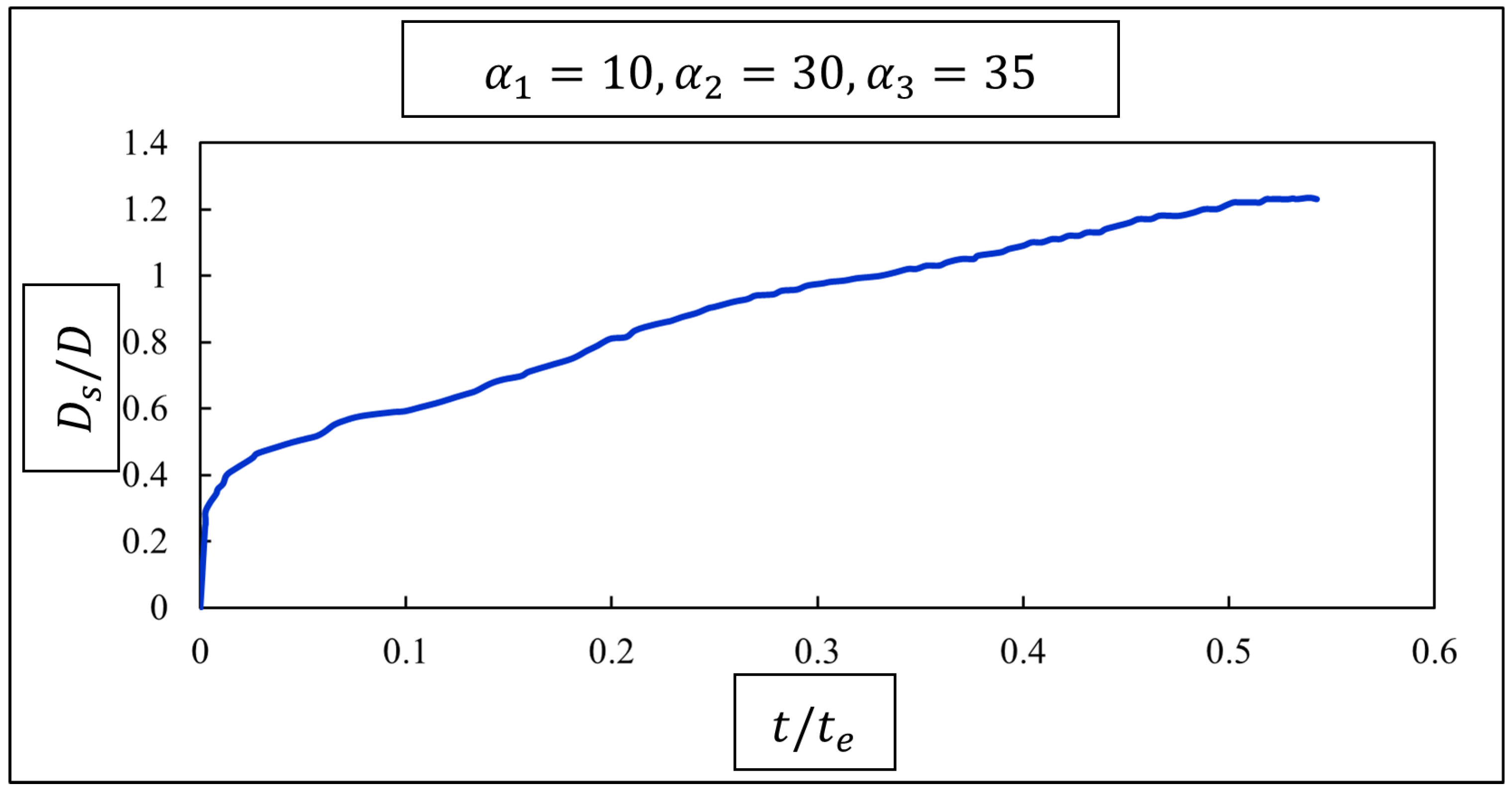
Consistent with Section 2.1, all experiments were performed under constant hydraulics (fixed flow depth, discharge, sediment size, and Froude number). We therefore formulate scour evolution using dimensionless variables so that model coefficients are not tied to units and the temporal progression is comparable across runs (refer to Figure 2).
In the most general form for this experimental program, the relative scour depth at time t can be written as a function of the dimensionless time and vane–geometry groups:
s D = F t t e , α , z D , e D , a D , L H , n ,
where s is the instantaneous scour depth, D is the pier diameter, t e is the equilibrium time, α denotes vane installation angle(s), z is the transverse offset, e is the longitudinal spacing, a is the lateral spacing, L / H is the vane aspect ratio, and n is the number of vanes (rows).
Following Shojaei et al. [46], the geometric and layout parameters were fixed at their reported optimum for scour mitigation ( a = 0 , e = 6 cm , z = 9 cm , n = 6 , and L / H = 3 ) and held constant throughout our dataset (see Table 2 and Figure 1). Under these controlled conditions, the only free geometric variables are the installation angles of the three vane rows ( α 1 , α 2 , α 3 ) and the temporal progression captured by t / t e . Accordingly, Equation (1) specializes to the compact four-input formulation used in this study:
s D = f t t e , α 1 , α 2 , α 3 ,
where α i is the installation (attack) angle of the submerged vanes in rows 1–3 (as defined by Shojaei et al. [46]); this reduction is deliberate: by holding hydraulics and non-angle geometry constant, we isolate and quantify the role of vane angles on scour evolution while describing time with the dimensionless ratio t / t e ( 0 1 ).
We train and evaluate three predictive models on Equation (2): (i) a symbolic regression via gene expression programming, (ii) an ε -SVR model, and (iii) a feed-forward ANN, all using the same inputs t t e , α 1 , α 2 , α 3 and response s D . Configuration and hyperparameter details are provided in Section 3, and performance comparisons are summarized.

2.3. Limitations and Scope

The present formulation deliberately isolates the role of vane installation angles by holding hydraulics and non-angle geometry constant across experiments (fixed flow depth, discharge, sediment size, and Froude number; see Section 2.1). Under these controlled conditions, the reduced, dimensionless mapping
s / D = f t / t e , α 1 , α 2 , α 3
provides a transparent and internally valid relation for the tested regime. We explicitly caution that transfer to other flow or sediment conditions requires recalibration or retraining with expanded inputs (e.g., flow depth, velocity, D 50 ). We identify this as a priority for future work.

3. Model Configurations and Training Protocol

3.1. GEP Configuration

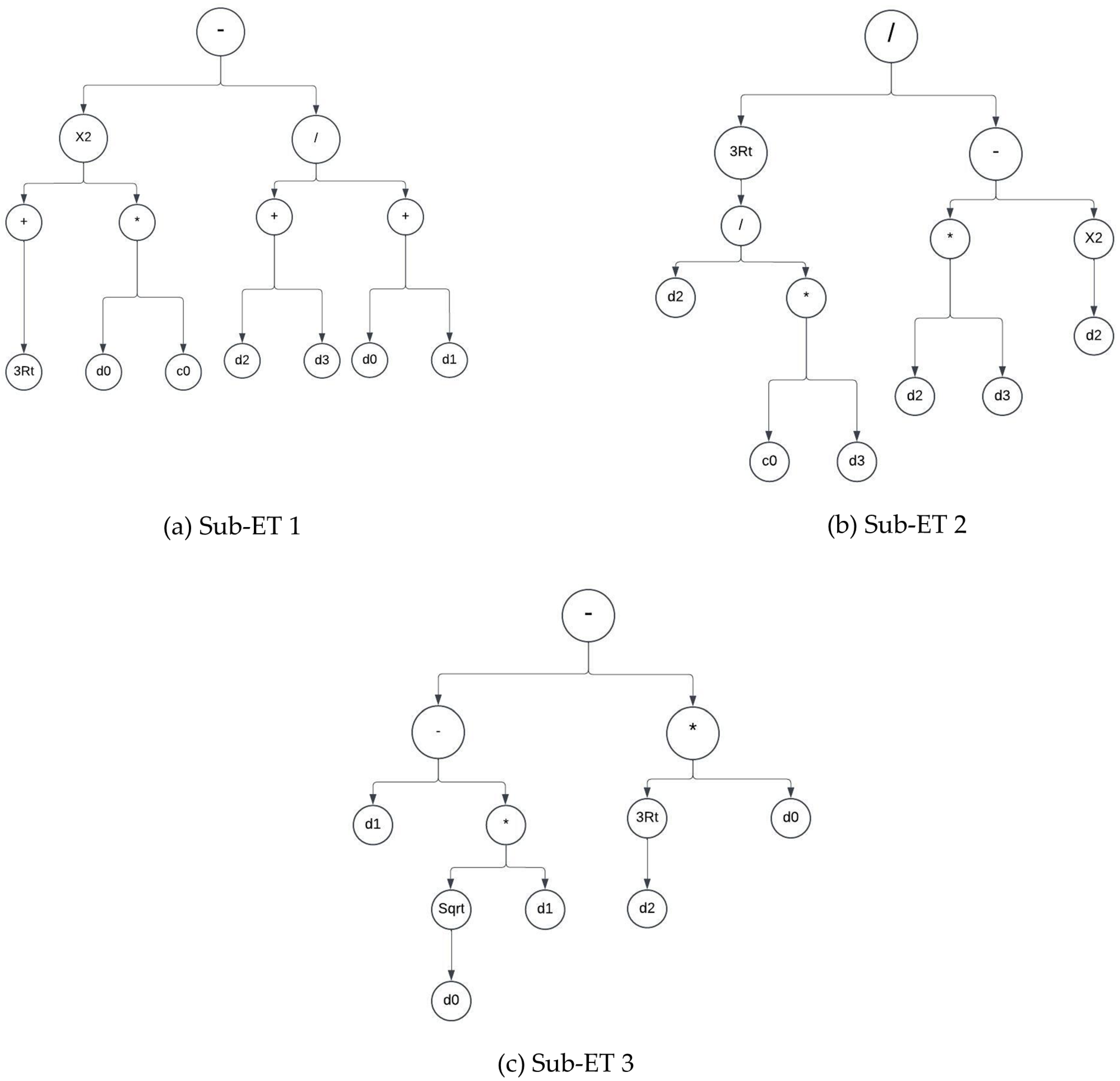
We employ gene expression programming (GEP) [47] as a symbolic regression tool to learn the mapping in Equation (2), from the four inputs ( t / t e , α 1 , α 2 , α 3 ) to the response s / D , and to obtain an explicit closed-form relation. GEP was implemented in GeneXproTools 4.0 on the same 70/30 train/test split described in Section 2.1. The overall flow of GEP is shown in Figure 3, and the expression tree of the best individual is shown in Figure 4.
  • Configuratio2 (problem-specific).
Chromosomes comprise g = 3 genes (head size =   8 ) linked by multiplication and evolve over a population of 30 chromosomes. The function set was chosen to capture smooth hydraulic nonlinearities:
{ + , , × , ÷ , · , ( · ) 2 , ( · ) 3 , · 3 } .
Fitness was measured by relative root squared error (RRSE). Genetic operator rates were set as follows: mutation = 0.044 ; inversion = 0.10 ; one-point recombination = 0.30 ; two-point recombination = 0.30 ; gene recombination = 0.10 ; gene transposition = 0.10 ; insertion sequence (IS) transposition = 0.10 ; root insertion sequence (RIS) transposition = 0.10 . Terminals consisted of the four inputs ( t / t e , α 1 , α 2 , α 3 ) and automatically defined constants as provided by the software. The best-of-run individual yields the closed-form regression relation (Equation (3)), which is evaluated alongside SVR and ANN on the identical held-out test set.
s D = G t t e , α 1 , α 2 , α 3 ,
Here, let G : R 4 R denote the GEP-derived regression mapping of the best-of-run individual.

3.2. SVR Configuration

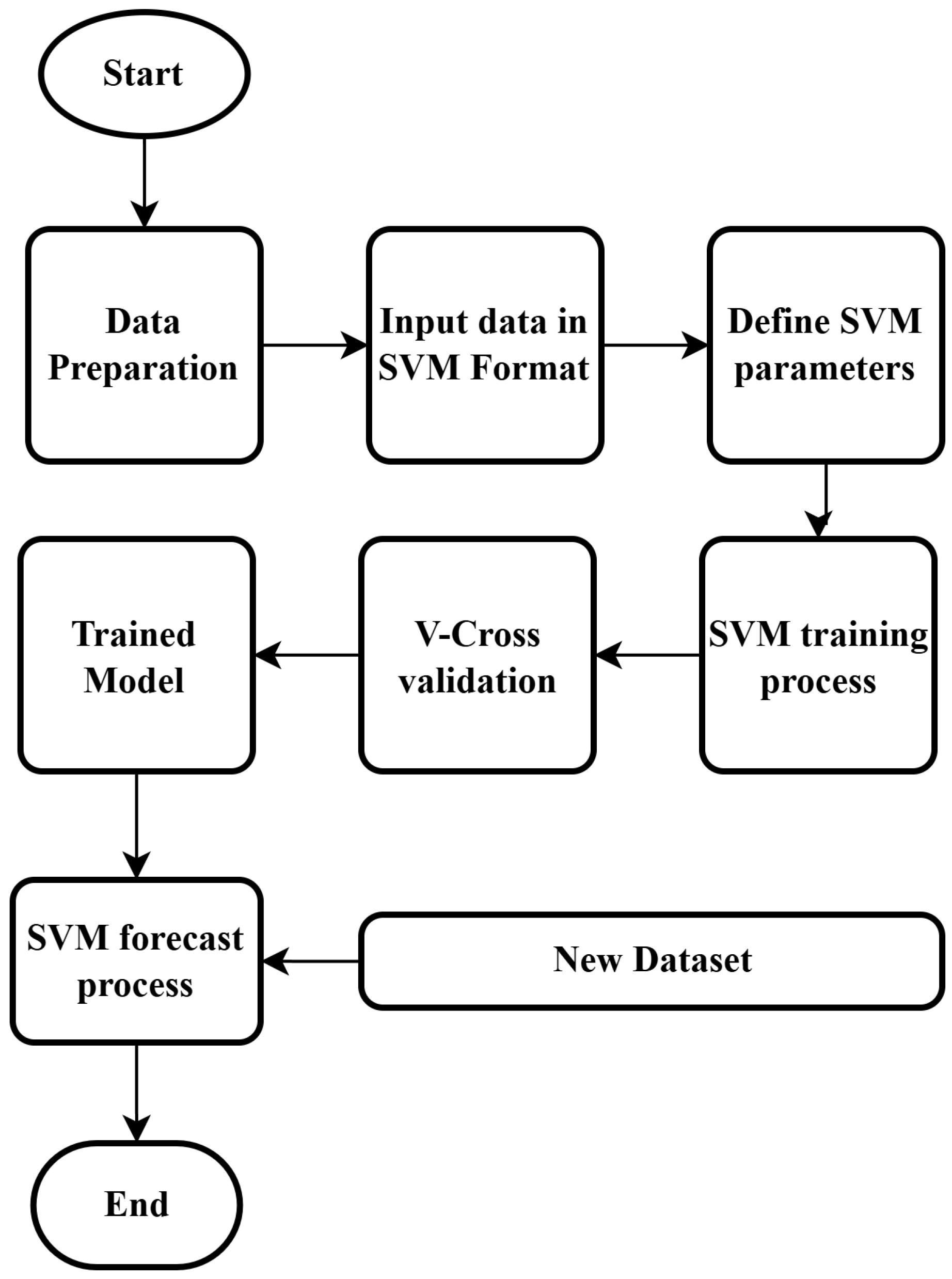
We use ε –support vector regression (SVR) [48] to learn the mapping in Equation (2) from the four inputs ( t / t e , α 1 , α 2 , α 3 ) to the response s / D . All experiments share constant hydraulics (Section 2.1), and the inputs are dimensionless; no additional feature scaling was required. SVR was trained on the same 70/30 train/test split as the other models, and its skill is reported in Table 3. Figure 5 presents the workflow of the ε –SVR used in this study.
  • Configuration (problem-specific).
We adopt the radial basis function (RBF) kernel with parameters
C = 110 , ε = 2.65 , γ = 5.5 ,
and the standard ε –insensitive loss. These settings were selected for this dataset to balance bias and variance and are applied identically to the train/test partition used for GEP and ANN. Software: STATISTICA 14.0 (RBF–SVR).
  • Notes on kernels (for context).
Although we use the RBF kernel in this work, common SVR kernels are listed below for reference.

3.3. ANN Configuration

We employ a feed-forward backpropagation (FFBP) artificial neural network to approximate the mapping in Equation (2) from the four inputs ( t / t e , α 1 , α 2 , α 3 ) to the response s / D . The model was implemented in MATLAB v2024b using the same 70/30 train/test split described in Section 2.1; its predictive skill is reported in Table 3.
  • Configuration (problem-specific).
The network comprises an input layer with four neurons, a single hidden layer with 15 neurons using the logistic–sigmoid activation (LOGSIG), and a linear output neuron for regression. Although the inputs are dimensionless, we apply min–max normalization to [ 0 ,   1 ] for numerical stability during training. The loss function is mean squared error (MSE). We train the network with the Levenberg–Marquardt algorithm (TRAINLM); the adaptive learning function is LEARNGD. Default MATLAB initialization is used, and the identical train/test partition is applied as for GEP and SVR.
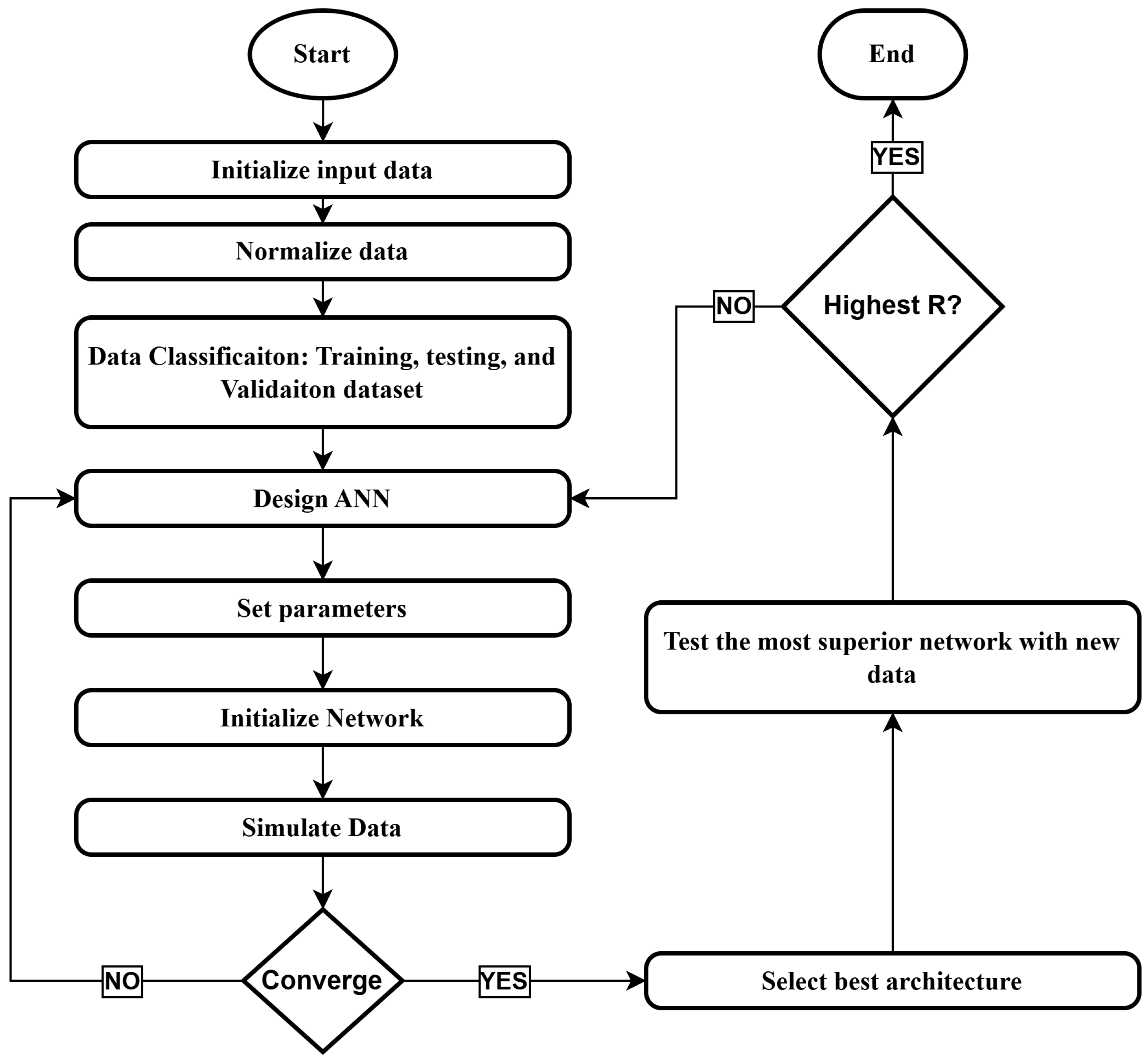
In Figure 6, R denotes the Pearson correlation coefficient between the ANN’s predicted and observed s / D on the validation set, and the decision step “Highest R?” corresponds to selecting the architecture with the most extensive validation R (equivalently R 2 ), subject to consistency with RMSE/MAE.

4. Results and Discussion

A summary of the results derived from simulating the temporal variations in the bed profile using three distinct models, namely SVM, GEP, and ANN, is presented in Table 4. Based on the evaluation of performance indicators, the model exhibiting the lowest RMSE and MAE, along with the highest R 2 and D s D DDR ( max ) , signifies optimal model performance.
In addition to aggregate errors (RMSE, MAE) and goodness-of-fit ( R 2 ), we report the design-oriented indicator DDR ( max ) max t ( D s / D ) , the peak relative scour over time. In bridge–pier scour assessment, a predicted DDR ( max ) that is slightly greater than the observed peak is considered conservative (safer) and thus satisfactory, whereas underprediction would be non-conservative. We nonetheless cross-check that such conservatism is not excessive by examining RMSE/MAE across the full time series.
Based on the numerical values presented in Table 4, it is evident that the GEP model demonstrates superior performance compared to other models. The performance evaluation metrics, including RMSE, MAE, R 2 , and D s D DDR ( max ) , were computed for both training and test phases. The corresponding values for the training phase were determined as ( 0.0864 , 0.0681 , 0.9237 , 4.2501 ) , while for the test phase, the values were calculated as ( 0.0729 , 0.0641 , 0.9143 , 4.9405 ) .
The implementation of the GEP model was performed using GeneXprotools 4.0 software. Table 5 provides an overview of the tuning parameters employed in this model, while Figure 5 illustrates the tree representation of the GEP model output. The mathematical operators employed in this model encompassed addition (+), subtraction (−), multiplication (×), division (/), square root (Sqrt), square ( x 2 ), cube ( x 3 ), and cube root (3Rt).
Because GEP yields a symbolic regression relation, as shown in Equation (3), Table 4 provides a direct head-to-head comparison of that regression with SVR (RBF) and ANN (FFBP) on the identical 70/30 split and inputs ( t / t e , α 1 , α 2 , α 3 ) .
The mathematical expression of the GEP model output can be presented as shown in Equation (4):
D s D = 3 d 1 + 9.45 d 0 2 d 2 d 3 d 0 + d 1 × 3 d 2 3.105 d 3 d 2 d 3 × d 1 d 1 d 0 d 0 3 d 2
where d 0 stands for t / t e , and d 1 , d 2 , and d 3 are the installation angles of the first to third rows of submerged vanes (in degrees).
However, SVM and ANN models can also be considered for evaluation as they have produced acceptable results. The temporal variations in the bed profile were simulated utilizing the SVM model through the STATISTICA software. This particular model represents the second order of the simulation process. The ensuing results encompassing the performance evaluation metrics, namely RMSE, MAE, R 2 , and D s D DDR ( max ) , were acquired for both the training and test phases. The computed values for the training phase were determined as follows: RMSE = 0.2239 , MAE = 0.1692 , R 2 = 0.7817 , and D s D DDR ( max ) = 1.8964 . Subsequently, the values obtained for the testing phase were RMSE = 0.2141 , MAE = 0.1743 , R 2 = 0.6722 , and D s D DDR ( max ) = 2.2346 . The tuning parameters of the SVM model were derived as C = 110 , ε = 2.65 , and γ = 5.5 . Among the various kernel functions available, the RBF kernel was deemed the most optimal choice for accurately modeling the outputs in this context.
In addition, the ANN model achieved the third rank in terms of performance. The simulation using ANN was conducted with the aid of MATLAB software. The computed values of the performance evaluation metrics (RMSE, MAE, R 2 , D s D DDR ( max ) ) for the training phase were found to be 0.1531, 0.0794, 0.7359, and 1.6720, respectively. Similarly, in the testing phase, the corresponding values for these indicators were determined as 0.1476, 0.0852, 0.7721, and 2.1992, respectively. Figure 5 illustrates the architecture of the neural network employed in this study; it depicts the structure of the desired neural network configuration.
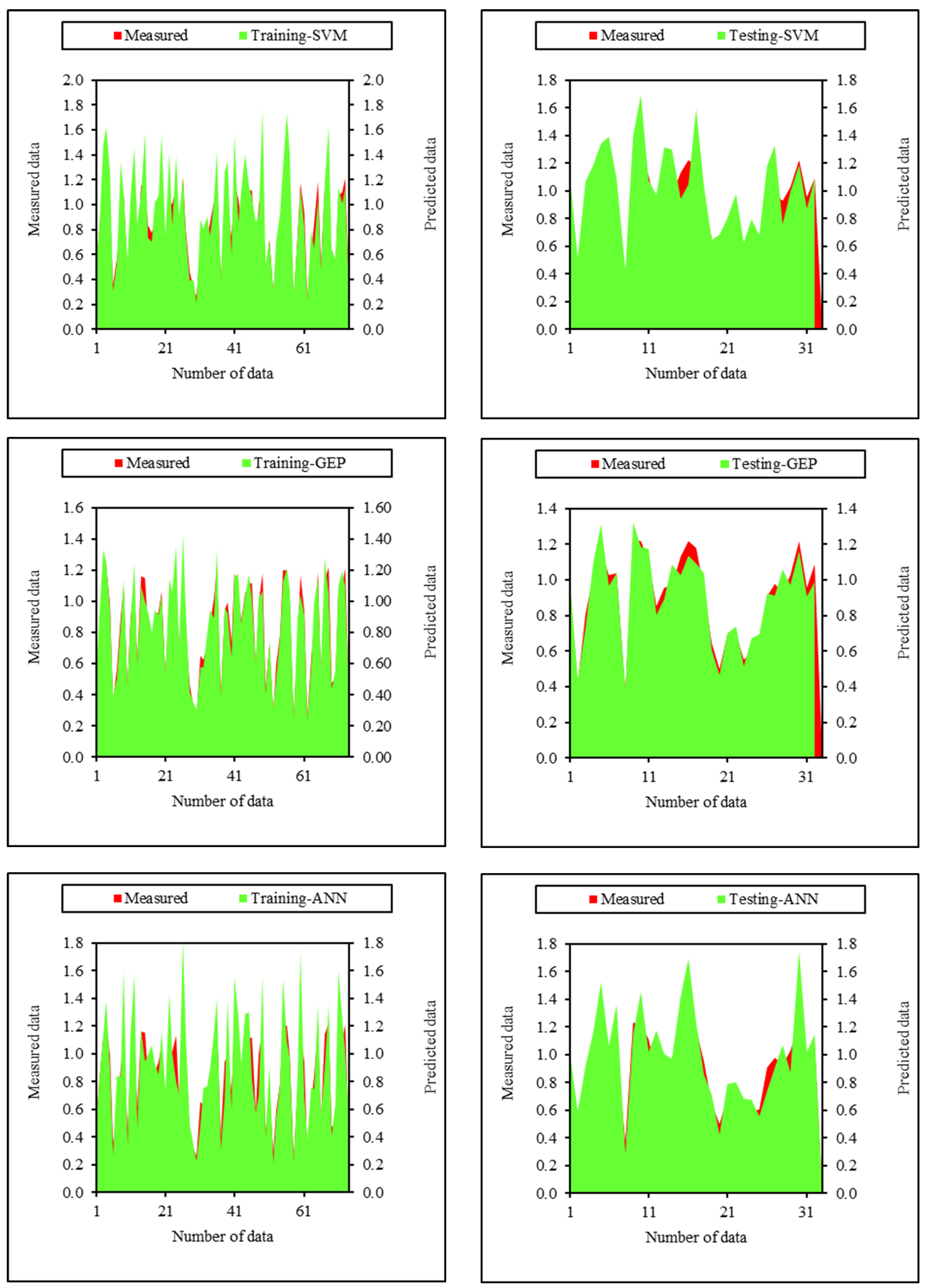
Graphical comparisons are employed to assess and compare the outputs of the MLMs involved. Figure 7 presents an area diagram that is utilized to present the performance of the MLMs. This figure is generated and displayed for both the training and testing phases of the MLMs. The correspondence between the green and red graphs within these plots represents the performance of each respective model. The outcomes depicted in this graphical representation align with the numerical results obtained in Table 3. It is observed that the GEP model exhibits the lowest discrepancy, while the ANN model demonstrates the highest level of discrepancy among the models.
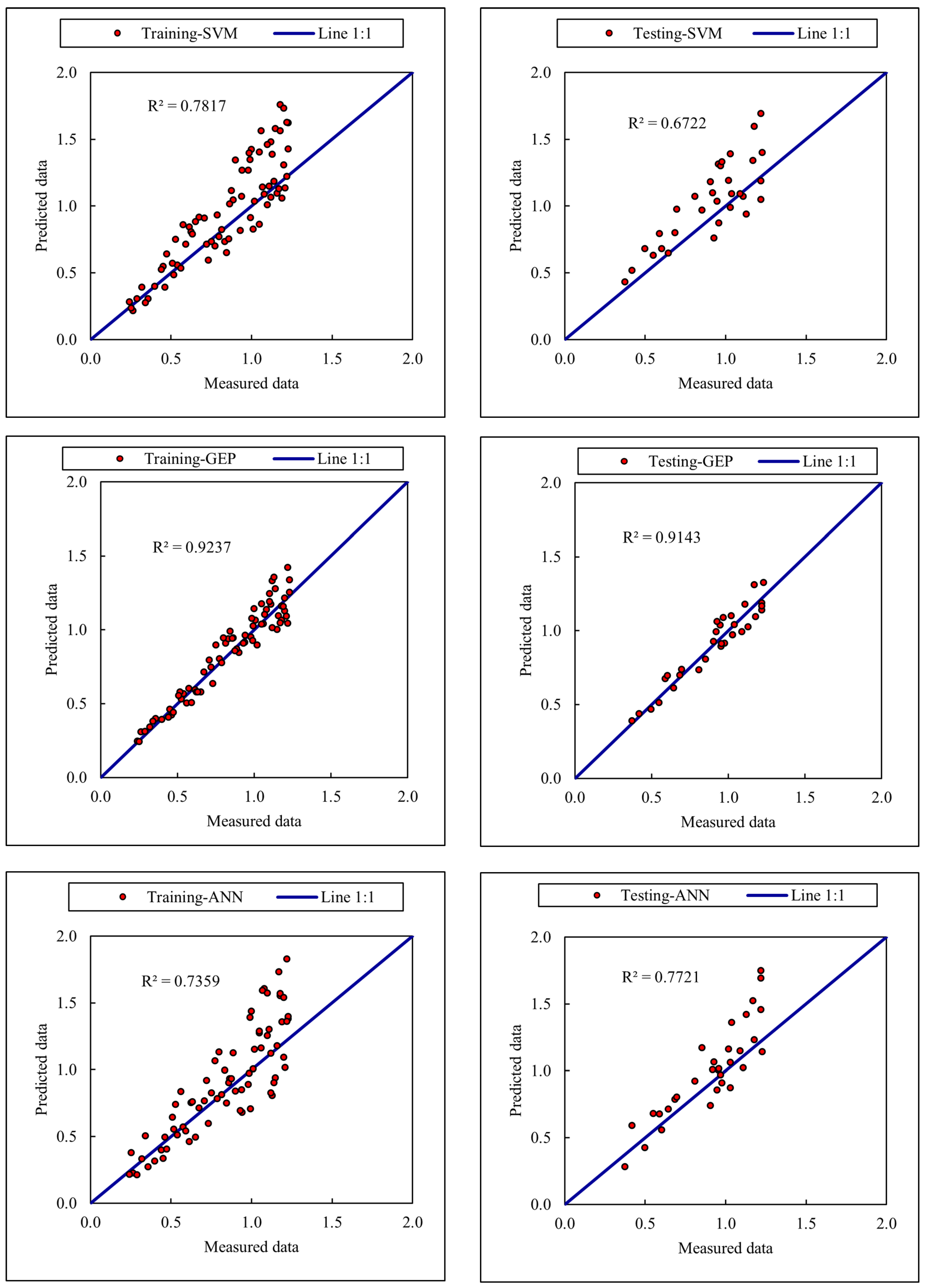
Figure 8 illustrates the coefficient of determination curves for both the training and testing stages of all three models. Among the graphical representations employed to assess model performance, this diagram visualizes the distribution of the observed and calculated values of the output parameter in relation to a line with a slope of 1:1. A smaller dispersion of data points around this line indicates better model performance, while a larger dispersion suggests lower accuracy.
The numerical measure used to evaluate data distribution is the coefficient of determination ( R 2 ). A higher R 2 value signifies a smaller distribution of points around the 1:1 line. It is evident from this figure that the GEP model outperforms the other two models, as it exhibits superior performance. The dispersion of data points around the 1:1 line is notably smaller for the GEP model, indicating its higher accuracy compared to the other models.
All values reported in Figure 7 and Figure 8 correspond to the relative scour–depth ratio D s / D .
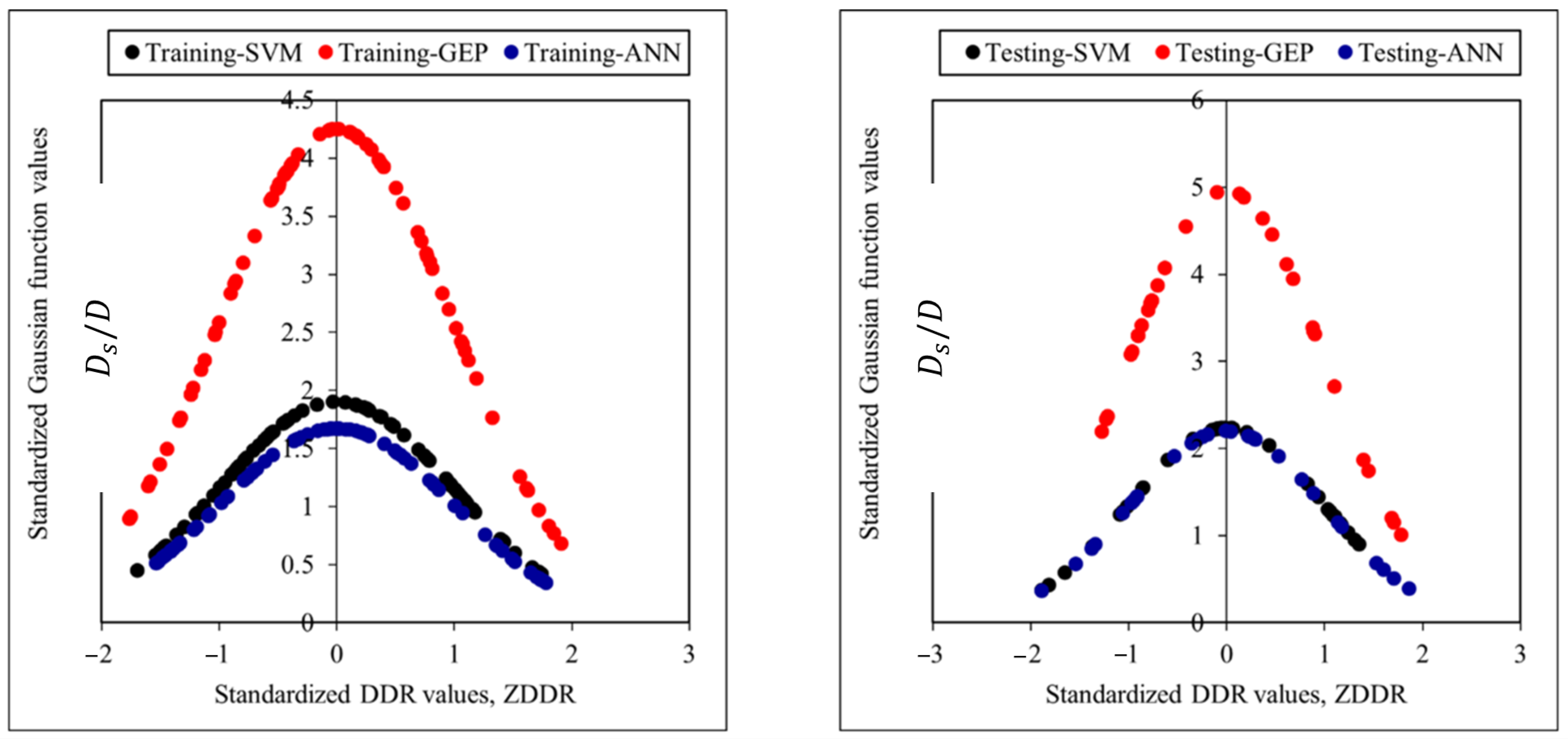
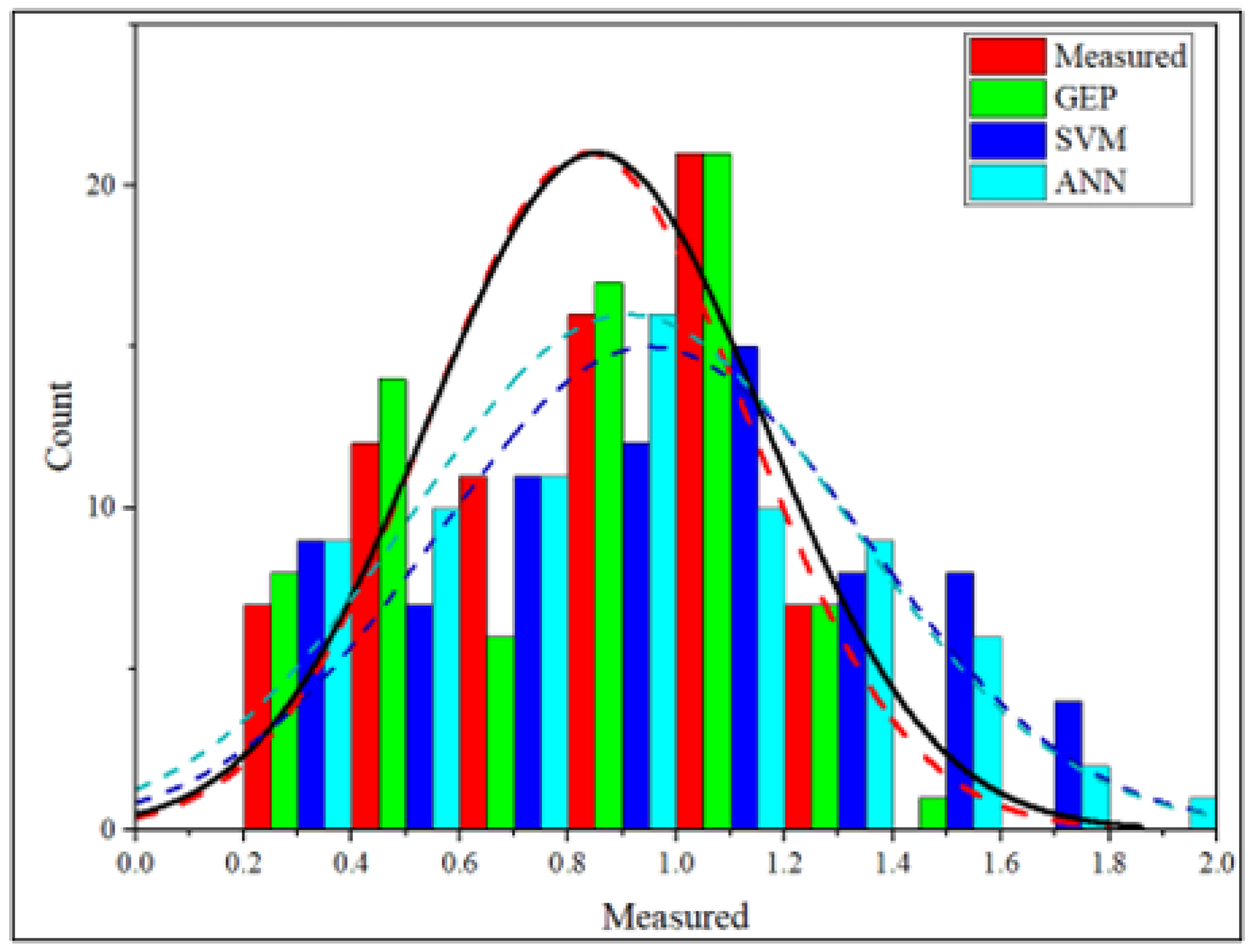
In addition, Figure 9 illustrates the graphical comparison of the performance of MLMs with respect to the distribution of the DDR index. Two attributes of this curve highlight superior model performance: (i) a narrower distribution curve and (ii) the maximum value on the vertical axis. These curves are presented for both the training and testing stages, allowing for a comprehensive assessment of model performance.
The analysis of Figure 9 confirms that the GEP model exhibits the best performance. This conclusion is supported by two observations: first, the distribution curve of the GEP model is narrower compared to the other models. Second, the GEP model achieves the maximum values of 4.25 and 4.94 on the vertical axis during the training and testing steps, respectively. In contrast, the SVM and ANN models are ranked lower in terms of performance based on this evaluation.
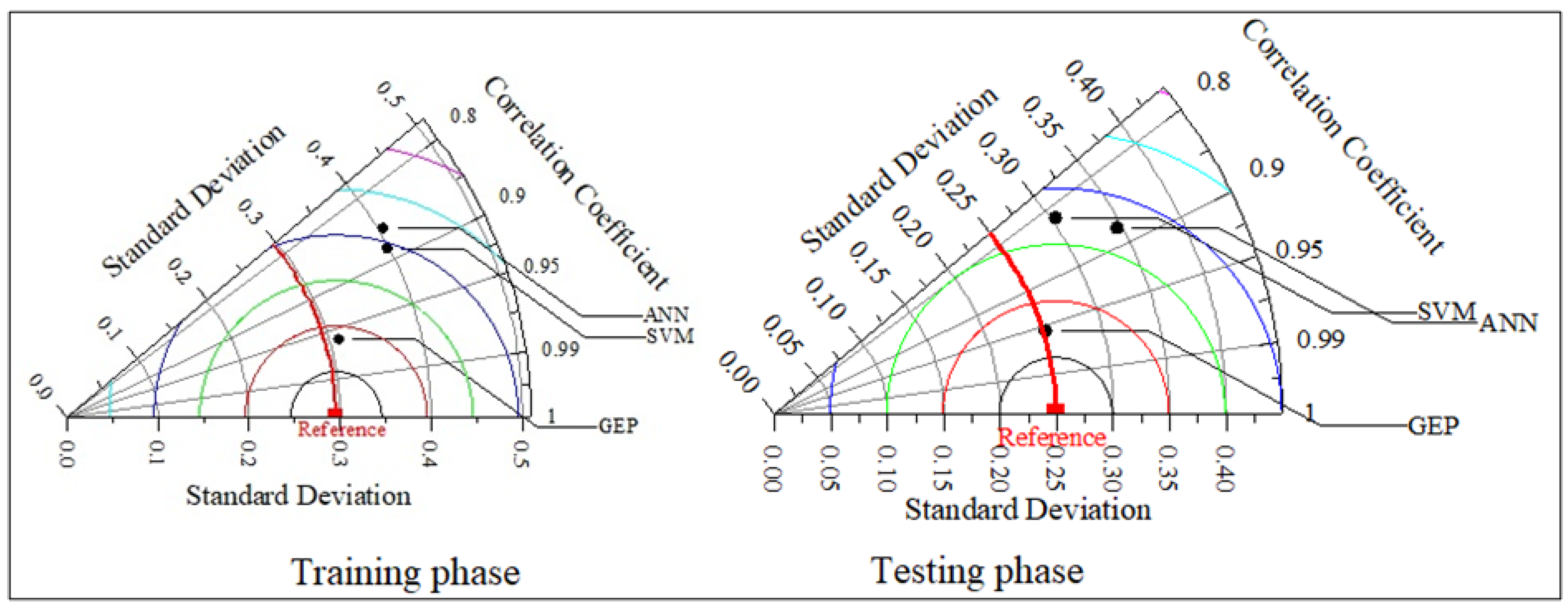
The Taylor diagram developed for the training and testing phases is given in Figure 10. The figure illustrates the superiority of the GEP model based on the features of the aforementioned diagram.
Figure 11 presents a comprehensive visual comparison between the measured (observed) bed profiles and profiles predicted by the GEP model at the cylindrical bridge pier location across various stages of scour development. During the initial formation of the scour hole (early time steps), the predicted profile from the GEP model closely aligns with the observed measurements, indicating the model’s strong capability to capture incipient sediment erosion dynamics and early vortex formation around the pier.
However, as the scour hole progressively widens and deepens toward equilibrium conditions ( t t e ), a discernible divergence emerges between the predicted and observed profiles. This growing disparity is attributed to the escalating complexity of sediment–fluid interactions, including intensified turbulence and chaotic secondary flow structures that challenge precise simulation.
The model’s performance, reinforced by its superior metrics (RMSE =   0.0729 , R 2 = 0.9143 in testing), underscores its utility in forecasting scour-related vulnerabilities and optimizing mitigation strategies such as submerged vane deployment before significant damage occurs.
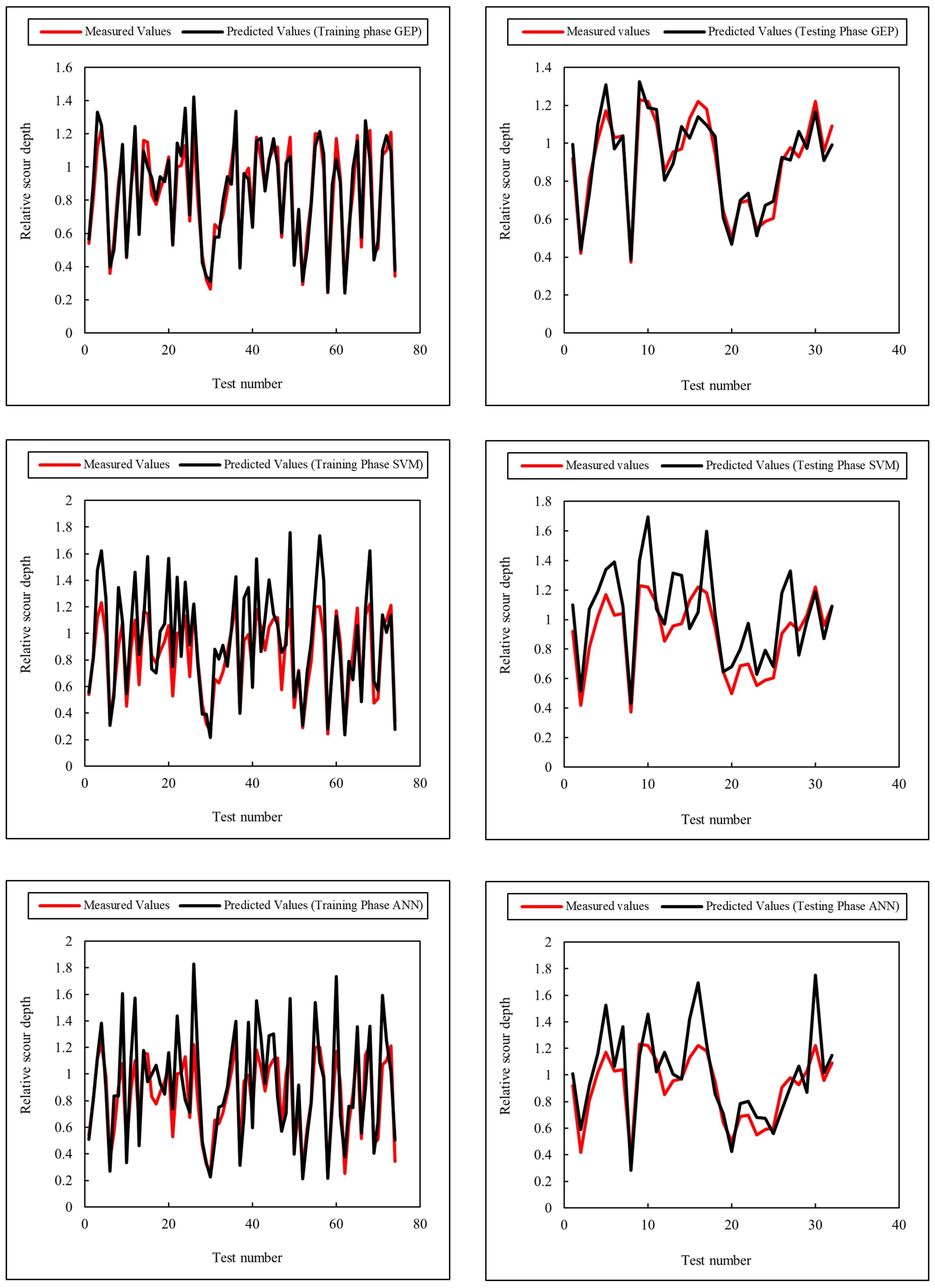
To facilitate a more qualitative comparison among the outputs of the three models, Figure 12 illustrates the extent of concordance between observational and computational data during the training and testing phases. It is evident from these figures that the discrepancies between observed and predicted values are significantly greater in the SVM and ANN models compared to the GEP model.
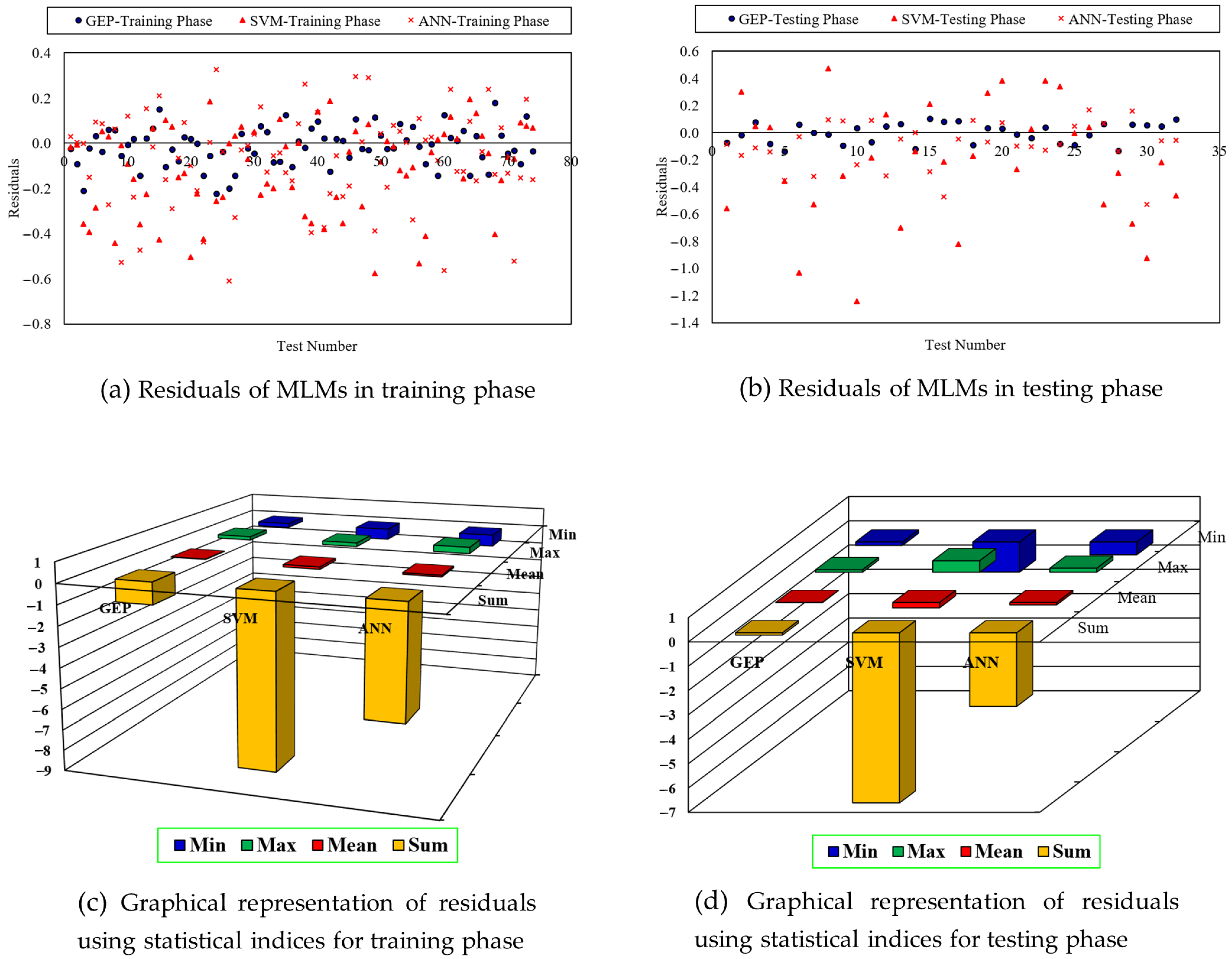
Figure 13a,b present the residual values derived from the outputs of the three models during both the training and testing phases. This figure indicates that the GEP model exhibits substantially lower residual error compared to the SVM and ANN models.
The minimum, maximum, average, and total residual error values during the training phase for the GEP, SVM, and ANN models are as follows: GEP (−0.2237, 0.1781, −0.0145, −1.0757), SVM ( 0.5770 , 0.1944 , 0.1144 , 8.4625 ) , and ANN (−0.6088, 0.3254, −0.0739, −5.4694).
During the testing phase, these values are GEP ( 0.1392 , 0.1040 , 0.0029 , 0.0930 ) , SVM ( 1.2404 , 0.4712 , 0.2184 , 6.9884 ) , and ANN ( 0.5295 , 0.1658 , 0.0947 , 3.0291 ) .
In addition, Figure 13c,d provide qualitative comparisons of the residual properties for the three models during both the training and testing phases. This figure clearly highlights the substantial differences in accuracy among the outputs of the GEP, SVM, and ANN models.
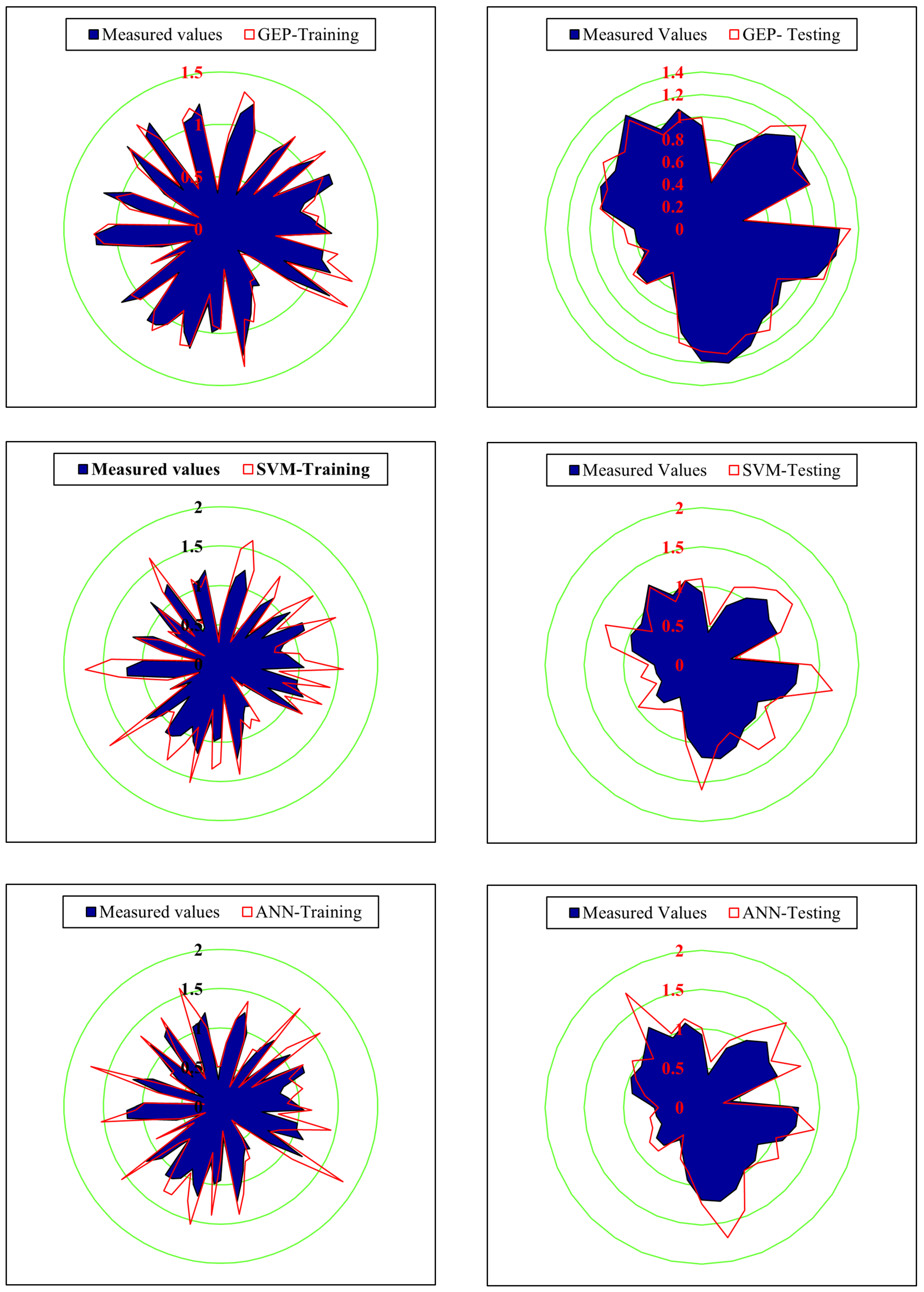
Figure 14 employs a radar plot to visually compare the alignment of predicted versus observed relative scour depths D s D across the SVM, GEP, and ANN models during both training and testing phases. The GEP model consistently exhibits the closest alignment to the center of the plot (representing perfect agreement with observed values) across all scour depth ranges, confirming its superior accuracy as quantified by performance metrics (e.g., testing RMSE =   0.0729 , R 2 = 0.9143 ).
For instance, at low-to-moderate scour depths, GEP’s predictions nearly overlap with observational benchmarks, reflecting its strength in capturing early-stage scour dynamics. However, all models display a progressive decline in accuracy as relative scour depth increases, evidenced by radial expansion (increasing distance from the plot center) at higher values. This error escalation reaches up to 20 to 25 % for SVM and ANN under severe scouring conditions, while GEP maintains closer alignment (≈10% error), attributed to escalating turbulence and sediment–fluid interactions that challenge predictive precision.
Finally, the distribution of predicted versus observed data, as shown in Figure 15, indicates that the GEP model achieves a very good fit between its simulated data and the observed values.
Therefore, the comprehensive comparison analysis suggests that the GEP model is the best among the tested models. Comprehensive comparison analysis indirectly evaluated the black-box nature of the MLMs.
The superior performance of the GEP model (testing: RMSE = 0.0729 , R 2 = 0.9143 ) aligns with recent trends in ML-based scour prediction, where symbolic regression techniques increasingly outperform conventional models in capturing complex hydraulic interactions. For instance, Roshni (2023) reported ANFIS as optimal for live-bed scour prediction [30], while Kumar et al. (2023) found ensemble methods effective for time-dependent scour [29]. Our results extend these findings by demonstrating GEP’s advantage in simulating temporal bed profile evolution under submerged vane intervention, a scenario not explicitly addressed in prior ML studies (Table 1). The explicit formulation derived from GEP (Equation (4)) provides physical interpretability missing in black-box models like ANN and SVM, echoing Zhang et al.’s (2023) emphasis on transparent equations for engineering applications [34]. Notably, our GEP accuracy ( R 2 > 0.91 ) exceeds SVM performances reported by Choi and Choi (2022) for cohesive beds ( R 2 0.85 ) and ANN results by [41] for pier scour ( R 2 0.82 ). This enhancement likely stems from GEP’s ability to model nonlinear interactions between installation angles ( α 1 , α 2 , α 3 ) and dimensionless time ( t / t e ), variables previously unintegrated in scour simulations. This study thus bridges a critical gap between empirical scour mitigation research (e.g., [6]) and ML-driven hydraulic modeling, establishing a framework for optimizing submerged vane configurations via data-driven approaches.
While GEP’s explicit equation (Equation (4)) enables the direct interpretation of scour dynamics, such as the nonlinear role of vane angles (e.g., d 1 3 terms) and time dependency ( d 0 ), SVM and ANN models lack equivalent physical transparency. The SVM’s kernel transformations (e.g., RBF) map inputs into high-dimensional spaces where feature interactions become intractable, obscuring cause–effect relationships. Similarly, ANN’s layered transformations (e.g., weighted sums and LOGSIG activations) create a black box that resists mechanistic interpretation. Though these models achieve reasonable predictive accuracy (Table 4), their inability to distil hydraulic principles limits utility for scour mitigation design, where understanding why a configuration reduces scour is as critical as prediction itself.
Although the present study establishes the superiority of GEP in simulating temporal scour profiles, it further clarifies the physical linkages between model inputs and scour dynamics. The submerged vane angles ( α 1 , α 2 , α 3 ) directly disrupt the horseshoe vortex by generating secondary currents that redistribute bed shear stress, thereby reducing sediment entrainment capacity near the pier. Specifically, optimal angles (40–60 °) expand the zone of influence, diverting sediment transport pathways, as confirmed by empirical studies [6,8]. Concurrently, the dimensionless time ratio ( t / t e ) encodes transient evolution toward equilibrium scour depth, capturing feedback between flow duration and sediment mobilization. The GEP model’s explicit equation (Equation (4)) quantifies these nonlinear interactions, revealing how cube-root transformations of vane angles amplify their hydraulic impact, a finding aligned with vortex coherence theory. This physics-informed interpretation positions our MLM framework as both a predictive tool and a diagnostic lens for scour mitigation design.

5. Conclusions

The fundamental framework of the presented investigation revolves around the simulation of temporal variations in bed sediment profile at the bridge pier, employing three MLMs, namely SVM, GEP, and ANN. The research findings demonstrate that all three models effectively simulate temporal changes in scour profiles at the bridge base. However, the GEP model exhibits superior accuracy compared to the other two models. Specifically, the optimal GEP model with a three-gene structure achieved the best performance metrics during both the training and testing phases.
During the training phase, the optimal GEP model yielded the following metrics: RMSE = 0.0864 , MAE = 0.0681 , R 2 = 0.9237 , and ( D s / D ) DDR ( max ) = 4.25 . Subsequently, during the testing phase, the model maintained high performance with RMSE = 0.0729 , MAE = 0.0641 , R 2 = 0.9143 , and ( D s / D ) DDR ( max ) = 4.94 . These results confirm that the GEP model outperforms the SVM and ANN models.
Because Equation (4) is a closed-form expression obtained for the constant hydraulic regime studied here, its use outside this regime should be accompanied by recalibration with additional hydraulic predictors.
The results of this study can be widely applied in premonitory assessments of bridges under scour-induced threats. In addition, ongoing climate change, as discussed above, directly impacts the stability of bridges. Therefore, the outcomes of this research may be integrated into climate change impact analyses. Future investigations are proposed to incorporate climate change scenarios into simulations of bed profile evolution under bridges. In particular, forthcoming work will integrate GEP-predicted relative scour depth into flood risk assessment models, thereby enabling the evaluation of pier vulnerability under projected climate-induced flow regime shifts (e.g., intensified floods) to inform adaptive bridge designs.
While this study demonstrates GEP’s superior accuracy in simulating temporal bed profile changes under submerged vanes, we explicitly acknowledge that its findings hold conditional validity, restricted to the tested hydraulic conditions and uniform sediment. This deliberate simplification enabled the isolation of vane angle effects but inherently limits direct extrapolation to natural systems exhibiting transient flows, graded sediments, or alternative pier geometries. Ongoing research aims to extend the framework’s applicability by incorporating variable discharges, flood hydrographs, and nonuniform sediments under realistic field scenarios.

Supplementary Materials

The following supporting information can be downloaded at: https://www.mdpi.com/article/10.3390/hydrology12090238/s1, Table S1: Sample values of relative scour depth ( D s / D s ) for training and testing subsets.

Author Contributions

A.M.: conceptualization of methodology, experimentation, writing of the draft; F.A.K.: software and methodology, data collection; N.R.: analysis, writing of the draft; U.R.: interpretation of results, review and writing, conceptualization; M.F.: draft preparation, software and methodology; H.M.A.: revision of methodology and draft. All authors have read and agreed to the published version of the manuscript.

Funding

This research received no external funding.

Data Availability Statement

A PDF with the sample train/test table of relative scour–depth ratios ( D s / D ) is provided in the Supplementary Materials. The full dataset used in this study is available from the corresponding author upon reasonable request for research purposes.

Conflicts of Interest

The authors declare no conflicts of interest.

References

  1. Raudkivi, A.J. Functional trends of scour at bridge piers. J. Hydraul. Eng. 1986, 112, 1–13. [Google Scholar] [CrossRef]
  2. Ettema, R.; Nakato, T.; Muste, M.V.I. An Illustrated Guide for Monitoring and Protecting Bridge Waterways Against Scour; Technical report; Iowa Highway Research Board Project TR-515; IIHR-Hydroscience & Engineering, University of Iowa: Iowa City, IA, USA, 2006. [Google Scholar]
  3. Chiew, Y.M. Scour Protection at Bridge Piers. J. Hydraul. Eng. 1992, 118, 1260–1269. [Google Scholar] [CrossRef]
  4. Ettema, R.; Constantinescu, G.; Melville, B.W. Flow-Field Complexity and Design Estimation of Pier-Scour Depth: Sixty Years Since Laursen and Toch. J. Hydraul. Eng. 2017, 143, 03117006. [Google Scholar] [CrossRef]
  5. Zarrati, A.R.; Gholami, H.; Mashahi, M.B. Application of collar to control scouring around rectangular bridge piers. J. Hydraul. Res. 2004, 42, 97–103. [Google Scholar] [CrossRef]
  6. Hamidi, M.; Sadeqlu, M.; Khalili, A.M. Investigating the design and arrangement of dual submerged vanes as mitigation countermeasure of bridge pier scour depth using a numerical approach. Ocean Eng. 2024, 299, 117270. [Google Scholar] [CrossRef]
  7. Odgaard, A.J.; Kennedy, J.F. River-bend bank protection by submerged vanes. J. Hydraul. Eng. 1983, 109, 1161–1173. [Google Scholar]
  8. Ebrahimi, T.; Hamidi, M.; Rahmani Firoozjaiee, A.; Khavasi, E. Numerical investigation of scour around a cylindrical pier in laboratory scale using Euler-Lagrange approach. Amirkabir J. Mech. Eng. 2021, 53, 411–426. [Google Scholar]
  9. Omara, H.; Ookawara, S.; Nassar, K.A.; Masria, A.; Tawfik, A. Assessing local scour at rectangular bridge piers. Ocean Eng. 2022, 266, 112912. [Google Scholar] [CrossRef]
  10. Mashahir, M.; Zarrati, A.R.; Tabarestani, M.K. Evaluation of collar efficiency to prevent scouring around cylindrical bridge piers under live bed condition. J. Hydro-Environ. Res. 2024, 52, 17–25. [Google Scholar] [CrossRef]
  11. Mowla, Q.A.E.; Ahmari, H. Experimental Study of Flow Characteristics and Geometry of Scour Hole around Cylindrical Piers Subject to Wave and Current. J. Waterw. Port Coast. Ocean Eng. 2024, 150, 04023020. [Google Scholar] [CrossRef]
  12. Javidi Vahdati, V.; Ahmadi, A.; Abedini, A.; Heidarpour, M. Efficacy of the Combined Use of Bed Sill and Sacrificial Piles to Control Local Scour Around Circular Bridge Piers. Shock Vib. 2024, 2024, 5527946. [Google Scholar] [CrossRef]
  13. Qi, H.; Yuan, T.; Zhao, F.; Chen, G.; Tian, W.; Li, J. Local Scour Reduction around Cylindrical Piers Using Permeable Collars in Clear Water. Water 2023, 15, 897. [Google Scholar] [CrossRef]
  14. Salemi, F.; Ghomeshi, M.; Bahrami Yarahmadi, M. Experimental Study of Transverse Waves Effects by Obstacles on Local Scour Around Cylindrical Pier Groups of Bridge. Iran. J. Sci. Technol. Trans. Civ. Eng. 2023, 47, 2409–2421. [Google Scholar] [CrossRef]
  15. Farooq, R.; Azimi, A.H.; Tariq, M.A.U.R.; Ahmed, A. Effects of hooked-collar on the local scour around a lenticular bridge pier. Int. J. Sediment Res. 2023, 38, 1–11. [Google Scholar] [CrossRef]
  16. Valela, C.; Rennie, C.D.; Nistor, I. Improved bridge pier collar for reducing scour. Int. J. Sediment Res. 2022, 37, 37–46. [Google Scholar] [CrossRef]
  17. Aly, A.M.; Dougherty, E. Bridge pier geometry effects on local scour potential: A comparative study. Ocean Eng. 2021, 234, 109326. [Google Scholar] [CrossRef]
  18. Raeisi, N.; Ghomeshi, M. Effect of bridge pier diameter on maximum depth of scour impacts on the environment. SN Appl. Sci. 2020, 2, 1974. [Google Scholar] [CrossRef]
  19. Tipireddy, R.T.; Barkdoll, B.D. Scour reduction by air injection at a cylindrical bridge pier: Experimental determination of optimal configuration. J. Hydraul. Eng. 2019, 145, 06018016. [Google Scholar] [CrossRef]
  20. Jahangirzadeh, A.; Basser, H.; Akib, S.; Karami, H.; Naji, S.; Shamshirband, S. Experimental and numerical investigation of the effect of different shapes of collars on the reduction of scour around a single bridge pier. PLoS ONE 2014, 9, e98592. [Google Scholar] [CrossRef]
  21. EL-Ghorab, E.A. Reduction of scour around bridge piers using a modified method for vortex reduction. Alex. Eng. J. 2013, 52, 467–478. [Google Scholar] [CrossRef]
  22. Zarrati, A.R.; Chamani, M.R.; Shafaie, A.; Latifi, M. Scour countermeasures for cylindrical piers using riprap and combination of collar and riprap. Int. J. Sediment Res. 2010, 25, 313–322. [Google Scholar] [CrossRef]
  23. Zarrati, A.R.; Nazariha, M.; Mashahir, M.B. Reduction of local scour in the vicinity of bridge pier groups using collars and riprap. J. Hydraul. Eng. 2006, 132, 154–162. [Google Scholar] [CrossRef]
  24. Chiew, Y.M. Local scour and riprap stability at bridge piers in a degrading channel. J. Hydraul. Eng. 2004, 130, 218–226. [Google Scholar] [CrossRef]
  25. Rathod, P.; Manekar, V.L. Comprehensive approach for scour modelling using artificial intelligence. Mar. Georesour. Geotechnol. 2023, 41, 312–326. [Google Scholar] [CrossRef]
  26. Le, X.H. Predicting maximum scour depth at sluice outlet: A comparative study of machine learning models and empirical equations. Environ. Res. Commun. 2024, 6, 015010. [Google Scholar] [CrossRef]
  27. Nandi, B.; Patel, G.; Das, S. Prediction of maximum scour depth at clear water conditions: Multivariate and robust comparative analysis between empirical equations and machine learning approaches using extensive reference metadata. J. Environ. Manag. 2024, 354, 120349. [Google Scholar] [CrossRef]
  28. Adib, A.; Tabatabaee, S.H.; Khademalrasoul, A.; Shoushtari, M.M. Recognizing of the best different artificial intelligence method for determination of local scour depth around group piers in equilibrium time. Arab. J. Geosci. 2020, 13, 1004. [Google Scholar] [CrossRef]
  29. Kumar, S.; Goyal, M.K.; Deshpande, V.; Agarwal, M. Estimation of time dependent scour depth around circular bridge piers: Application of ensemble machine learning methods. Ocean Eng. 2023, 270, 113611. [Google Scholar] [CrossRef]
  30. Roshni, T. Application of GEP, M5-TREE, ANFIS, and MARS for Predicting Scour Depth in Live Bed Conditions Around Bridge Piers. J. Soft Comput. Civ. Eng. 2023, 7, 24–49. [Google Scholar]
  31. Fujail, A.K.M. Hybrid Artificial Neural Network Model for Prediction of Scour Depth Upstream of Bridge Piers. In Soft Computing: Theories and Applications: Proceedings of SoCTA 2022; Springer Nature: Singapore, 2022; pp. 741–746. [Google Scholar]
  32. Kumar, L.; Afzal, M.S. Estimating pier scour depth under combined waves and current using boosting machine-learning models. Acta Geophys. 2024, 72, 1895–1911. [Google Scholar] [CrossRef]
  33. Choudhary, A.; Das, B.S.; Devi, K.; Khuntia, J.R. ANFIS-and GEP-based model for prediction of scour depth around bridge pier in clear-water scouring and live-bed scouring conditions. J. Hydroinform. 2023, 25, 1004–1028. [Google Scholar] [CrossRef]
  34. Zhang, W.; Rennie, C.D.; Nistor, I. A new model developed by multigene genetic programming for the temporal evolution of bridge pier scour. Can. J. Civ. Eng. 2023, 50, 549–559. [Google Scholar] [CrossRef]
  35. Choi, S.U.; Choi, S. Prediction of local scour around bridge piers in the cohesive bed using support vector machines. Ksce J. Civ. Eng. 2022, 26, 2174–2182. [Google Scholar] [CrossRef]
  36. Chou, J.S.; Nguyen, N.M. Scour depth prediction at bridge piers using metaheuristics-optimized stacking system. Autom. Constr. 2022, 140, 104297. [Google Scholar] [CrossRef]
  37. Ghodsi, H.; Khanjani, M.J. Application of improved GMDH models to predict local scour depth at complex bridge piers. Civ. Eng. J. 2020, 6, 69–84. [Google Scholar] [CrossRef]
  38. Li, Z.; Dai, G.; Du, S.; Ouyang, H.; Hu, T.; Liu, H.; Li, Z. Local Scour Depth Prediction of Offshore Wind Power Monopile Foundation Based on GMDH Method. J. Mar. Sci. Eng. 2023, 11, 753. [Google Scholar] [CrossRef]
  39. Guan, D.W.; Xie, Y.X.; Chiew, Y.M.; Ding, F.; Ferradosa, T.F.; Hong, J. Estimation of local scour around monopile foundations for offshore structures using machine learning models. Ocean Eng. 2024, 296, 116951. [Google Scholar] [CrossRef]
  40. Fedakar, H.I.; Dinçer, A.E.; Bozkuş, Z. Developing empirical formulae for scour depth in front of Inclined bridge piers. Građevinar 2023, 75, 239–256. [Google Scholar]
  41. Ali, A.S.A.; Günal, M. Artificial neural network for estimation of local scour depth around bridge piers. Arch. Hydro-Eng. Environ. Mech. 2021, 68, 87–101. [Google Scholar] [CrossRef]
  42. Dang, N.M.; Tran Anh, D.; Dang, T.D. ANN optimized by PSO and Firefly algorithms for predicting scour depths around bridge piers. Eng. Comput. 2021, 37, 293–303. [Google Scholar] [CrossRef]
  43. Abdulkathum, S.; Al-Shaikhli, H.I.; Al-Abody, A.A.; Hashim, T.M. Statistical analysis approaches in scour depth of bridge piers. Civ. Eng. J. 2023, 9, 143–153. [Google Scholar] [CrossRef]
  44. Kitsikoudis, V.; Sidiropoulos, E.; Hrissanthou, V. Machine learning utilization for bed load transport in gravel-bed rivers. Water Resour. Manag. 2014, 28, 3727–3743. [Google Scholar] [CrossRef]
  45. Valyrakis, M.; Diplas, P.; Dancey, C.L. Prediction of coarse particle movement with adaptive neuro-fuzzy inference systems. Hydrol. Process. 2011, 25, 3513–3524. [Google Scholar] [CrossRef]
  46. Shojaee, P.; Farsadizadeh, D.; Hoseinzadeh, D.A.; Salmasi, F.; Ghorbani, M.A. Application of submerged vanes at cylindrical bridge pier as a scour countermeasure. Water Soil Sci. 2012, 22, 91–108. [Google Scholar]
  47. Ferreira, C. Mutation, Transposition, and Recombination: An Analysis of the Evolutionary Dynamics. In Proceedings of the Joint Conference on Information Sciences (JCIS), Research Triangle Park, NC, USA, 8–13 March 2002; pp. 614–617. [Google Scholar]
  48. Cortes, C.; Vapnik, V. Support-vector networks. Mach. Learn. 1995, 20, 273–297. [Google Scholar] [CrossRef]
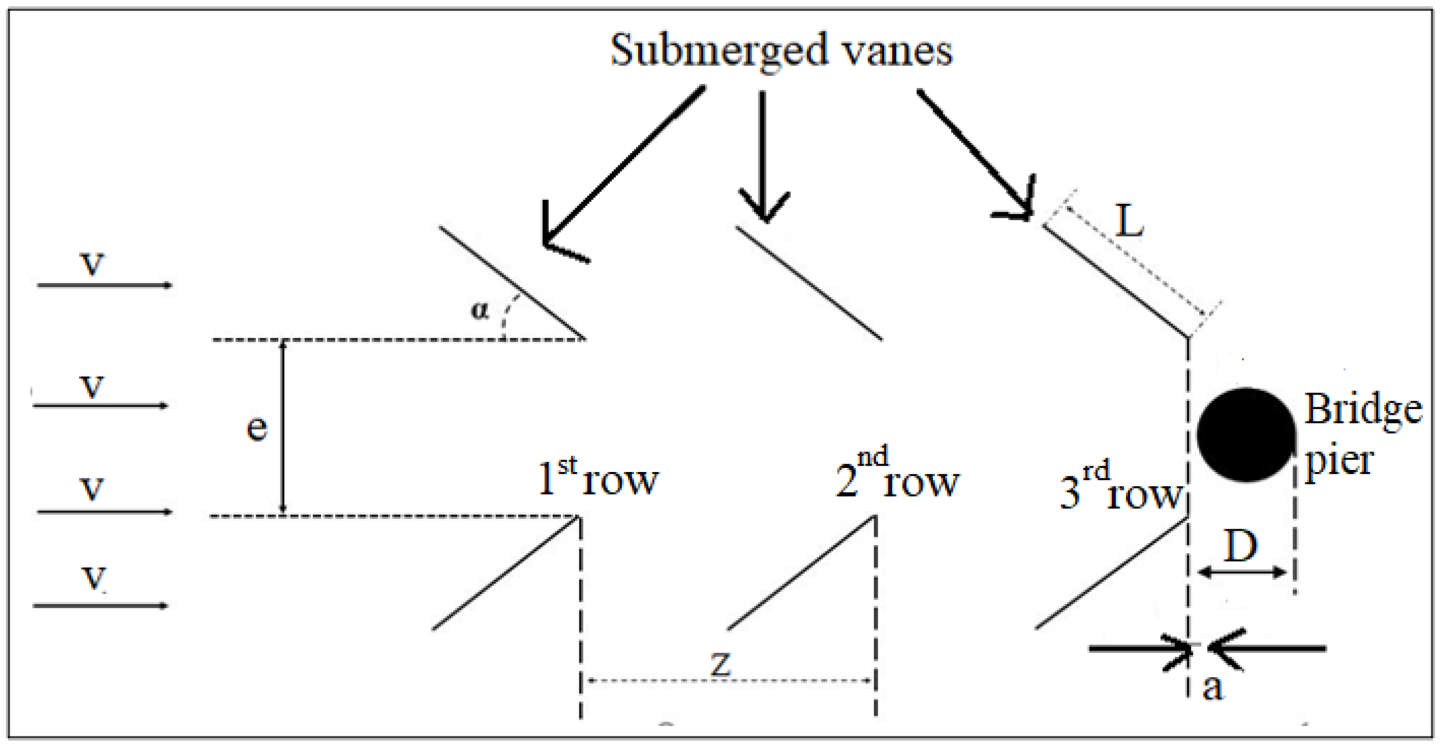
Figure 1. Schematic view of vanes installed.
Hydrology 12 00238 g001
Figure 2. Temporal variation in bed profile at pier location.
Hydrology 12 00238 g002
Figure 3. Flowchart of the GEP model.
Hydrology 12 00238 g003
Figure 4. Tree expression of the GEP (best individual shown as three sub–expression trees “Sub-ET 1–3”). Operators: − subtraction, + addition, ∗ multiplication, / division, Sqrt square root, 3Rt cube root, x2 squaring. Terminals: d 0 t / t e , d 1 α 1 , d 2 α 2 , d 3 α 3 , and c 0 is a learned constant.
Hydrology 12 00238 g004
Figure 5. Workflow of the ε –SVR used in this study.
Hydrology 12 00238 g005
Figure 6. Workflow of the feed-forward backpropagation ANN used in this study.
Hydrology 12 00238 g006
Figure 7. Area diagram of MLMs involved through the training and testing phases.
Hydrology 12 00238 g007
Figure 8. Scatter plot of MLM outcomes showing D s D versus measured values for training and testing phases. The 1:1 line is included for reference.
Hydrology 12 00238 g008
Figure 9. Distribution of DDR index for MLMs outcomes.
Hydrology 12 00238 g009
Figure 10. Taylor diagram of MLMs performance assessment.
Hydrology 12 00238 g010
Figure 11. Measured vs. predicted profile in location of bridge pier using GEP outcome.
Hydrology 12 00238 g011
Figure 12. Adaptability of observational and computational data of three models in the training and test steps.
Hydrology 12 00238 g012
Figure 13. (a) Residual distributions during training phase; (b) residual distributions during testing phase; (c) statistical indices (min, max, mean, total) of residuals for training; (d) statistical indices of residuals for testing.
Hydrology 12 00238 g013
Figure 14. Radar plot of MLMs’ outcomes for the training and testing stages.
Hydrology 12 00238 g014
Figure 15. Distribution of measured vs. predicted values of relative scour depth using MLMs involved.
Hydrology 12 00238 g015
Table 1. Summary of machine learning models applied for scour prediction.
ReferenceModels IncludedCase StudyFindings
[25]ANN, ANFIS, SVM, M5P, GEP, GMDHScour depth of bridge pierSVM performed better.
[26]Traditional empirical equations, RID, SVM, CAT, XGBScour depth at sluice outletXGB demonstrated superiority.
[27]SVR, RFR, Reptree, BRT, SGBScour depth of bridge pierSGB exhibited the highest performance.
[28]MLP, SVM, ANN, ANFISScour depth around group piersANN had the most accurate outcomes.
[29]Empirical models, BR, ABR, SVRScour depth of bridge pierAll MLMs outperformed empirical models.
[30]GEP, M5-TREE, MARS, ANFISScour depth of bridge pierNFIS model was the most superior.
[31]GA-ANNScour depth of bridge pierGA-ANN model predicted with high accuracy.
[32]AdaBoost, XGBoost, CatBoost, LightGBMScour depth of bridge pierXGBoost model outperformed others.
[33]ANFIS, GEPScour depth of bridge pierANFIS model was the most accurate.
[34]MGGPScour depth of bridge pierMGGP model had good prediction.
[35]SVM, ANFIS, GEPScour depth of bridge pierSVM had better outputs.
[36]MOSS, FBI, LSSVR, RBFNNScour depth of bridge pierMOSS exhibited fewer errors than others.
[37]GMDH, GMDH-HS, GMDH-SCEScour depth of complex bridge pierGMDH-SCE offered the best performance.
[38]GMDH, empirical equationsScour depth of bridge pier under wave conditionGMDH had less error.
[39]BPNN, RBFNN, SVMScour around monopile foundationsThe accurate model was the SVM.
[40]MLP, RBNN, empirical equationsScour depth in front of inclined bridge piersMLP and RBNN had more accuracy.
[41]ANNScour depth of bridge pierANN model was the superior.
[42]ANN-PSOScour depth of bridge pierHybrid model outperformed traditional methods.
[43]GEP, ANN, MNLRScour depth of bridge pierANN had better outputs.
[44]ANN, ANFIS, RMBed load transportData-driven techniques were well trained and tested.
[45]ANFISCoarse particle movement
Abbreviations: support vector machine (SVM); gene expression programming (GEP); artificial neural network (ANN); artificial neuro-fuzzy interface system (ANFIS); group method of data handling (GMDH); ridge regression (RID); cat boost (CAT); extreme gradient boosting (XGB); support vector regression (SVR); random forest regression (RFR); reduced error pruning tree (Reptree); bagging regression tree (BRT); stochastic gradient boosting (SGB); multi-layer perceptron (MLP); bagging regressor (BR); adaboost regressor (ABR); M5 model tree (M5-TREE); multivariate adaptive regression spline (MARS); genetic algorithm-based artificial neural network (GA-ANN); multigene genetic programming (MGGP); metaheuristics-optimized stacking system (MOSS); forensic-based investigation (FBI) algorithm; least squares support vector regression (LSSVR); radial basis function neural network (RBFNN); GMDH-harmony search algorithm (GMDH-HS); GMDH-shuffled complex evolution (GMDH-SCE); backpropagation neural networks (BPNNs); radial-basis neural network (RBNN); ANN–particle swarm optimization (ANN-PSO); multiple nonlinear regression analysis (MNLR); regression model (RM).
Table 2. The values of geometric properties involved.
Geometric DimensionNotationValueUnit
Number of vanesn2, 4, 6number
Collision angle of flow α 20–60degrees
Vane distance in flow directionz 1.5 D , 2 D cm
Vane distance perpendicular to flow directione D , 1.5 D , 2 D cm
Distance of the nearest vane to piera 0.5 D , 0 , 0.5 D cm
Length of vaneL9cm
Height of vaneH18, 27cm
Table 3. Typical SVR kernels (RBF used in this study).
KernelFunction
Linear K ( x i , x j ) = x i T x j
Polynomial K ( x i , x j ) = x i T x j + 1 d
Radial Basis Function (RBF) K ( x i , x j ) = exp γ x i x j 2
Sigmoid K ( x i , x j ) = tanh α x i T x j + c
Notation: K ( · , · ) is the kernel function; x i , x j R p are feature vectors; T transpose; d polynomial degree; γ > 0 RBF bandwidth; α , c sigmoid parameters; · Euclidean norm; tanh hyperbolic tangent.
Table 4. Summary of performance assessment metrics.
ModelPhaseRMSEMAE R 2 D s D DDR ( max )
SVMTraining0.22390.16920.78171.8964
Testing0.21410.17430.67222.2346
GEPTraining0.08640.06810.92374.2501
Testing0.07290.06410.91434.9405
ANNTraining0.15310.07940.73591.6720
Testing0.14760.08520.77212.1992
Table 5. Tuning parameters employed in the GEP model.
ParameterValue
Head size8
Number of chromosomes30
Number of genes3
Mutation rate0.044
Inversion rate0.1
One-point recombination rate0.3
Two-point recombination rate0.3
Gene recombination rate0.1
Gene transposition rate0.1
IS transposition rate0.1
RIS transposition rate0.1
Fitness function error typeRRSE
Linking function×
Disclaimer/Publisher’s Note: The statements, opinions and data contained in all publications are solely those of the individual author(s) and contributor(s) and not of MDPI and/or the editor(s). MDPI and/or the editor(s) disclaim responsibility for any injury to people or property resulting from any ideas, methods, instructions or products referred to in the content.