Improving Operational Ensemble Streamflow Forecasting with Conditional Bias-Penalized Post-Processing of Precipitation Forecast and Assimilation of Streamflow Data

Abstract

This work aims at improving the accuracy of ensemble streamflow forecasts at short-to-medium ranges with the conditional bias-penalized regression (CBPR)-aided Meteorological Ensemble Forecast Processor (MEFP) and streamflow data assimilation (DA). To assess the potential impact of the CBPR-aided MEFP and streamflow DA, or CBPR-DA, 20-yr hindcast experiments were carried out using the Global Ensemble Forecast System version 12 reforecast dataset for 46 locations in the service areas of 11 River Forecast Centers of the US NWS. The results show that, relative to the current practice of using the MEFP and no DA, or MEFP-NoDA, CBPR-DA improves the accuracy of ensemble forecasts of 3-day flow over lead times of 0 to 3 days by over 40% for 4 RFCs and by over 20% for 9 of the 11 RFCs. The margin of improvement is larger where the predictability of precipitation is larger and the hydrologic memory is stronger. As the lead time increases, the margin of improvement decreases but still exceeds 10% for the prediction of 14-day flow over lead times of 0 to 14 days for all but 3 RFCs.

1. Introduction

Since the launch of the Hydrologic Ensemble Forecast Service (HEFS) [1], the River Forecast Centers (RFC) in the US National Weather Service (NWS) have been producing ensemble streamflow forecasts for well over a decade. Similar ensemble streamflow forecast systems are used elsewhere with varying levels of complexity and operationalization [2]. With the national implementation of the HEFS completed for approximately 3000 forecast points, new efforts are underway to improve forecast accuracy, presenting new opportunities for advancing ensemble streamflow forecasting. As with single-valued streamflow forecasts, improving the accuracy of ensemble streamflow forecasts entails reducing input and hydrologic uncertainties such that the total uncertainty is minimized [3,4]. Input uncertainty may be differentiated into observed and future input uncertainties of which the latter is by far the larger. For this reason, input and future input uncertainties are used interchangeably in this paper unless a distinction is necessary. Hydrologic uncertainties include structural, parametric, initial condition (IC) and anthropogenic uncertainties, the last of which represents errors due to unknown or partially known human control or alterations of movement and storage of water, such as reservoir operations and diversions. Once the hydrologic models are selected and their parameters are specified, their state space is fully determined. Hence, structural or parametric uncertainty may not, in general, be addressed concurrently with the IC uncertainty.

There are two large contributing factors to input uncertainty. The first is biases in various statistical moments in the numerical weather prediction (NWP) forecasts, particularly in complex terrain. The second is scale mismatch between the NWP grids and the catchment size, the latter of which may easily span multiple orders of magnitude. To correct such biases in the NWP precipitation and temperature forecasts, the RFCs use the Meteorological Ensemble Forecast Processor [5,6,7,8] which inputs the ensemble mean precipitation and temperature forecasts from the Global Ensemble Forecast System (GEFS) [9]. Whereas the MEFP-generated precipitation ensembles are unbiased in the mean sense when all amounts of precipitation are considered, they tend to under-forecast heavy-to-extreme precipitation rather significantly [10,11]. Consequently, the resulting ensemble streamflow forecasts tend to be unconditionally unbiased but conditionally biased, which diminishes their utility and value for flood and inflow forecasting [12]. Recently, [13,14] have shown that the accuracy of the HEFS precipitation and streamflow forecasts for large events may be improved significantly with the conditional bias-penalized regression (CBPR)-aided MEFP. The improvement for large events, however, is achieved at the expense of reduced accuracy for small events resulting in marginally inferior unconditional performance compared to the operational MEFP.

To reduce hydrologic uncertainty, the Ensemble Post-Processor for streamflow (EnsPost) [4] was developed for the HEFS but not operationalized. A multi-scale post-processor for streamflow was also developed which was shown to significantly improve over EnsPost [15,16]. Post-processors, however, rely on static statistical relationships between the predictands and the predictors as inferred from large sample [17]. To address dynamically varying hydrologic uncertainties, such as the IC uncertainty, effectively, inverse problem-solving approaches, such as data assimilation (DA), which reflect the dynamics of the forward model used in forecasting, are generally necessary. Though referred to as streamflow DA for brevity, the data assimilated include not only streamflow but also precipitation, potential evapotranspiration and possibly others. DA, however, is yet to be implemented for the HEFS, though it was recognized as an integral component at inception [18].

The relative importance of input and hydrologic uncertainties and the relative effectiveness of reducing them vary greatly with predictability of precipitation and streamflow and its flow-dependent variations. For example, the residence time of surface runoff from saturation or infiltration excess is significantly shorter than that of subsurface runoff from soil storages [19]. Hence, reducing input uncertainty is often more important for forecasting high flows from large precipitation events whereas reducing the IC uncertainty is generally more effective for forecasting low-to-moderate flows owing to the longer memory in the subsurface runoff processes. Given this apparent complementarity between the CBPR-aided MEFP and streamflow DA in reducing total uncertainty, we postulate that a joint implementation of CBPR and DA is likely to improve the accuracy of streamflow forecasts not only for high flows but in the unconditional mean sense as well. The purpose of this work is to test the above postulate by assessing the impact of the CBPR-aided MEFP and streamflow DA for ensemble streamflow forecasting for short-to-medium ranges.

Streamflow DA addresses the IC uncertainty only. Hence, even if DA works ‘perfectly’, significant hydrologic uncertainty will generally remain. For this reason, the DA-aided ensemble streamflow predictions will still need to undergo post-processing to further improve accuracy as reflected in the design of the HEFS [1] (see Figure 1). Because DA tends to whiten errors in streamflow simulation particularly at short lead times, DA-aided ensemble streamflow forecasts may be post-processed in a simpler and potentially more parsimonious way, in which observed streamflow is no longer used as a predictor, than DA-less forecasts. Such a sequential operation of DA and post-processing (see Figure 1) would not only simplify statistical modeling of an ensemble streamflow forecast system but potentially reduce data requirements as well. A critical question for possible operationalization of the full HEFS [1] (see Figure 1) is then whether the joint performance of the CBPR-aided MEFP and streamflow DA is satisfactory for all ranges of flow as well as for high flows without the aid of streamflow post processing. To address the above, this work focuses on the evaluation of overall accuracy due to the CBPR-aided MEFP and streamflow DA as measured by the mean continuous ranked probability score (CRPS) [20]. We note here that post-processing of DA-aided predictions, including forecast attribute-specific verification [21], will be reported in the very near future in the context of component-specific contributions to predictive skill in the full HEFS depicted in Figure 1.

The main contribution of this work is the assessment of the likely impact of the joint implementation of the CBPR-aided MEFP and streamflow DA to the accuracy of the HEFS ensemble streamflow forecasts relative to operational practice. To this end, the impact of streamflow DA alone is also assessed. Effectiveness of streamflow DA varies with the length and strength of dynamically-varying hydrologic memory. This work advances understanding of the dependence of the effectiveness of streamflow DA on the streamflow generation processes that control hydrologic memory. The CBPR-aided MEFP is a statistical technique and hence its performance is susceptible to outlying hydrometeorological conditions. Streamflow DA is a dynamical technique but its performance depends on the fidelity of the hydrologic models. This work identifies hydrometeorological and hydrologic factors that may significantly impact the performance of the proposed approach. This paper is organized as follows. Section 2 describes the design of experiments and data, models and tools used. Section 3 describes the methods used. Section 4 presents the results and offers discussion. Section 5 provides the conclusions and future research recommendations.

2. Experiment Design, Data, Models and Tools Used

The study area comprises 46 headwater locations in the HEFS Testbed [13,22,23] in the service areas of 11 RFCs (see Figure 2 and Supplementary Materials Table S1). These locations are a subset of the study area used for the comparative evaluation of the CBPR-aided MEFP [13,14]. For brevity, the forecast points are identified by their five-character NWS abbreviations.

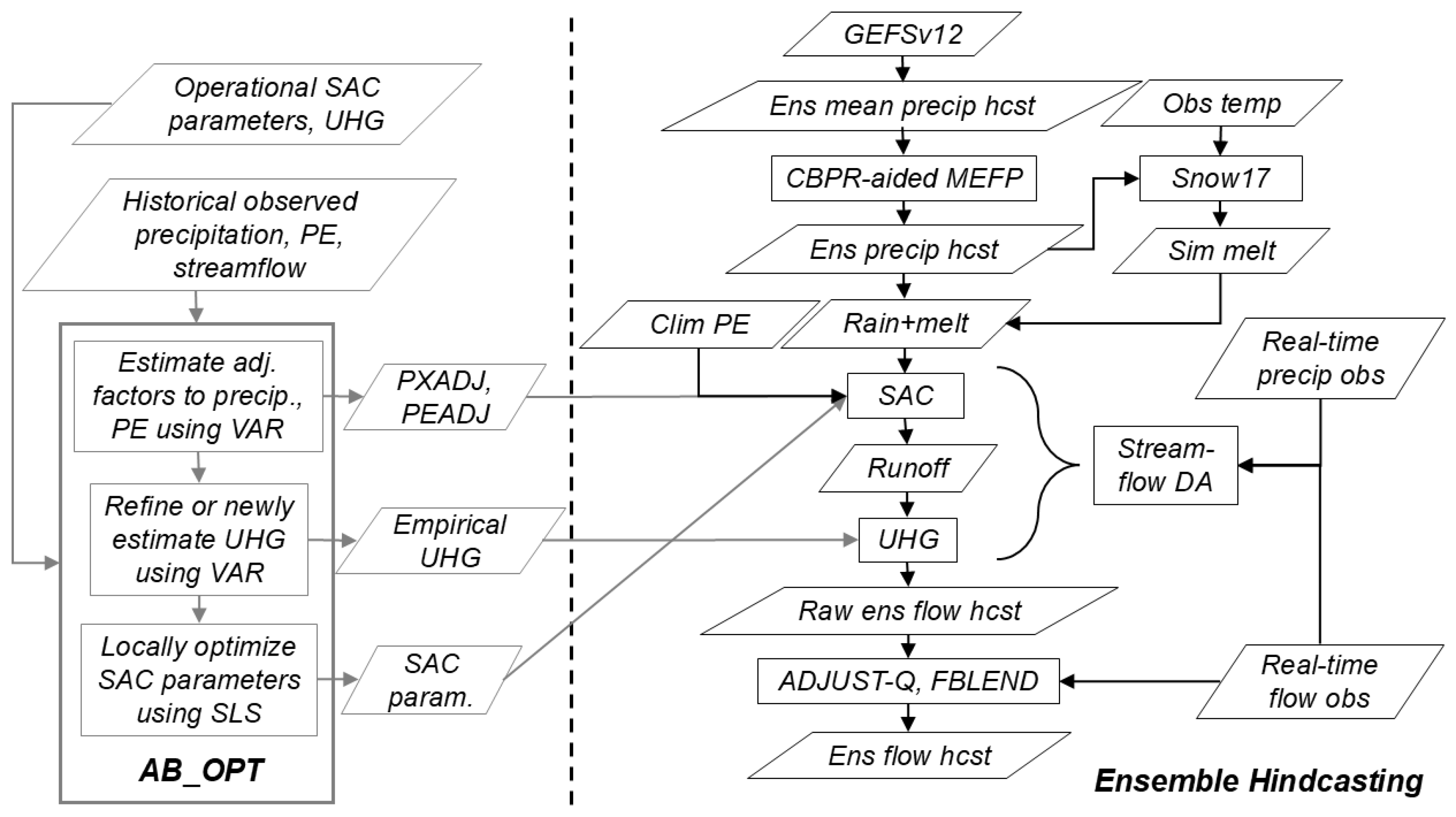
The ensemble precipitation hindcasts used are from the MEFP and the CBPR-aided MEFP forced by the GEFSv12 ensemble mean precipitation hindcasts [24,25] as used in [13,14]. The observed mean areal precipitation (MAP) data are from the RFCs. For both observed and future mean areal potential evapotranspiration (MAPE), climatological MAPE is used. The observed instantaneous streamflow data are from the US Geological Survey. The Community Hydrologic Prediction System (CHPS) [26] used by the RFCs for operational forecasting does not include automatic DA. To compare hindcasts with and without DA under identical conditions, it was therefore necessary to operate the hydrologic models outside of the CHPS following the RFCs’ operational configurations. The righthand side of Figure 3 shows the data flow and the operations used in the hindcast process with the CBPR-aided MEFP and streamflow DA. The hydrologic models used are the long-standing NWS operational models for headwater basins: Sacramento for soil moisture accounting (SAC) [27], Snow17 for snow ablation [28] and unit hydrograph for routing (UHG) [29].

Of the 46 locations, 9 in CN-, NW- and WGRFCs include multiple subbasins (see Supplementary Materials Table S1). Of the 7 NWRFC locations, glacier modeling is used for 2 locations but is neglected in this work. The glacier sub-basins help hold up late summer streamflows [31] but their contribution is relatively small. For those locations with snow modeling, we used simulated snowmelt instead of ensemble snowmelt forecasts based on ensemble mean areal temperature (MAT) forecasts. This simplification amounts to assuming clairvoyant MAT forecast by using observed MAT instead of forecast MAT and hence suppresses the future input uncertainty for temperature. Unlike the operational forecast process, the hindcast process has no real-time updating of snow water equivalent (SWE) [32]. Hence, it is very likely that the snowmelt simulation used in this work has considerably larger errors than that with SWE updating, and that the addition of future input uncertainty from forecast temperature would further complicate the assessment of the impact of the CBPR-aided MEFP and streamflow DA.

In Figure 3, ADJUST-Q and FBLEND, or A&F, refers to the long-standing interpolation–extrapolation procedure used at the RFCs to reconcile the difference between the observed and simulated flows valid at the forecast time and to extrapolate the difference (or ratio) to future timesteps (see Section 3.3 for details). Conceptually and mathematically, A&F is a form of streamflow post-processing; A&F weight-averages the latest observed flow and the raw forecast flow valid at some future timestep where the weight for the observed flow is made progressively smaller as the lead time increases. Though intended for single-valued forecasts, A&F may also be used as a poor man’s ensemble streamflow post-processor by applying it to individual members of the ensemble streamflow forecast. Unlike real post-processors, however, A&F has no ability to model uncertainty and hence cannot account for hydrologic uncertainty with fidelity. All hydrologic model parameters are based on the operational settings at the RFCs. The MARFC is transitioning from the continuous Antecedent Precipitation Index model to SAC [33]. Hence, their SAC parameter values used in this work are only preliminary. All models are run at a 6-h timestep in the hindcast process even though some RFCs use shorter timesteps for fast-responding basins. Because the collective information content in the observations varies greatly with the frequency of data ingest, the choice of the assimilation cycle has a large impact on DA performance. The use of a single fixed assimilation cycle is to facilitate the assessment of the impact of DA across different locations and regions.

Whether the timestep was changed or not, we used AB_OPT [30] (see the lefthand side of Figure 3) for all locations post factum to correct long-term biases in MAP and MAPE (PXADJ and PEADJ in Figure 3, respectively), refine the operational UHG (or newly estimate, if necessary) and locally optimize the SAC parameters using the operational settings as starting points. AB_OPT uses adjoint-based optimization, or variational assimilation (VAR), to estimate the biases and UHG and the sequential line search (SLS) [34] to refine the SAC parameters. The purpose of AB_OPT in this work is to reduce parametric and observed input uncertainties in model calibration as much as possible so that one may assess the performance of streamflow DA for its intended purpose of reducing the IC uncertainty as cleanly as possible. In the AB_OPT process, the period of record for historical MAP, MAPE and streamflow includes the hindcast period. Hence, AB_OPT already saw the events that occurred in the hindcast period and its results are used in hindcasting post factum.

3. Methods

This section describes CBPR used in the CBPR-aided MEFP [13,14] and adaptive conditional bias-penalized ensemble Kalman filter (AEnKF) [35,36,37] used for streamflow DA. The last subsection describes the approach used for comparative evaluation, operational considerations and limiting factors.

3.1. Conditional Bias-Penalized Regression

The main idea behind CBPR for the MEFP [13] is to trade accuracy for light precipitation in a measured way for improved accuracy for heavy-to-extreme precipitation. An example tradeoff point may be where one is willing to accept slightly increased unconditional root mean square error (RMSE) or mean continuous ranked probability score (CRPS) [20] in favor of significantly reduced conditional RMSE or mean CRPS for large events for single-valued and ensemble forecasts, respectively. CBPR exploits the fact that positive skewness in the predictands such as precipitation and streamflow tends to suppress and amplify the negative and positive impacts of such trades, respectively. An extremely appealing aspect of all such conditional bias (CB)-penalized approaches, including conditional bias-penalized kriging [38,39], multiple linear regression [12] and Kalman filter [36,37,40], is that the positive impact tends to be larger for larger events, with large implications for record-breaking events.

A variant of optimal linear estimation [41], CBPR may be viewed as a generalization of ordinary least-squares regression (OLSR). Assume that the forecast and observed precipitation are linearly related in standard normal space via:

$$W=\lambda Z+\epsilon$$

(1)

where $Z$ and $W$ are the forecast and observed precipitation in standard normal space following variable transformation, respectively, $\lambda$ is the CBPR coefficient and $\epsilon$ is a zero-mean normal random variable with which the conditional distribution of $W$ given $Z$ is also normal. By minimizing the linearly weighted sum of error variance and variance of Type-II error [42] with $\alpha$ as the weight for the latter, $J=E\left[{\left(\widehat{W}-W\right)}^2\right]+\alpha E[{\{E[\widehat{W}|W]-W\}}^2]$, one may obtain for $\lambda$ [13]:

$$\lambda ={\displaystyle \frac{(1+\alpha )\rho }{(1+\alpha {\rho }^2)}}, \alpha \ge 0, -1\le \rho \le 1,$$

(2)

where $\rho$ is the Pearson correlation between $Z$ and $W$ and $E\left[\widehat{W}|W\right]$ is prescribed via Bayesian optimal linear estimation [41] using Equation (1). For $\alpha =0$ (i.e., minimize error variance only), the CBPR solution reduces to the OLSR solution, i.e., $\lambda =\rho$. For $\alpha \to \infty$ (i.e., minimize the variance of Type-II error only), the CBPR solution reduces to the reverse regression solution, i.e., $\lambda =1/\rho$. The error variance of the CBPR prediction, $\widehat{W}=E\left[W|Z\right]= \lambda Z$, is given by ${\sigma }_{\widehat{W}}^2=E\left[{\left(\widehat{W}-W\right)}^2\right]={\lambda }^2-2\lambda \rho +1$ which, for nonzero $\alpha$, is always greater than error variance of the OLSR prediction, resulting in a larger uncertainty and hence larger ensemble spread. The CBPR parameter $\lambda$ is estimated via gradient-based cutoff-dependent minimization of conditional mean CRPS given a tolerable level of deterioration in unconditional mean CRPS and wet bias [13]. Depending on the premium that the user may place on improving the accuracy for large events vs. the aversion to reduced accuracy for small events, the tradeoff point may be varied [13]. In the CBPR-aided MEFP, CBPR is applied to a subset of the so-called canonical events [5]. For further details on the MEFP and the CBPR-aided MEFP, the reader is referred to [5,6,7,8,13].

3.2. Adaptive Conditional Bias-Penalized Kalman Filter

AEnKF is an ensemble version of the adaptive conditional bias-penalized Kalman filter (AKF) [35,36,37] which approximates for algorithmic simplicity and computational efficiency the conditional bias-penalized Kalman filter [40,43] and generalizes the Kalman filter (KF) [44]. The main idea behind AKF is to approximate the weighted sum of error variance and variance of Type-II error with an inflated error variance. AKF and AEnKF dynamically account for CB via a time-varying scaler weight, ${\alpha }_k$, as estimated based on the flow-dependent information content in the observations vs. model prediction. The implicit dependence of the weight on the (unknown) system states renders AEnKF effectively a nonlinear filter. Hence, if the time-varying weight can be prescribed accurately, AEnKF is superior to EnKF [45,46] not only in the tails of the predictand but also in the (unconditional) mean squared error sense. If the (positive) weight can only be prescribed statically, AEnKF is superior only in the tails and inferior near median resulting in a suboptimal filter. The AKF analysis solution, $X_{k|k}$, is given by [35,36,37]:

$$X_{k|k}=X_{k|k-1}+K_k[Z_k-H_k{X}_{k|k-1}]$$

(3)

where $X_{k|k-1}$ is the one step-ahead forecast state, $Z_k$ is the observation vector, $H_k$ is the observation structure matrix and $K_k$ is the AKF gain. The AKF gain, $K_k$, is given by:

$$K_k={\left(1+{\alpha }_k\right)\Sigma }_{k|k-1}{H}_k^T{[R_k+H_k{\left(1+{\alpha }_k\right)\Sigma }_{k|k-1}{H}_k^T]}^{-1}$$

(4)

where ${\Sigma }_{k|k-1}$ is the one step-ahead forecast covariance and $R_k$ is the observation error covariance. Note that Equations (3) and (4) are the same as the KF analysis and gain, respectively, except that the forecast error covariance is inflated by a factor of $\left(1+{\alpha }_k\right)$, ${\alpha }_k\ge 0$. AKF analysis error covariance, ${\Sigma }_{k|k}$, is given by:

$${\Sigma }_{k|k}={\Sigma }_{1+{\alpha }_k,k|k}{\Sigma }_{{(1+{\alpha }_k)}^2,k|k}^{-1}{\Sigma }_{1+{\alpha }_k,k|k}$$

(5)

where ${\Sigma }_{\beta ,k|k}$ denote the KF analysis error covariance in which forecast error covariance is inflated by a factor of $\beta$, $\beta \ge 1$. The inflated analysis error covariance, ${\Sigma }_{\beta ,k|k}$, is given by:

$${\Sigma }_{\beta ,k|k}{=\left[H_k^T{R}_k^{-1}{H}_k+{\left(\beta {\Sigma }_{k|k-1}\right)}^{-1}\right]}^{-1}=(I-K_k{H}_k)\beta {\Sigma }_{k|k-1}$$

(6)

In the above, the scaler weight, ${\alpha }_k$, is prescribed in each assimilation cycle by minimizing the information content for noise or, equivalently, maximizing the information content for signal [35,36,37,47]. The weight reflects the relative importance of CB or, equivalently, whether the true state of the system is near median or in the tails. If the state is near median (i.e., ${\alpha }_k=0$), AEnKF reduces to EnKF. If the state is in the tails (i.e., ${\alpha }_k\gg 0$), the model predictions from EnKF are over-confident due to lack of accounting of CB and AEnKF weighs observations more heavily than EnKF. If $\alpha \to \infty$, the model prediction has no information content and hence the AKF solution reduces to the static Fisher solution [41]. If streamflow is perfectly observed, under- or overconfidence in the model predictions is no longer relevant and the AEnKF and EnKF solutions converge. Streamflow at the outlet is arguably the single most informative representation of the state of the catchment. Hence, real-time streamflow observations allow reliable estimation of dynamically varying ${\alpha }_k$ even if significant observational uncertainties may exist. For this reason, AEnKF is particularly well suited for streamflow DA.

Depending on the formulation of the inverse problem, the number of uncertainty parameters employed in DA may vary significantly. To minimize the number of such parameters, we use an extremely parsimonious formulation which involves only eight true and one augmented state variables: the six SAC states valid at the beginning of the assimilation window, multiplicative biases for MAP and MAPE valid over the assimilation window and streamflow valid at the end of the assimilation window (i.e., forecast time) (see Figure 1 in [40]). The length of the assimilation window is set to the UHG duration. Though referred to as a filter, the above formulation amounts to a fixed-lag smoother [41] which explicitly captures the memory of the surface runoff processes. The above formulation is referred to in [36,37,40] as strongly constrained in that the hydrologic models are used as hard constraints under the assumption of no errors in the SAC soil moisture dynamics or in the SAC-generated runoff (i.e., Total Channel Inflow) which is input to UHG. A second motivation for the parsimony is to minimize the ensemble size for DA, and hence the amount of computation, and to keep the uncertainty modeling as simple as possible. In general, the larger the dimensionality of the state space is, the larger the ensemble size should be to attain comparable degrees of freedom in the inverse problem. Sensitivity analysis indicates that a relatively small ensemble size of 30 is acceptable for the above formulation. Depending on the RFC, the ensemble size for the precipitation hindcasts from the MEFP and CBPR-aided MEFP varies from 29 to 59, which is tied to the number of historical years available for the Schaake Shuffle [7,8]. With an ensemble size of 30 for DA, one may hence generate up to 870 to 1770 ensemble members which reflect both the future input and IC uncertainties. For streamflow forecast generation, one may substantially reduce the above ensemble size via subsampling with little loss of information content, depending on the follow-on processing steps in the forecast system.

Because estimation of ${\alpha }_k$ amounts to minimizing analysis error in real time, AEnKF does not require exhaustive calibration of uncertainty parameters, which is often subjective and expensive. Instead, the uncertain parameters are prescribed based on the knowledge of the observational uncertainties [48,49,50,51,52] and limited sensitivity analysis. The observational uncertainty models used in this work are:

$${\sigma }_P=0.25+0.39P$$

(7)

$${\sigma }_E=0.25+0.15E$$

(8)

and

$${\sigma }_Q=0.05+0.08Q$$

(9)

where $P$, $E$ and $Q$ are the 6-h MAP in $\mathrm{m}\mathrm{m}$, 6-h MAPE in $\mathrm{m}\mathrm{m}$ and instantaneous flow in ${\mathrm{m}}^3/\mathrm{s}$, respectively, and ${\sigma }_P$, ${\sigma }_E$ and ${\sigma }_Q$ are the associated standard deviation of observation error. The coefficients in Equations (7)–(9) are similar to those used in [35,37]. In reality, the above relationships likely vary from location to location as well as from event to event for precipitation. If additional information is available, one may refine the observational uncertainty models. Unlike homoscedastic uncertainty modeling [40], however, heteroscedastic modeling such as Equations (7)–(9) may limit uncertainty propagation through certain parts of the state space of the hydrologic models due to infeasible model dynamics. To avoid such a situation, it is a good practice to assess the sensitivity of the DA solutions to the uncertainty model parameters over the full dynamic ranges of the observations. For this reason, observational uncertainty models are generally not directly transferrable to different hydrologic models even if the inverse problem formulated and the DA technique used are the same. The limited sensitivity analysis indicates that AEnKF is much less sensitive to the coefficients in Equations (7)–(9) than EnKF and that the performance of AEnKF is very similar within a factor of 2 or so of variations in the coefficients. The DA formulation used in this work does not explicitly distinguish phase errors from amplitude errors. If significant timing errors exist, the quality of the DA solution is likely to deteriorate by varying degrees. Generally speaking, poor heteroscedastic uncertainty models or significant timing errors are less forgiving to strongly constrained DA. Such situations may be ameliorated by improving the observational uncertainty modeling or relaxing the strongly constrained formulation (see also Section 4.5).

3.3. Comparative Evaluation

A series of hindcast experiments was carried out in which CBPR or DA was included or excluded under otherwise identical conditions. In this way, we may assess the impact of the CBPR-aided MEFP and streamflow DA jointly as well as individually vs. the MEFP-forced streamflow hindcasts without DA. The latter represents the current RFC operations and hence serves as the baseline. Whereas the hindcast process largely follows the operational forecast process, there are two operational elements that could not be replicated in hindcasting: run-time modifications (MOD) and the operational forecast cycles. MODs are manual DA performed by human forecasters to keep the model states in line with the unfolding reality as inferred from real-time streamflow observations. MODs may include not only model states and input forcings but also model parameters, such as the UHG. For example, depending on where the rain may be falling relative to the catchment outlet, the forecaster may shift the UHG. It is possible to assess the impact of MODs using the RFC archive of operational forecasts [33]. Such an assessment, however, would be detached from the hindcast process in Figure 3 and hence was not considered in this work.

The second element of departure is that streamflow DA in the hindcast process is run every 6 h and DA-aided streamflow forecasts are generated every 24 h using the DA-updated model states valid at the same time as the input forecast. In this process, all observations and input forecasts are available every 6 and 24 h at all times without delay, respectively, and used immediately in streamflow forecast generation. In the RFC operations, however, ensemble streamflow forecasts are generated typically on a 24-h forecast cycle, which is generally different from the NWP cycles. Hence, the ingest of input forecasts for ensemble streamflow forecasting is usually delayed by 6 to 12 h [12]. In addition, real-time observations may be posting-delayed which would cut into lead time for MODs or post-processing. Hence, the baseline hindcast results seen in this work likely present a more favorable picture of forecast accuracy than may be attainable under the current RFC operational environment and practices.

Even if DA or MODs are not used, real-time streamflow observations may still be used in the DA-less forecast process via A&F which is a streamflow post-processor (see Section 2). The difference- and ratio-based A&F [53] is given by:

$$F_k=\left\{\begin{array}{c}{F}_k^r+{\displaystyle \frac{n-k}{n}}\left(O_0-F_k^r\right) if k\le n\\ F_k^r if k>n\end{array}\right.$$

(10)

and

$$F_k=\left\{\begin{array}{c}{F}_k^r{\left({\displaystyle \frac{O_0}{F_k^r}}\right)}^{\frac{n-k}{n}} if k\le n\\ F_k^r if k>n\end{array}\right.,$$

(11)

respectively, where $k$ is the lead time, $F_k$ is the $k$ timestep-ahead forecast from A&F, $F_k^r$ is the $k$ timestep-ahead raw (i.e., without A&F) forecast, $O_0$ is the latest observed flow valid at the prediction time (i.e., assuming no delay) and $n$ is the forecast horizon for blending. Note that Equation (10) is a linear weight-averaging operation in which the averaging forecast horizon is set by the location-specific parameter $n$. At the lead time of $0$, all weights are given to the observed flow whereas, at the lead timestep of $n$ and beyond, all weights are given to the raw forecasts. Equation (11) is a multiplicative version of Equation (10) in which the adjustment factor for the raw forecast is progressively varied between the lead times of $0$ and $n$. A set of heuristic rules is used to switch from Equation (11) to Equation (10) when Equation (11) is used to initiate A&F [53]. The A&F parameter $n$ should preferably be prescribed location-specifically based on flow-dependent optimization. At the RFCs, however, $n$ is set to a fixed value heuristically which is followed in this work. Because both A&F and DA use observed flow, comparing DA-less hindcasts with A&F and DA-aided hindcasts without A&F may appear straightforward. There exists, however, a rather important consideration before such a comparison may be made as explained below.

Whereas A&F does not consider uncertainty and hence assumes that streamflow is perfectly observed, DA explicitly considers observational uncertainties. When the DA-aided hindcasts are verified, however, it is almost always assumed for simplicity that the verifying streamflow observations are perfect [54]. A consequence of the above inconsistency is that, whereas the A&F-aided hindcast perfectly matches the observed flow at prediction time (i.e., $k=0$ in Equations (10) and (11)), the DA-aided does not, thereby being penalized for being uncertainty-aware. To allow comparative evaluation while following the RFCs’ operational practices, we apply A&E to all ensemble hindcasts using the RFC parameters but with the observed flow replaced with the perturbed observed flows used in AEnKF, i.e., the ensemble traces of $Z_k$ in Equation (3) where the perturbations come from Equation (9). Because the observational uncertainty for streamflow used in this work is relatively small, the above substitution in A&F has negligible impact on DA-less hindcasts. For DA-aided hindcasts, the use of A&F as described above amounts to applying poor man’s streamflow post-processing with ill-prescribed parameters which may compromise the hindcast quality particularly at short lead times. Hence, the use of the A&E for the DA-aided hindcasts is solely to mimic the operational forecast process for comparison, rather than to improve accuracy. In the full HEFS, ensemble streamflow post-processing would follow DA as shown in Figure 1 to further improve accuracy.

4. Results and Discussion

This first three subsections present the results from the comparative evaluation of (1) MEFP-DA vs. MEFP-NoDA, which assesses the impact of DA when the MEFP ensemble precipitation hindcasts are used as the common input for future precipitation, (2) CBPR-NoDA vs. MEFP-NoDA, which assesses the impact of CBPR without DA, and (3) CBPR-DA vs. MEFP-NoDA, which assesses the joint impact of CBPR and DA. Section 4 presents the results of CBPR-DA vs. MEFP-NoDA based on the operational SAC parameters (including PXADJ and PEADJ) and UHG with no refinement, i.e., without the post-factum reduction of hydrologic uncertainties in model calibration via AB_OPT. In the above, CBPR and DA refers to the CBPR-aided MEFP and streamflow DA, respectively. The hindcast period is from 2000 to 2019. The primary performance measures used are mean CRPS and CRPS skill score (CRPSS). Assessment of CBPR and AEnKF in terms of specific forecast attributes such as reliability, resolution and discrimination [42] has been reported in [13,40] and is not addressed in this paper.

4.1. Impact of DA

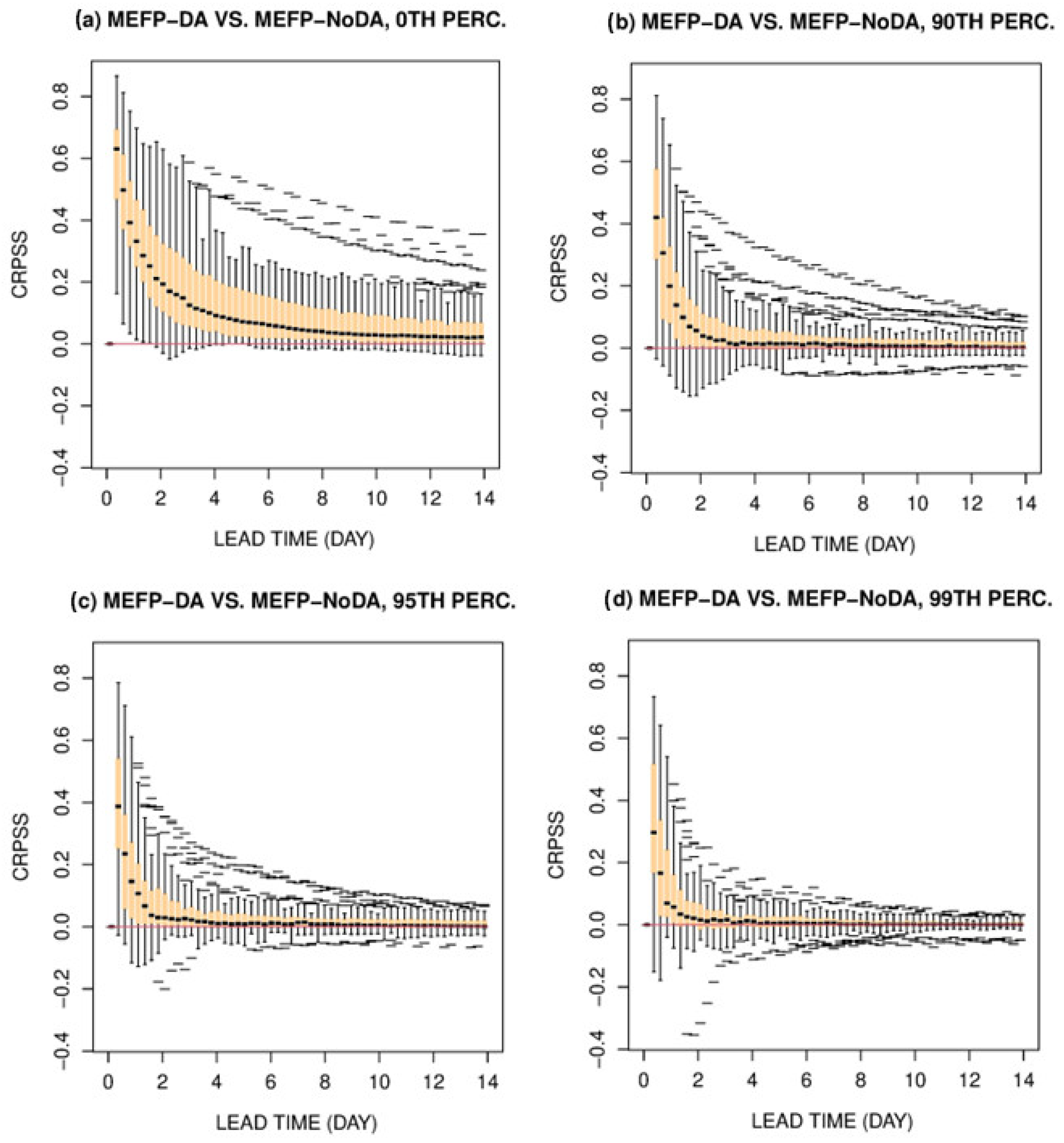
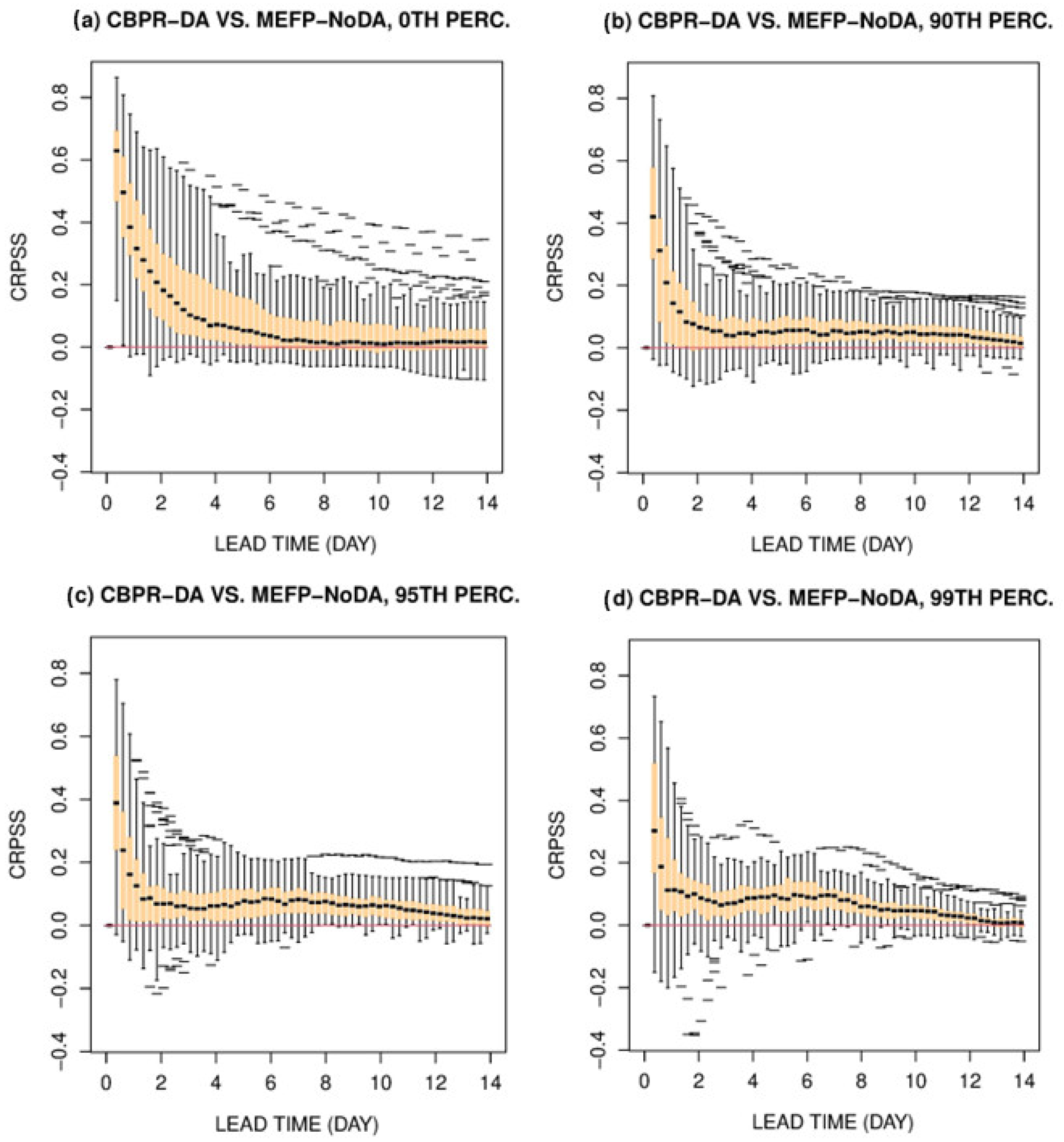
Figure 4 shows the CRPSS of MEFP-DA in reference to MEFP-NoDA as a function of lead time where the CRPSS is defined as:

$$CRPSS={\displaystyle \frac{{\overline{CRPS}}_{MEFP-NoDA}-{\overline{CRPS}}_{MEFP-DA}}{{\overline{CRPS}}_{MEFP-NoDA}}}=1-{\displaystyle \frac{{\overline{CRPS}}_{MEFP-DA}}{{\overline{CRPS}}_{MEFP-NoDA}}}$$

(12)

where ${\overline{CRPS}}_{MEFP-NoDA}$ and ${\overline{CRPS}}_{MEFP-DA}$ are the mean CRPS of MEFP-NoDA and MEFP-DA, respectively. Figure 4a shows the unconditional CRPSS which reflects all hindcasts for all ranges of verifying observed flow. Figure 4b–d show the conditional CRPSS which reflects only those hindcasts for which the verifying observed flow exceeds the 90th, 95th and 99th percentiles, respectively. Note that the conditional CRPSS is not a proper score and hence may be gamed [55,56]. If used by itself, such a score will frequently lead to poor decisions as high flows occur infrequently. Potential for misinterpretation or misuse of such conditional verification information may be minimized by accompanying it with the unconditional verification information and the relationship between the two. For example, for mean $CRPS$, one may write:

$$E\left[CRPS\right]=E\left[CRPS|obs>q_c\right]\mathrm{Pr}\left[obs>q_c\right]+E\left[CRPS|obs\le q_c\right]\mathrm{Pr}\left[obs\le q_c\right]$$

(13)

where $obs$ is the observed flow, $q_c$ is the threshold flow of choice and $\mathrm{P}\mathrm{r}[·]$ is the probability of occurrence of the event bracketed. Note in Equation (13) that $\mathrm{Pr}\left[obs>q_c\right]$ is the familiar exceedance probability. One may use any conditioning event of one’s interest as long as the two conditioning events in Equation (13) are mutually exclusive and collectively exhaustive.

Figure 4 shows the CRPSS results of MEFP-DA in reference to MEFP-NoDA in the form of box-and-whisker plots vs. lead time. Supplementary Materials Figure S1 provides line-plot renditions of the same results which show the location-specific patterns of CRPSS vs. lead time. In each box-and-whisker plot, there are 46 data points, each representing a location (see Figure 2 and Supplementary Materials Table S1). The midline in the box is the median. The upper and lower ends of the box are the 75th and 25th percentiles, respectively. The whiskers represent 1.5 times the interquartile range from the top and bottom of the box to the largest and smallest data points within that distance, respectively. Any outlying data points are identified individually. The average sample size for each location for the unconditional results is 5758. Those for the conditional results are 558, 274 and 54 for the 90th, 95th and 99th percentiles, respectively. The saw-tooth patterns for certain locations seen in the CRPSS line plots (see Supplementary Materials Figure S1) are due to diurnal variations in the skill of the input hindcasts [12]. Note in Figure 4 that the CRPSS values at lead time of zero, i.e., the skill for the analysis, are very close to zero due to the fact that A&F was applied to all hindcasts, rendering all analyses to closely match the observed flow as explained in Section 3.3. The large CRPSS values at short lead times beyond zero reflect the large skill in the DA-aided hindcasts and the rather small $n$ values used in A&F at the RFCs for a number of locations. The above observation suggests that the performance of A&F may improve potentially significantly via location-specific flow-dependent optimization of $n$.

Figure 4a may be summarized as follows. Streamflow DA consistently improves the accuracy of ensemble streamflow hindcasts in the unconditional mean sense for all locations across almost all lead times considered. The improvement is larger for shorter lead times. The margin of improvement varies significantly from region to region and from location to location (see Supplementary Materials Figure S1) in reflection of the variations in hydrologic memory and predictability of precipitation. Figure 4b–d may be summarized as follows. The larger the verifying observed flow is, the smaller the margin of improvement by streamflow DA is and the more quickly the improvement dissipates as the lead time increases. For a small number of locations, streamflow DA performs poorly up to a few days of lead time. At the highest conditioning level of 99th percentile flow, streamflow DA adds significant positive skill up to 2 days of lead time and small but positive skill out to Day 14 for most locations. The two locations in CNRFC with slightly negative CRPSS beyond Day 5 (see Supplementary Materials Figure S1) are FTJC1 and NFDC1, both of which include snow modeling. The likely cause for the above is that snowmelt simulation may have large errors which, without SWE updating, would be incorrectly attributed by streamflow DA. Overall, Figure 4 is in agreement with the flow-dependent variations in hydrologic memory posited in Section 1.

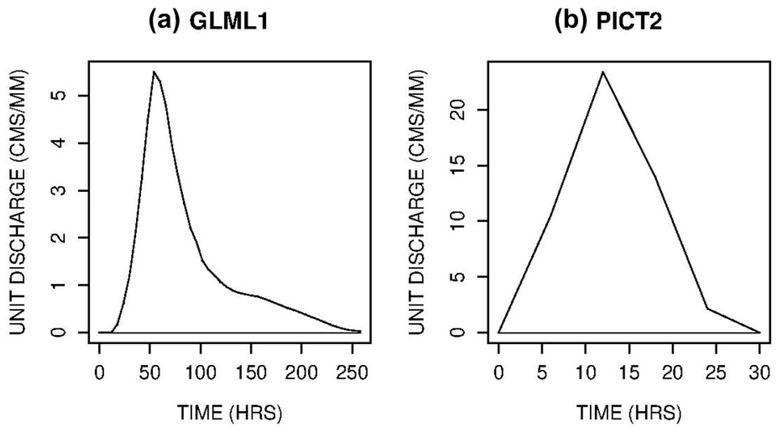
We now turn our attention to the small number of locations in Figure 4b–d (see also Supplemental Materials Figure S1) for which CRPSS values are significantly negative over different stretches of lead time. Streamflow DA used in this work does not distinguish phase errors from amplitude errors (see Section 3.3). Hence, if the simulated flow leads or trails the observed, DA is likely to over- and under-react, respectively, resulting in out-of-phase forecast hydrographs. The two locations with the largest negative CRPSS values in Figure 4d (see also Supplementary Materials Figure S1) are PICT2 in WGRFC and GLML1 in LMRFC. To identify possible sources of such errors, it is instructive to examine the hydrologic attributes of the catchments (see Figure 2 and Supplementary Materials Table S1) and their UHGs (see Figure 5).

GLML1 is a 1292 km² headwater basin for the Calcasieu River which drains into the Gulf of Mexico. GLML1 is extremely flat with a channel slope of only about 0.07%. Even if runoff is estimated very accurately, routing in such a catchment is subject to very large uncertainties due to the large degrees of freedom in flow paths. Figure 5a shows the 6-h UHG for GLML1 used in this work which shows an extremely large time-to-peak of over 2 days. Figure 5a represents a least-squares solution based on the MAP and streamflow data that include all events within the 20-yr hindcast period. Given the physiography of the catchment, it is very likely that event-specific UHGs vary significantly and, depending on the event, the actual hydrograph response may differ considerably from Figure 5a resulting in timing errors of varying magnitude and direction. PICT2 is a 1178 km² basin located in semi-arid central Texas and has an elongated shape with a stream length of 117 km. Streamflow response is generally flashy as runoff occurs primarily via infiltration excess from convective rainfall which may cover only parts of the catchment. Hence, the UHG assumptions are often not met. Figure 5b shows that the UHG at 6-h timestep used in this work is too coarse to resolve the hydrograph response. Examination of the 1-h UHG (see Figure B1 in [30]) indicates that the time-to-peak at the outlet is only about 6 h and that, depending on the rain area relative to the catchment outlet, the actual hydrograph response may differ considerably due to the significant differences in travel time.

Figure 6 shows the mean CRPS of MEFP-NoDA (black), MEFP-DA (blue) and CBPR-DA (red) for PICT2 and GLML1. The extreme flashiness of PICT2 is readily seen in Figure 6b. In Figure 6, MEFP-DA and CBPR-DA overlap over short lead times and hence only MEFP-DA is visible. Over the lead times that correspond to the time-to-peak of the UHG at the respective locations, the DA-aided forecasts are less accurate than MEFP-NoDA due to the premature or belated correction of the state variables arising from timing errors. Because out-of-phase errors tend to occur over lead times where hydrologic uncertainty dominates over input uncertainty, CBPR-DA does not improve accuracy until hydrologic memory dissipates at longer lead times. The CRPSS results for CBPR-DA in reference to CBPR-NoDA are very similar to Figure 4. This similarity is an indication that the impact of streamflow DA is similarly positive whether the precipitation forecasts come from the MEFP or the CBPR-aided MEFP. This picture, however, is likely to change if the quality of the precipitation forecasts differs greatly.

4.2. Impact of CBPR

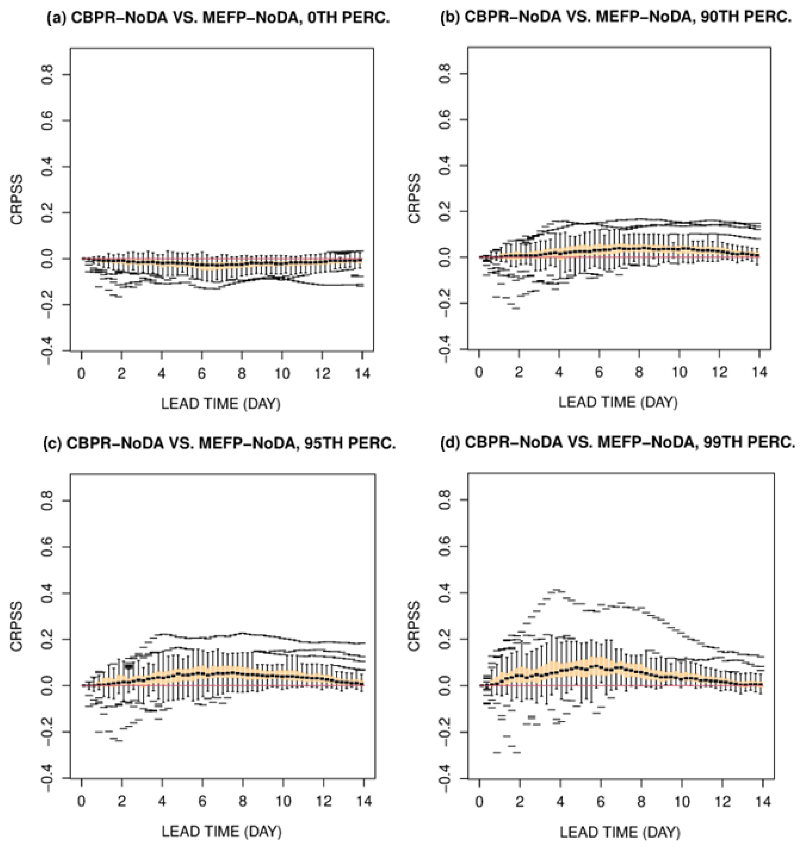
Figure 7 shows the CRPSS of CBPR-NoDA in reference to MEFP-NoDA. The figure hence assesses the impact of the CBPR-aided MEFP vs. the MEFP currently in operation. Supplementary Materials Figure S1 provides line-plot renditions of the same results which show the location-specific patterns of CRPSS vs. lead time. Figure 7 may be summarized as follows. In general, CBPR improves the hindcasts for large flows and the margin of improvement is larger for larger flows. In the unconditional mean sense, however, CBPR deteriorates the hindcasts due to the tradeoff explained in Section 3.1. There are a few locations where the deterioration by CBPR is rather significant (see Supplementary Materials Figure S1). By far the most conspicuous are SESC1 and UKAC1 in CNRFC and, to a lesser degree, PYAV2 in MARFC. The above three locations are responsible for most of the negative CRPSS values seen in Figure 7b–d.

The cause for the deterioration for SESC1 is traced to the poor quality of the CBPR-aided MEFP hindcasts at this location [13,14]. At SESC1 and, to a lesser degree, UKAC1, the ensemble mean hindcasts have extremely large heteroscedastic errors, forming bifurcating upper tails vs. verifying observations. Such errors occur due to the atmospheric flow-dependent variations in predictability and predictive skill of precipitation in the region [57]. The CBPR coefficient $\lambda$ (see Equation (2)) is optimized by minimizing conditional mean CRPS in which the conditioning threshold is increased incrementally until one of the two acceptance criteria for tradeoff is violated [13]. Such magnitude-dependent estimation of $\lambda$ is necessarily more susceptible to magnitude-dependent heteroscedastic errors than OLSR which always uses all available pairs of forecast and observation in the bivariate normal space. PYAV2 has a drainage area of 1716 km in the Blue Ridge Mountains with two main tributaries running in perpendicular directions. The 6-h UHG indicates a time-to-peak of approximately 18 to 24 h. Visual examination of the simulated vs. the observed hydrographs indicates significant timing errors for large events at this location. For example, the timing error for the largest observed peak is about 18 h which is almost as large as the time-to-peak. Such large timing errors are likely to deteriorate DA performance over a wide stretch of the forecast horizon as seen in Figure 7. Figure 7b–d also show that the improvement by CBPR for large conditioning thresholds tends to be larger for the SERFC locations (see Supplementary Materials Figure S1). A significant contributing factor to the above is that the operational MEFP at SERFC has large room for improvement in the selection of the canonical events and modeling of the probability distributions of observed and forecast precipitation amounts. The improvement by the CBPR-aided MEFP over the operational MEFP for high flows reflects the improvement in the above as well.

4.3. Impact of CBPR and DA

Figure 8 shows the CRPSS of CBPR-DA in reference to MEFP-NoDA and hence assesses the joint impact of CBPR and streamflow DA vs. the baseline representing the current RFC operation. Supplementary Materials Figure S1 provides line-plot renditions of the same results which show the location-specific patterns of CRPSS vs. lead time. Compared to Figure 4a, Figure 8a shows that the margin of improvement by CBPR-DA over MEFP-NoDA is not as large as that of MEFP-DA over MEFP-NoDA. This is due to the fact that CBPR deteriorates the accuracy of the MEFP precipitation hindcasts in the unconditional mean sense. There are some locations in Figure 8a for which the CRPSS values are negative over different stretches of lead time (see also Supplementary Materials Figure S1). At such locations, conditional performance for large events tends to improve as may be expected from the tradeoff described in Section 3. Figure 8a shows that, whereas CBPR-DA is marginally inferior to MEFP-DA in the unconditional mean sense, it greatly improves unconditional performance over MEFP-NoDA.

Sample size for the 99th percentile results is relatively small. To assess sampling uncertainty for Figure 8d, confidence intervals were calculated for each location via bootstrapping (see Supplementary Materials Figure S2). The 98% confidence intervals indicate that the positive CRPSS results for the 99th percentile threshold are generally statistically significant. The confidence intervals also accentuate the DA challenges for those locations identified above as having large hydrologic or input uncertainty. Comparison of Figure 8b–d with Figure 4b–d may be summarized as follows. CBPR-DA does not, in general, improve conditional performance over MEFP-DA over short lead times where hydrologic memory dominates. Over longer lead times where input uncertainty is more important; however, CBPR-DA significantly improves conditional performance over MEFP-DA.

The above transition occurs at approximately Days 4, 2 and 1 for the conditioning thresholds of 90th, 95th and 99th percentiles, respectively, in reflection of the increasingly shorter hydrologic memory for larger events. Compared to MEFP-NoDA, CBPR-DA not only improves conditional performance greatly over short lead times owing to the strong hydrologic memory exploited by streamflow DA effectively but also improves conditional performance significantly over longer lead times owing to the improved precipitation hindcasts by CBPR for large events. There are, however, a number of locations for which the conditional performance of CBPR-DA is inferior to that of MEFP-NoDA particularly at the 99th percentile threshold. Though difficult to discern individual curves due to sampling noise (see Supplementary Materials Figure S1), the noticeably negative CRPSS values are associated with FTJC1 and SESC1 in CNRFC, GLML1 in LMRFC, PYAV2 in MARFC, SPEW1 and SRMO1 in NWRFC and PICT2 in WGRFC. Of these locations, by far the most negative values are associated with GLML1 and SESC1. The probable causes for negative CRPSS for GLML1, SESC1, PICT2 and PYAV2 are already described in Section 4.1 and Section 4.2. Of the above locations, FTJC1, SPEW1 and SRMO1 include snow modeling and hence they are more susceptible to over- or under-correction by DA due to incorrect attribution of errors as explained in Section 4.1. Figure 8 indicates that, overall, CBPR-DA improves over MEFP-NoDA both conditionally and unconditionally as postulated in Section 1.

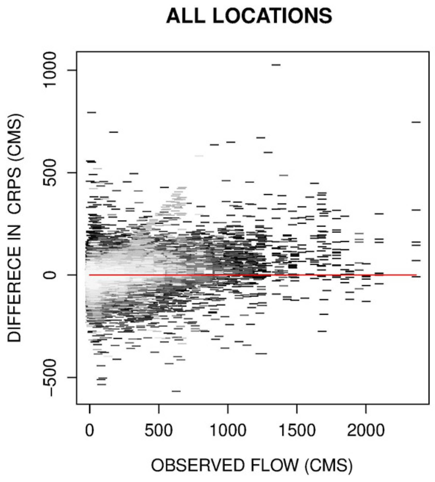
The practical significance of the improvement by CBPR-DA over MEFP-NoDA across all locations may be seen plainly in a single plot of $∆CRPS={CRPS}_{MEFP-NoDA}-{CRPS}_{CBPR-DA}$ vs. verifying observed flow. A positive $∆CRPS$ indicates improvement by CBPR-DA over MEFP-NoDA and a larger $∆CRPS$ indicates a larger improvement. Figure 9 shows $∆CRPS$ vs. verifying observation between the lead times of 0 and 7 days for all 46 locations. The figure has over 7.7 million data points of $∆CRPS$, each representing a matching pair of CBPR-DA and MEFP-NoDA hindcasts vs. the common verifying observed flow. The data points for the same location share the same gray scale which varies from black to light gray according to the dynamic range of the observed flow (the larger, the darker). Hence, one may gauge how $∆CRPS$ may vary with verifying observed flow across different locations. Because the CRPS of a single-valued forecast is its absolute error (AE), the CRPS of an ensemble forecast is closely related to the AE of its ensemble mean forecast. Hence, the difference in AE between the MEFP-NoDA and MEFP-DA ensemble mean forecasts is similar to Figure 9 but more dispersive in the vertical due to the perfect sharpness of the ensemble mean forecasts. Figure 9 is hence indicative of the potential impact of CBPR-DA across the dynamic range of observed flow both in the ensemble sense and in the ensemble mean sense. It is readily seen in Figure 9 that CBPR-DA outperforms MEFP-NoDA by significant margins over a wide range of significant to large verifying observed flow, and that the large improvement in unconditional performance seen Figure 8a is due to this wide-ranging outperformance.

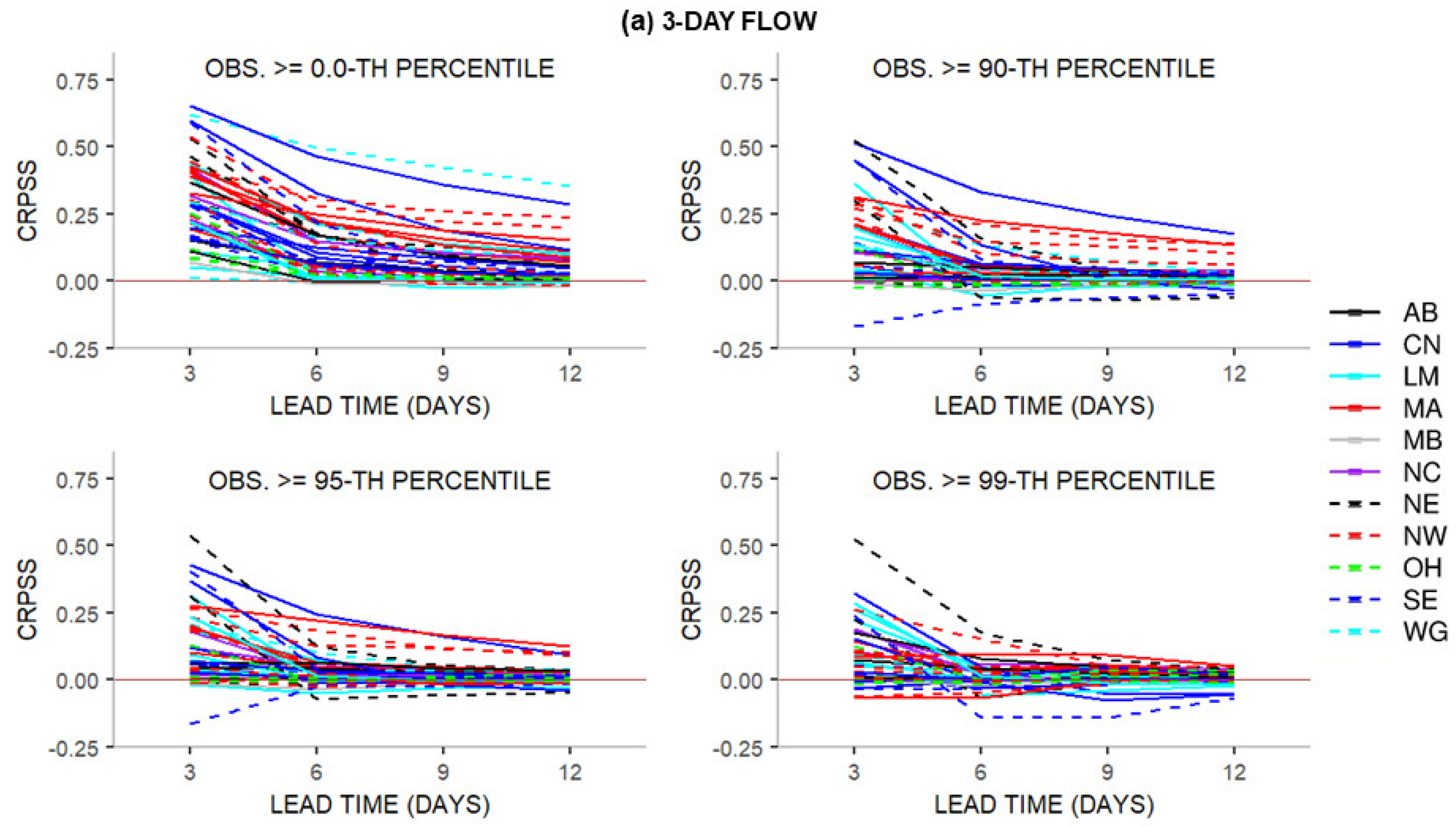
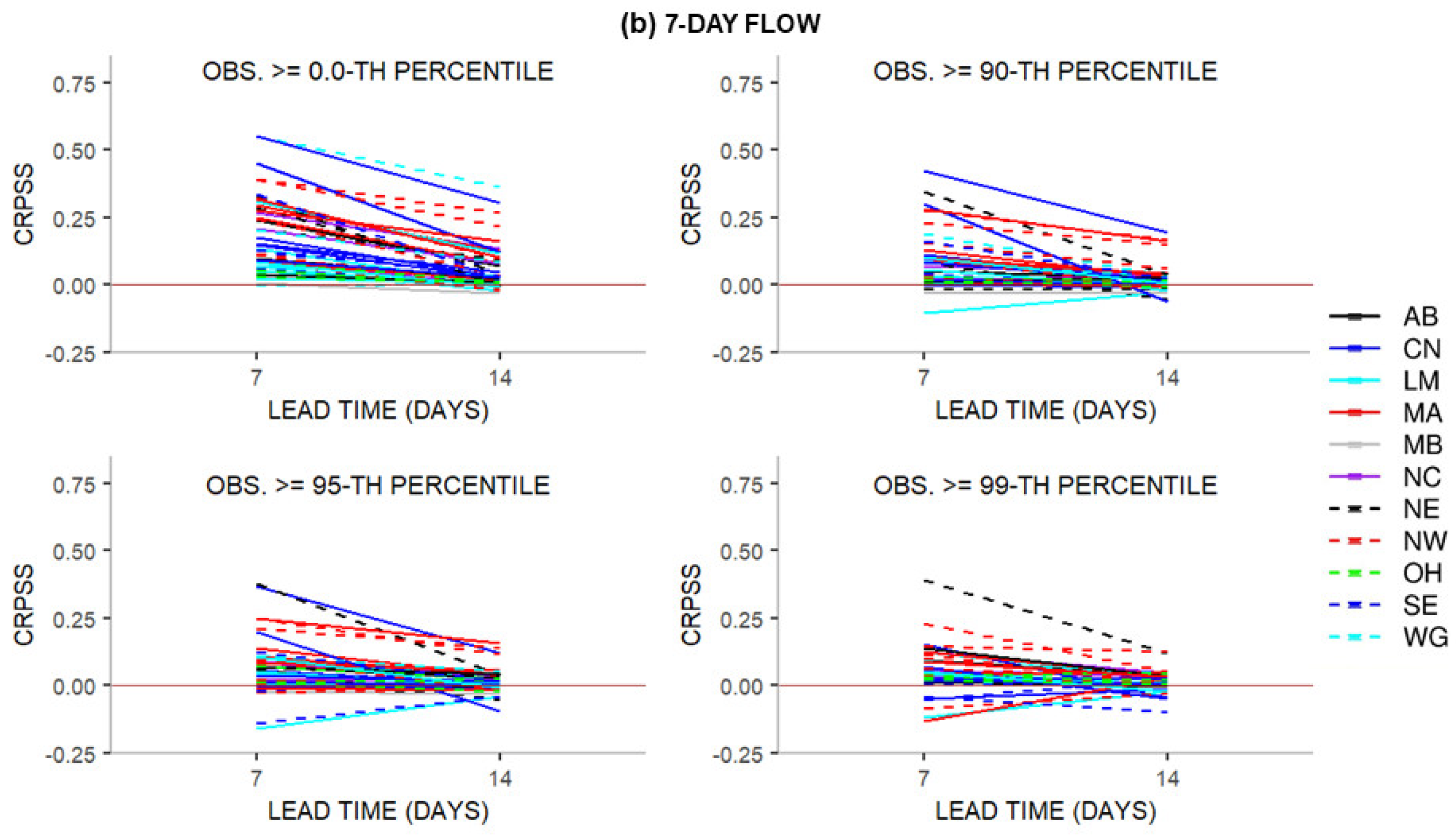
The results presented above are for predictions of instantaneous flow at 6-h timestep. In many applications such as reservoir operations, forecasts of multi-daily flows are of particular interest. Figure 10a,b show the CRPSS of CBPR-DA for mean 3- and 7-day flows in reference to MEFP-NoDA, respectively. The left-most panels show the unconditional CRPSS. The rest of the panels show CRPSS conditional on verifying observed flow exceeding the 90th, 95th and 99th percentiles. All multi-daily flows mentioned in this paper are mean flows averaged over the respective aggregation periods. Figure 10 is qualitatively similar to Figure 8 and shows that CBPR-DA improves prediction of multi-daily flows over MEFP-NoDA unconditionally for all locations and conditionally for most locations for all thresholds, and that the margin of improvement varies greatly from region to region and from location to location depending on the predictability of precipitation [13] and hydrologic memory [16]. Expectedly, the relative performance of CBPR-DA diminishes as the conditioning threshold increases and the aggregation period increases.

4.4. Impact Without Post-Factum Reduction of Hydrologic Uncertainty in Model Calibration

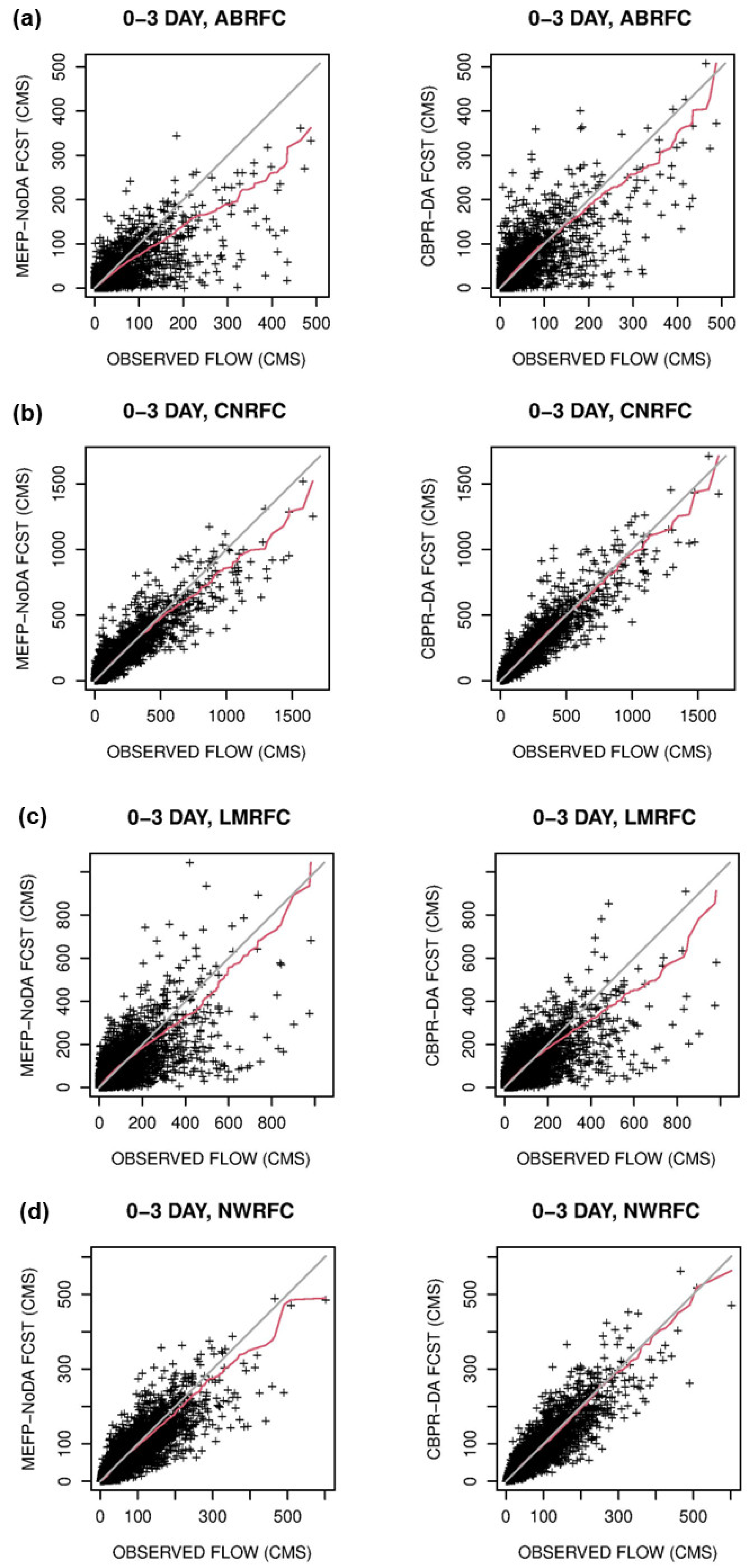
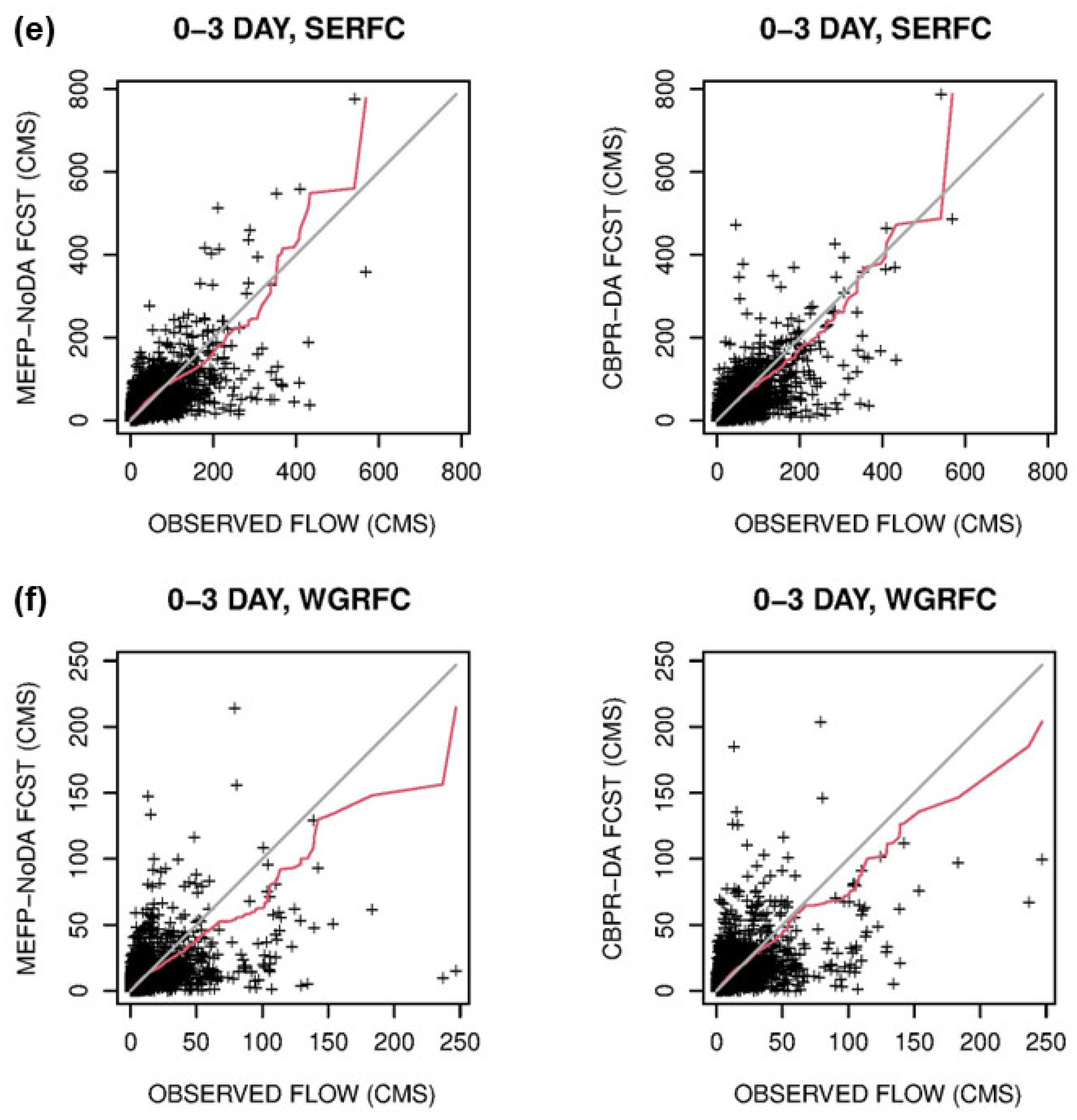
All results presented above are based on the post-factum correction of long-term biases in MAP and MAPE, refinement of UHG and local optimization of the SAC parameters using AB_OPT and SLS to minimize observed input and parametric uncertainties (see Figure 3). In the real world, however, the observed forcings may have significant biases or the hydrologic model parameters may be of questionable quality due, e.g., to lack of data particularly for large events. To assess the impact of CBPR-DA under more realistic conditions, we repeated the hindcast experiments without applying AB_OPT except to newly estimate empirical UHGs for 10 locations at a 6-h timestep. For the above 10 locations, the RFCs operate SAC-UHG at timesteps smaller than 6 h and hence 6-h operational UHGs are not available (see Supplementary Materials Table S1). Thus, the results in this subsection are based largely on the operationally used SAC parameters (including PXADJ and PEADJ) and UHG, and hence more indicative of the potential impact of operationalizing the CBPR-aided MEFP and streamflow DA. Figure 11 shows the resulting scatter and quantile-quantile (Q-Q) plots of the MEFP-NoDA (left panels) and CBPR-DA (right panels) ensemble mean hindcasts for mean 3-day flow over lead times of 0 to 3 days vs. verifying observed flow for 6 RFCs. Ensemble mean forecasts linearly reflect all ensemble members and hence are sensitive to outlying members while preserving mass in the mean sense. In addition, being perfectly sharp, ensemble mean forecasts do not hedge. For these reasons, critical examination of ensemble mean forecasts is an extremely useful additional check on the quality of ensemble precipitation or streamflow forecasts. The study locations used for each RFC are very limited in number and hence may not be representative of the entire service area of the RFC. For the purpose of summarizing the results, however, we collectively refer to the study locations by their RFC name.

In Figure 11, the tighter the scatter is around the one-to-one line, the more accurate the ensemble mean prediction is. The closer the Q-Q plot is to the one-to-one line, the more similar the marginal distribution of the ensemble mean prediction is to that of the verifying observation. Q-Q plots indicate how closely the predictions bunch up or spread out over different subranges of the predictand vs. the verifying observation with no regard to data point-specific association. Hence, one may qualitatively assess the severity of conditional bias by jointly examining scatter and Q-Q plots over different subranges of the verifying observation [40]. The following observations may be made in Figure 11 and similar plots for all other RFCs. The accuracy of MEFP-NoDA varies greatly from RFC to RFC in reflection of the regional variations in predictability of precipitation and streamflow. For a number of RFCs, CBPR-DA substantially improves over MEFP-NoDA and significantly reduces severe under-forecasting of large flows. For RFCs with large predictability, CBPR-DA visibly tightens scatter as well. For a number of RFCs, the impact is relatively modest (i.e., in the ensemble mean sense). For the lone MBRFC location of LNDK1, the accuracy of MEFP-NoDA is particularly poor and the impact of CBPR-DA is rather small. The WGRFC results, which are qualitatively similar to the MBRFC results, illustrate very well the forecasting challenges in regions of limited predictability of precipitation and hydrologic memory. Figure 11f shows that, for the WGRFC locations, CBPR-DA is able to materially reduce errors in ensemble mean forecasts only for a small number of events compared to MEFP-NoDA.

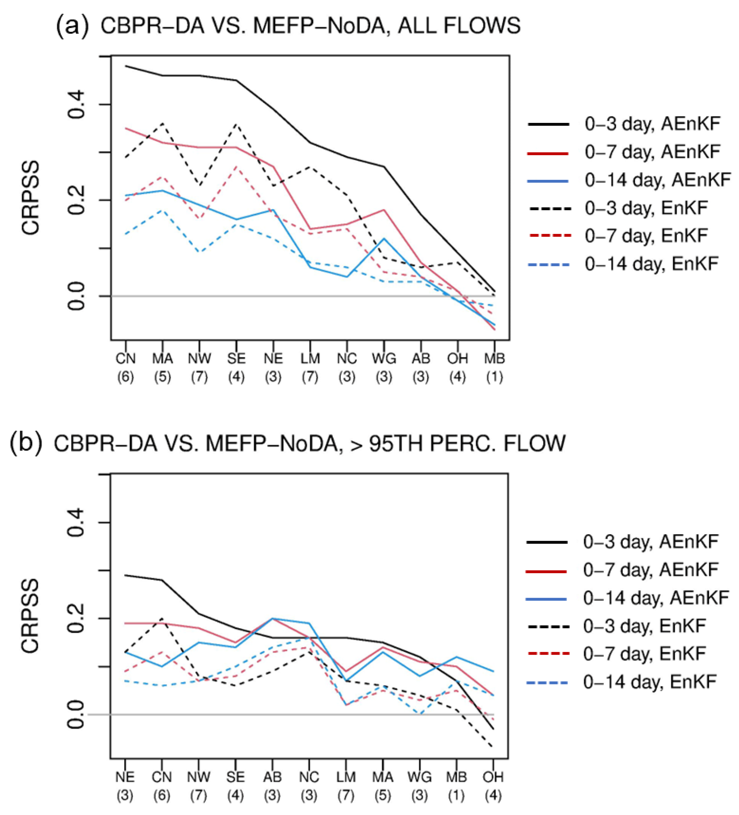
Figure 12a shows the CRPSS of CBPR-DA in reference to MEFP-NoDA for the 11 RFCs represented in the study area for predictions of mean 3-, 7- and 14-day flows over lead times of 0 to 3, 0 to 7 and 0 to 14 days, respectively. Along the x-axis, the number of locations represented is shown in parentheses below the RFC name. The solid and dotted lines are associated with AEnKF and EnKF, respectively. The RFCs are sorted in the descending order of the CRPSS associated with AEnKF for mean 3-day flow over lead times of 0 to 3 days. The lines are drawn to aid visual examination only and have no meaning. Figure 12a shows that, for the prediction of mean 3-day flow over lead times of 0 to 3 days, CBPR-AEnKF reduces mean CRPS of MEFP-NoDA by over 40% for four RFCs (CN, MA, NW and SE) and by over 20% for all but three RFCs (AB, MB and OH). Expectedly, the margin of improvement by CBPR-AEnKF decreases as the lead time increases but still exceeds 10% for the prediction of mean 14-day flow over lead times of 0 to 14 days for all but three RFCs (LM, MB, OH). Comparative evaluation of AEnKF with EnKF has been reported in [35,36,37,40] but is included in Figure 12 for reference. AEnKF and EnKF were run under identical conditions with the identical fixed-lag smoother formulation, parameters and parameter settings. Figure 12a shows that CBPR-AEnKF outperforms CBPR-EnKF by varying margins, and that the margin of improvement is larger for predictions over shorter lead times. The latter is due to the fact that CB tends to be larger and occurs more frequently when the predictors (i.e., observations and model predictions) are subject to larger uncertainties.

Figure 12b is the same as Figure 12a but when conditioned on location-specific observed flow exceeding the 95th percentile. Compared to Figure 12a, CRPSS is significantly smaller which reflects not only the weaker hydrologic memory but also the fact that hydrologic models are calibrated to perform better for high flows. Nevertheless, CBPR-AEnKF improves over MEFP-NoDA by 10% or more even for mean 14-day flow over lead times of 0 to 14 days for all but three RFCs (LM, OH, WG).

4.5. Discussion

Addressing timing errors in streamflow DA remains a challenge [58]. A possible remedial approach may be to account for the uncertainty in the key routing model parameters in the DA process. It is unclear, however, whether real-time streamflow observations have large enough information content to discern timing errors reliably and consistently under widely and dynamically varying flow conditions. Note that incorrect updating of parametric uncertainty will exacerbate the negative impact of timing error. A more holistic approach would be to use DA in a feedback loop for model diagnostics and improvement. For example, strong signs of timing errors may mean that the UHG assumptions are not met consistently and semi-distributed modeling may be necessary [59]. If the DA-updated model states are bounded from above very frequently or their dynamic range is significantly larger than that of the raw model states, model calibration or model physics may need improvement. Similarly, if the DA-updated multiplicative biases for MAP or MAPE are consistently above or below unity, the observed forcings may need correction or improvement. Such analyses will also help identify additional observational needs for streamflow, precipitation and soil moisture. If timing errors cannot be addressed at the source, a practical interim approach is to inflate ${\sigma }_Q$ (see Equation (9)), i.e., pass the hydrologic uncertainty onto streamflow observation uncertainty. Such a practice, however, artificially renders streamflow observations less informative than they actually are and hence dampens the impact of DA.

Future input uncertainty for MAT was ignored in this work in the absence of SWE updating in the hindcast process. For accurate attribution of errors by streamflow DA, it is necessary to include SWE DA in the hindcast process. A significant technical issue in streamflow DA, particularly in cold starts of the DA cycle, is assimilating multiple streamflow observations valid within the same assimilation window. Streamflow is often highly correlated particularly at small time steps. Hence, assimilation of multiple streamflow observations requires highly accurate and robust modeling of flow-dependent observation error covariance which adds complexity. CBPR and streamflow DA described in this work are directed at headwater basins. Given that channel routing has relatively small hydrologic uncertainty, one may postulate that the collective improvement in forecast accuracy for multiple headwater basins by CBPR-DA is very likely to improve forecast accuracy and extend lead time for downstream locations significantly. It is also likely that the above impact is larger for large-scale events that impact a large number of headwater basins. Finally, to fully simulate the operational forecast process and to address a number of the questions raised above effectively, it is necessary to implement streamflow DA in the CHPS. Such an implementation as a plugin via OpenDA [60] has already been demonstrated [61].

As explained in the Introduction Section, the primary purpose of DA is to reduce the IC uncertainty rather than to account for hydrologic uncertainty in its entirety. Hence, DA is not a substitute for ensemble streamflow post-processing but complements post processing and vice versa (see Figure 1). By reducing the IC uncertainty, DA whitens the errors in streamflow simulation by varying degrees. Hence, the use of DA may allow more parsimonious approaches for post-processing which may also reduce data requirements, an important consideration under nonstationarity.

The focus of this work is on the assessment of the impact of CBPR-DA relative to MEFP-NoDA rather than the verification of CBPR-DA in reference to climatological ensemble streamflow forecast. Hence, unlike the MEFP-NoDA results [62], it is not readily possible to compare the CBPR-DA results with those from other ensemble streamflow forecast systems and capabilities (for a review, see [2]). As for MEFP-NoDA, perhaps the most apt comparison is with [63,64], which verify the Australian Bureau of Meteorology’s national operational 7-day ensemble streamflow forecast service for 100 and 96 locations across Australia, respectively, vs. [65], which verifies an early experimental version of the HEFS for five forecast points in north central Texas straddling semi-arid and humid regions. Both systems utilize NWP or NWP-derived forecasts and streamflow post processing and both are verified in reference to climatology. The results are qualitatively similar though, expectedly, there exists large variability in predictive skill from regional and location-to-location variations in the predictability and predictive skill of precipitation and streamflow. Additional work is ongoing for post-processing of DA-aided predictions so that the collective predictive skill in the full HEFS (see Figure 1) may be dissected into component-specific contributions for the 46 locations used in this work. The findings, including the overall accuracy and the competing attributes of reliability and Type II conditional bias [21], will be reported in the very near future. A similar study based on a configuration similar to the full HEFS has recently been reported in [66] for prediction of daily flow for a very large catchment (>15,000 ${\mathrm{k}\mathrm{m}}^2$) in east China.

5. Conclusions and Future Research Recommendations

The potential impact of CBPR-DA on the accuracy of ensemble streamflow forecasts is assessed via 20-yr hindcast experiments. CBPR-DA refers to the combination of the CBPR-aided MEFP and real-time assimilation of streamflow data via AEnKF. The experiments closely follow the operational forecast process and practices at the RFCs. Comparative evaluation of CBPR-DA with MEFP-NoDA is carried out for 46 headwater locations in the service areas of 11 RFCs. MEFP-NoDA refers to the MEFP operation and no streamflow DA and represents the current HEFS operation at the RFCs. The assimilation and forecast cycles used are 6 and 24 h, respectively. The primary performance measures used for the impact assessment are mean CRPS and CRPSS.

The results show that, relative to MEFP-NoDA, CBPR-DA improves the accuracy of ensemble forecasts of mean 3-day flow over lead times of 0 to 3 days by over 40% for 4 RFCs and by over 20% for 9 of the 11 RFCs. In general, the margin of improvement is larger where the predictability of precipitation is larger and hydrologic memory is stronger. Expectedly, the margin of improvement decreases as the lead time increases but still exceeds 10% for the prediction of mean 14-day flow over lead times of 0 to 14 days for all but 3 RFCs. Improvement for high flows is smaller. For verifying observations exceeding the 95th percentile flow for each location, the margin of improvement by CBPR-DA over MEFP-NoDA is over 20% for 3 of the 11 RFCs and over 10% for all but 2 RFCs for prediction of mean 3-day flow over lead times of 0 to 3 days. The findings indicate that, though widely varying from region to region, significant predictability of precipitation and hydrologic memory exist that are not fully utilized in the current operational hydrologic ensemble forecast process. This work offers a potential remedy.

The findings point to the following two issues as most significant for improving CBPR-DA. In the CBPR-aided MEFP, the CBPR coefficient is estimated by incrementally increasing the conditioning cutoff precipitation amount. Whereas this strategy works well for most of the times, it is susceptible to significant estimation errors if the errors in the precipitation forecasts are highly heteroscedastic due to large atmospheric flow-dependent variations in predictive skill. The DA formulation used in this work does not explicitly consider timing errors. If significant timing errors exist, DA is susceptible to incorrect attribution of errors which likely results in forecasts that are out of phase. Section 4.5 identifies additional areas of research. Finally, we note here that work is ongoing to develop a CHPS plugin for streamflow DA and it will be made available to the community on completion.

References

1. Demargne, J.; Wu, L.; Regonda, S.; Brown, J.; Lee, H.; He, M.; Seo, D.-J.; Hartman, R.; Herr, H.; Fresch, M.; et al. The science of NOAA’s operational hydrologic ensemble forecast service. Bull. Am. Meteorol. Soc. 2014, 95, 79–98. [Google Scholar] [CrossRef]
2. Troin, M.; Arsenault, R.; Wood, A.W.; Brissette, F.; Martel, J.-L. Generating ensemble streamflow forecasts: A review of methods and approaches over the past 40 years. Water Resour. Res. 2021, 57, e2020WR028392. [Google Scholar] [CrossRef]
3. Krzysztofowicz, R. Bayesian theory of probabilistic forecasting via deterministic hydrologic model. Water Resour. Res. 1999, 35, 2739–2750. [Google Scholar] [CrossRef]
4. Seo, D.-J.; Herr, H.; Schaake, J. A statistical post-processor for accounting of hydrologic uncertainty in short-range ensemble streamflow prediction. Hydrol. Earth Syst. Sci. Discuss. 2006, 3, 1987–2035. [Google Scholar]
5. Schaake, J.; Demargne, J.; Mullusky, M.; Welles, E.; Wu, L.; Herr, H.; Fan, X.; Seo, D.-J. Precipitation and temperature ensemble forecasts from single-value forecasts. Hydrol. Earth Syst. Sci. 2007, 4, 655–717. [Google Scholar]
6. Wu, L.; Seo, D.-J.; Demargne, J.; Brown, J.D.; Cong, S.; Schaake, J. Generation of ensemble precipitation forecast from single-valued quantitative precipitation forecast for hydrologic ensemble prediction. J. Hydrol. 2011, 399, 281–298. [Google Scholar] [CrossRef]
7. National Weather Service. MEFPPE Configuration Guide; NOAA/NWS/Office of Water Prediction: Silver Spring, MD, USA, 2022. Available online: https://vlab.noaa.gov/documents/207461/1893010/MEFPPEConfigurationGuide.pdf (accessed on 13 August 2025).
8. National Weather Service. Meteorological Ensemble Forecast Processor (MEFP) User’s Manual; NOAA/NWS/Office of Water Prediction: Silver Spring, MD, USA, 2022. Available online: https://vlab.noaa.gov/documents/207461/1893026/MEFP_Users_Manual.pdf (accessed on 13 August 2025).
9. Cui, B.; Toth, Z.; Zhu, Y.; Hou, D. Bias correction for global ensemble forecast. Weather Forecast. 2012, 27, 396–410. [Google Scholar] [CrossRef]
10. Whitin, B.; He, K. MEFP Large Precipitation Event Analysis; California-Nevada River Forecast Center, NWS: Sacramento, CA, USA, 2015.
11. Seo, D.-J.; Kim, S.; Alizadeh, B.; Limon, R.A.; Ghazvinian, M.; Lee, H. Improving Precipitation Ensembles for Heavy-to-Extreme Events and Streamflow Post-Processing for Short-to-Long Ranges; Department of Civil Engineering, University of Texas at Arlington: Arlington, TX, USA, 2019; 52p. [Google Scholar]
12. Jozaghi, A.; Shen, H.; Ghazvinian, M.; Seo, D.-J.; Zhang, Y.; Welles, E.; Reed, S. Multi-model streamflow prediction using conditional bias-penalized multiple linear regression. Stoch. Environ. Res. Risk Assess. 2021, 35, 2355–2373. [Google Scholar] [CrossRef]
13. Kim, S.; Jozaghi, A.; Seo, D.-J. Improving ensemble forecast quality for heavy-to-extreme precipitation for the Meteorological Ensemble Forecast Processor via conditional bias-penalized regression. J. Hydrol. 2025, 647, 132363. [Google Scholar] [CrossRef]
14. Kim, S.; Seo, D.-J. Comparative evaluation of conditional bias-penalized regression-aided Meteorological Ensemble Forecast Processor for large-to-extreme precipitation events. Weather Forecast. 2025, 40, 959–975. [Google Scholar] [CrossRef]
15. Alizadeh, B. Improving Post Processing of Ensemble Streamflow Forecast for Short-to-Long Ranges: A Multiscale Approach. Ph.D. Thesis, University of Texas at Arlington, Arlington, TX, USA, 2019; 125p. [Google Scholar]
16. Alizadeh, B.; Limon, R.A.; Seo, D.; Lee, H.; Brown, J. Multiscale postprocessor for ensemble streamflow prediction for short to long ranges. J. Hydrometeorol. 2020, 21, 265–285. [Google Scholar] [CrossRef]
17. Mendoza, P.; Wood, A.; Clark, E.; Nijssen, B.; Clark, M.; Ramos, M.-H.; Voisin, N. Improving medium-range ensemble streamflow forecasts through statistical post-processing. In Proceedings of the 2016 American Geophysical Union Fall Meeting, San Francisco, CA, USA, 12–16 December 2016. [Google Scholar]
18. National Weather Service. The Experimental Ensemble Forecast System (XEFS) Design and Gap Analysis; NOAA/NWS/Office of Hydrologic Development: Silver Spring, MD, USA, 2007; 50p.
19. Hornberger, G.; Raffensperger, J.P.; Wiberg, P.L.; Eshleman, K.N. Elements of Physical Hydrology; Johns Hopkins University Press: Baltimore, MD, USA, 1998. [Google Scholar]
20. Hersbach, H. Decomposition of the continuous ranked probability score for ensemble prediction systems. Weather Forecast. 2000, 15, 559–570. [Google Scholar] [CrossRef]
21. World Meteorological Organization. Guidelines on the Verification of Hydrological Forecasts; WMO: Geneva, Switzerland, 2025; 197p. [Google Scholar]
22. Lee, H.S.; Liu, Y.; Brown, J.; Ward, J.; Maestre, A.; Fresch, M.A.; Herr, H.; Wells, E. Validation of ensemble streamflow forecasts from the Hydrologic Ensemble Forecast Service (HEFS). In Proceedings of the American Geophysical Union 2018 Fall Meeting, Washington, DC, USA, 10–14 December 2018. [Google Scholar]
23. Lee, H.S.; Liu, Y.; Ward, J.; Kim, S.; Brown, J.; Maestre, A.; Fresch, M.A.; Herr, H.; Wells, E.; Camacho, F. On the improvements in precipitation, temperature and streamflow forecasts from the Hydrologic Ensemble Forecast Service after upgrading from the GEFSv10 to the GEFSv12. In Proceedings of the American Geophysical Union 2020 Fall Meeting, Virtual, 1–17 December 2020. [Google Scholar]
24. Guan, H.; Zhu, Y.; Sinsky, E.; Fu, B.; Li, W.; Zhou, X.; Xue, X.; Hou, D.; Peng, J.; Nageswararao, M.M.; et al. GEFSv12 reforecast dataset for supporting subseasonal and hydrometeorological applications. Mon. Weather Rev. 2022, 150, 647–665. [Google Scholar] [CrossRef]
25. Hamill, T.M.; Whitaker, J.S.; Shlyaeva, A.; Bates, G.; Fredrick, S.; Pegion, P.; Sinsky, E.; Zhu, Y.; Tallapragada, V.; Guan, H.; et al. The Reanalysis for the Global Ensemble Forecast System, Version 12. Mon. Weather Rev. 2022, 150, 59–79. [Google Scholar] [CrossRef]
26. Roe, J.; Dietz, C.; Restrepo, P.; Halquist, J.; Hartman, R.; Horwood, R.; Olsen, B.; Opitz, H.; Shedd, R.; Welles, E. NOAA’s Community Hydrologic Prediction System. In Proceedings of the Second Joint Federal Interagency Conference, Las Vegas, NV, USA, 27 June–1 July 2010; 12p. [Google Scholar]
27. Burnash, R.J.C.; Ferral, R.L.; McGuire, R.A. A Generalized Streamflow Simulation System—Conceptual Modeling for Digital Computers. National Weather Service, NOAA, and the State of California Department of Water Resources Technical Report; Joint Federal-State River Forecast Center: Sacramento, CA, USA, 1973; 68p.
28. Anderson, E.A. A Point Energy and Mass Balance Model of a Snow Cover. NOAA Technical Report; NWS: Silver Spring, MD, USA, 1976; Volume 19, 150p. [Google Scholar]
29. Chow, V.T.; Maidment, D.R.; Mays, L.W. Applied Hydrology; McGraw-Hill: New York, NY, USA, 1988. [Google Scholar]
30. Seo, D.-J.; Cajina, L.; Corby, R.; Howieson, T. Automatic state updating for operational streamflow forecasting via variational data assimilation. J. Hydrol. 2009, 367, 255–275. [Google Scholar] [CrossRef]
31. Bissell, V.C. When NWSRFS, SEUS and Snow Intersect. In Proceedings of the Western Snow Conference, Bend, OR, USA, 16–18 April 1996. [Google Scholar]
32. Franz, K.; Hogue, T.; Barik, M.; He, M. Assessment of SWE data assimilation for ensemble streamflow predictions. J. Hydrol. 2014, 519 Pt D, 2737–2746. [Google Scholar] [CrossRef]
33. Moser, C.L.; Kroczynski, S.; Hlywiak, K. Comparison of the SAC-SMA and API-CONT Hydrologic Models at Several Susquehanna River Headwater Basins. Eastern Region Technical Attachment No. 2013-01. 2013; 20p. Available online: https://www.weather.gov/media/erh/ta/ta2013-01.pdf (accessed on 13 August 2025).
34. Kuzmin, V.; Seo, D.-J.; Koren, V. Fast and efficient optimization of hydrologic model parameters using a priori estimates and stepwise line search. J. Hydrol. 2008, 353, 109–128. [Google Scholar] [CrossRef]
35. Seo, D.-J.; Shen, H.; Lee, H. Adaptive conditional bias-penalized Kalman filter with minimization of degrees of freedom for noise for superior state estimation and prediction of extremes. Comput. Geosci. 2022, 166, 105193. [Google Scholar] [CrossRef]
36. Shen, H.; Lee, H.; Seo, D.-J. Adaptive conditional bias-penalized Kalman filter for improved estimation of extremes and its approximation for reduced computation. Hydrology 2022, 9, 35. [Google Scholar] [CrossRef]
37. Shen, H.; Seo, D.-J.; Lee, H.; Liu, Y.; Noh, S. Improving flood forecasting using conditional bias-aware assimilation of streamflow observations and dynamic assessment of flow-dependent information content. J. Hydrol. 2022, 605, 127247. [Google Scholar] [CrossRef]
38. Jozaghi, A.; Shen, H.; Seo, D.-J. Adaptive conditional bias-penalized kriging for improved spatial estimation of extremes. Stoch. Environ. Res. Risk Assess. 2024, 38, 193–209. [Google Scholar] [CrossRef]
39. Seo, D.-J. Conditional bias-penalized kriging. Stoch. Environ. Res. Risk Assess. 2013, 27, 43–58. [Google Scholar] [CrossRef]
40. Lee, H.; Noh, S.; Kim, S.; Shen, H.; Seo, D.-J.; Zhang, Y. Improving flood forecasting using conditional bias-penalized ensemble Kalman filter. J. Hydrol. 2019, 575, 596–611. [Google Scholar] [CrossRef]
41. Schweppe, F.C. Uncertain Dynamic Systems; Prentice-Hall: Englewood Cliffs, NJ, USA, 1973; 563p. [Google Scholar]
42. Wilks, D.S. Statistical Methods in the Atmospheric Sciences; Elsevier Academic Press: San Diego, CA, USA, 2006; 648p. [Google Scholar]
43. Seo, D.-J.; Mohammad Saifuddin, M.; Lee, H. Conditional bias-penalized Kalman filter for improved estimation and prediction of extremes. Stoch. Environ. Res. Risk Assess. 2017, 32, 183–201. [Google Scholar] [CrossRef]
44. Kalman, R.E. A new approach to linear filtering and prediction problems. J. Basic Eng. 1960, 82, 35. [Google Scholar] [CrossRef]
45. Evensen, G. Sequential data assimilation with nonlinear quasi-geostrophic model using Monte Carlo methods to forecast error statistics. J. Geophys. Res. 1994, 99, 143–162. [Google Scholar] [CrossRef]
46. Lorentzen, R.J.; Naevdal, G. An iterative ensemble Kalman filter. IEEE Trans. Autom. Control 2011, 56, 1990–1995. [Google Scholar] [CrossRef]
47. Rodgers, C.D. Inverse Methods for Atmospheric Sounding: Theory and Practice; World Scientific: Singapore, 2000. [Google Scholar] [CrossRef]
48. Sorooshian, S.; Dracup, J.A. Stochastic parameter estimation procedures for hydrologic rainfall–runoff models: Correlated and heteroscedastic error cases. Water Resour. Res. 1980, 16, 430–442. [Google Scholar] [CrossRef]
49. Carpenter, T.M.; Georgakakos, K.P. Impacts of parametric and radar rainfall uncertainty on the ensemble streamflow simulations of a distributed hydrologic model. J. Hydrol. 2004, 298, 202–221. [Google Scholar] [CrossRef]
50. Weerts, A.H.; El Serafy, G.Y. Particle filtering and ensemble Kalman filtering for state updating with hydrological conceptual rainfall–runoff models. Water Resour. Res. 2006, 42, W09403. [Google Scholar] [CrossRef]
51. Clark, M.P.; Rupp, D.E.; Woods, R.A.; Zheng, X.; Ibbitt, R.P.; Slater, A.G.; Schmidt, J.; Uddstorm, M.J. Hydrologic data assimilation with the ensemble Kalman filter: Use of streamflow observations to update states in a distributed hydrological model. Adv. Water Resour. 2008, 31, 1309–1324. [Google Scholar] [CrossRef]
52. Rakovec, O.; Weerts, A.H.; Hazenberg, P.; Torfs, P.J.J.F.; Uijlenhoet, R. State updating of a distributed hydrological model with Ensemble Kalman Filtering: Effects of updating frequency and observation network density on forecast accuracy. Hydrol. Earth Syst. Sci. 2012, 16, 3435–3449. [Google Scholar] [CrossRef]
53. National Weather Service. NWSRFS User Manual Documentation; Office of Water Prediction: Silver Spring, MD, USA, 2024.
54. Bowler, N.E. Accounting for the effect of observation errors on verification of MOGREPS. Meteorol. Appl. 2008, 15, 199–205. [Google Scholar] [CrossRef]
55. Bellier, J.; Zin, I.; Bontron, G. Sample stratification in verification of ensemble forecasts of continuous scalar variables: Potential benefits and pitfalls. Mon. Weather Rev. 2017, 145, 3529–3544. [Google Scholar] [CrossRef]
56. Lerch, S.; Thorarinsdottir, T.L.; Ravazzolo, F.; Gneiting, T. Forecaster’s Dilemma: Extreme Events and Forecast Evaluation. Stat. Sci. 2017, 32, 106–127. [Google Scholar] [CrossRef]
57. Moore, B.J. Flow dependence of medium-range precipitation forecast skill over California. Weather Forecast. 2023, 38, 699–720. [Google Scholar] [CrossRef]
58. Noh, S.; Weerts, A.; Rakovec, O.; Lee, H.; Seo, D.-J. Assimilation of streamflow observations. In Handbook of Hydrometeorological Ensemble Forecasting; Duan, Q., Pappenberger, F., Thielen, J., Wood, A., Cloke, H.L., Schaake, J.C., Eds.; Springer: Berlin/Heidelberg, Germany, 2018. [Google Scholar] [CrossRef]
59. Smith, M.; Koren, V.; Zhang, Z.; Reed, S.; Seo, D.-J.; Moreda, F.; Kuzmin, V.; Cui, Z.; Anderson, R. NOAA NWS Distributed Hydrologic Modeling Research and Development. NOAA Technical Report; NWS: Silver Spring, MD, USA, 2004; Volume 51, 63p.
60. van Velzen, N.; Altaf, M.U.; Verlaan, M. OpenDA-NEMO framework for ocean data assimilation. Ocean Dyn. 2016, 66, 691–702. [Google Scholar] [CrossRef][Green Version]
61. Kim, S.; Shen, H.; Noh, S.; Seo, D.-J.; Welles, E.; Pelgrim, E.; Weerts, A.; Lyons, E.; Philips, B.; Smith, M.; et al. High-resolution modelling and prediction of urban floods using WRF-Hydro and data assimilation. J. Hydrol. 2020, 598, 126236. [Google Scholar] [CrossRef]
62. Brown, J.D.; He, M.; Regonda, S.; Wu, L.; Lee, H.; Seo, D.-J. Verification of temperature, precipitation and streamflow forecasts from the NOAA/NWS Hydrologic Ensemble Forecast Service (HEFS): 2. Streamflow verification. J. Hydrol. 2014, 519 Pt D, 2847–2868. [Google Scholar] [CrossRef]
63. Hapuarachchi, H.A.P.; Bari, M.A.; Kabir, A.; Hasan, M.M.; Woldemeskel, F.M.; Gamage, N.; Sunter, P.D.; Zhang, X.S.; Robertson, D.E.; Bennett, J.C.; et al. Development of a national 7-day ensemble streamflow forecasting service for Australia. Hydrol. Earth Syst. Sci. 2022, 26, 4801–4821. [Google Scholar] [CrossRef]
64. Bari, M.A.; Hasan, M.M.; Amirthanathan, G.E.; Hapuarachchi, H.A.P.; Kabir, A.; Cornish, A.D.; Sunter, P.; Feikema, P.M. Performance Evaluation of a National Seven-Day Ensemble Streamflow Forecast Service for Australia. Water 2024, 16, 1438. [Google Scholar] [CrossRef]
65. Kim, S.; Sadeghi, H.; Limon, R.A.; Seo, D.-J.; Philpott, A.; Bell, F.; Brown, J.; He, K. Ensemble streamflow forecasting using short- and medium-range precipitation forecasts for the Upper Trinity River Basin in North Texas via the Hydrologic Ensemble Forecast Service (HEFS). J. Hydrometeorol. 2018, 19, 1467–1483. [Google Scholar] [CrossRef]
66. Zhang, J.; Li, W.; Duan, Q. Quantifying the contributions of hydrological pre-processor, post-processor, and data assimilator to ensemble streamflow prediction skill. J. Hydrol. 2025, 651, 132611. [Google Scholar] [CrossRef]
Figure 1. Schematic of the full HEFS (Adapted with permission from [1]. 2014, American Meteorological Society). The four main science components are shown in rectangular boxes.
Hydrology 12 00229 g001
Figure 2. Map of the study area.
Hydrology 12 00229 g002
Figure 3. Data flows for the hindcast experiments (righthand side) and the Adjoint-Based OPTimizer (AB_OPT) (lefthand side, adapted from [30]. 2009, Elsevier).
Hydrology 12 00229 g003
Figure 4. CRPSS of MEFP-DA in reference to MEFP-NoDA for observed flows exceeding (a) 0th, (b) 90th, (c) 95th and (d) 99th percentiles for all locations.
Hydrology 12 00229 g004
Figure 5. The 6-h empirical UHGs for (a) GLML1 and (b) PICT2.
Hydrology 12 00229 g005
Figure 6. Mean CRPS of MEFP-NoDA, MEFP-DA and CBPR-DA conditional on verifying observed flow exceeding the 99th percentile for (a) GLML1 and (b) PICT2.
Hydrology 12 00229 g006
Figure 7. Same as Figure 4 but for CBPR-NoDA in reference to MEFP-NoDA for observed flows exceeding (a) 0th, (b) 90th, (c) 95th and (d) 99th percentiles for all locations.
Hydrology 12 00229 g007
Figure 8. Same as Figure 4 but for CBPR-DA in reference to MEFP-NoDA for observed flows exceeding (a) 0th, (b) 90th, (c) 95th and (d) 99th percentiles for all locations.
Hydrology 12 00229 g008
Figure 9. C R P S M E F P N o D A C R P S C B P R D A vs. verifying observation between the lead times of 0 and 7 days for all 46 locations.
Hydrology 12 00229 g009
Figure 10. CRPSS of CBPR-DA of (a) 3- and (b) 7-day streamflow forecast in reference to MEFP-NoDA for observed flows exceeding 0th, 90th, 95th and 99th percentiles for all locations.
Hydrology 12 00229 g010aHydrology 12 00229 g010b
Figure 11. Scatter (crosses) and quantile-quantile (red solid lines) plots of 3-day ensemble mean forecasts over lead times of 0 to 3 days from MEFP-NoDA (left panels) and CBPR-DA (right panels) for (a) AB-, (b) CN-, (c) LM-, (d) NW-, (e) SE- and (f) WGRFC locations. One-to-one lines are in solid gray.
Hydrology 12 00229 g011aHydrology 12 00229 g011b
Figure 12. CRPSS of CBPR-DA of mean 3-, 7- and 14-day streamflow forecasts over lead times of 0 to 3, 0 to 7 and 0 to 14 days in reference to MEFP-NoDA without post-factum correction of input bias, refinement of UHG and local optimization of SAC parameters for all locations in each RFC in the study area (a) for all verifying observed flow and (b) for verifying observed flow exceeding the 95th percentile.
Hydrology 12 00229 g012
Disclaimer/Publisher’s Note: The statements, opinions and data contained in all publications are solely those of the individual author(s) and contributor(s) and not of MDPI and/or the editor(s). MDPI and/or the editor(s) disclaim responsibility for any injury to people or property resulting from any ideas, methods, instructions or products referred to in the content.