Challenges and Limitations of Using Monitoring Data in Catchment-Based Models—A Case Study of Rivers Taw and Torridge, UK

Abstract

Water quality monitoring is a key requirement for fulfilling various national environmental policies, but with many competing needs and limited resources, data collected can suffer from both spatial and temporal deficiencies. Modelling offers the potential to substitute estimated values into observational gaps, but model validation often requires the very data that are lacking. In this paper we present the results of a pilot study to investigate spatial and temporal issues around the monitoring of faecal indicator bacteria (Escherichia coli) in rivers of the Taw and Torridge catchments in the UK. Statistical analysis of in situ measurements versus simulated data from the catchment models reveals similar seasonal associations between riverine bacterial counts and rainfall patterns. Furthermore, spatial apportionment of livestock to better reflect land use was found to be important in the models, especially in upstream reaches of the catchments. In conclusion, successful monitoring of faecal bacteria levels in UK rivers requires risk-based monitoring (sufficient to identify possible seasonal trends) and informed spatial consideration of sampling sites. Catchment models can be useful aids for directing and augmenting such monitoring programmes, but these models should undergo rigorous validation, particularly in upper catchment areas, to ensure correct model response to changes in land use and/or climate.

1. Introduction

National statutory bodies responsible for monitoring water quality within water bodies must fulfil many, often competing and changing, policy objectives. To fulfil their remit, national monitoring programmes must be designed to have adequate spatial and temporal coverage for reliable assessment of water quality standards, while keeping costs of sample collection and analysis within reasonable limits. Primarily (though not exclusively), the aims of such programmes are to protect human health and prevent environmental degradation. In certain cases, water quality may be monitored more frequently, for example, to assess the cause of suspected deterioration or contamination events, or to examine the effectiveness of long-term environmental improvement measures. However, in the absence of specific needs, financial and human resource constraints limit the capacity for high-resolution monitoring throughout the national waterbody network; therefore, data are rarely available at a sufficiently high spatial resolution or temporal frequency to inform the implementation of site-specific measures to support a healthy aquatic environment. Additionally, there is no spatial or temporal uniformity to current routine monitoring at the river catchment level, and it is common to find large gaps in spatial and temporal records. Often, this leads to mitigative measures having to be put in place once negative impacts (e.g., disease outbreaks in human or animal populations; environmental degradation) are observed [1,2].

To assist with estimation of water quality in data-limited areas, models at the scale of individual river catchments have the potential to be used in combination with in situ monitoring data to assess the environmental characteristics and human activities that are likely to have the greatest influence on water quality. Such tools can help environmental managers understand both spatial and temporal variations in the sources and loadings of various substances entering watercourses, including nutrients, sediments, chemical compounds, and pathogenic organisms.

In England and Wales, there is a strong focus on hydrological and physico-chemical monitoring of water bodies. River flow gauges capture hydrological data, which are examined against historical records to identify and interpret emerging hydrological trends over time. The findings are used to improve water management strategies, increase awareness of water resources issues, and assess and report on flood and drought risk. Although the Environment Agency routinely monitors physico-chemical parameters (e.g., temperature, turbidity, pH, dissolved oxygen, and nitrates), monitoring of individual parameters can be sporadic and limited in certain locations. Additionally, few measurements relate to bacterial content, and monitoring of the faecal indicator Escherichia coli (E. coli) tends to be restricted to bathing waters, most of which are in coastal marine, rather than inland freshwater, locations: this is carried out only between March and October, during the UK ‘bathing season’, to protect human health. Other bacterial monitoring tends to be on a case basis, e.g., to support classification of shellfish harvesting areas for food safety purposes.

Faecal indicator bacteria, such as E. coli, faecal coliforms, and enterococci, are used globally as proxies for the presence of faecally derived pathogens in freshwater bodies [3]. Consequently, the use of high-quality monitoring data for these indicators as inputs to high-resolution catchment models can assist decision-making around effective mitigation measures for environmental improvement and protection of human health. Catchment models have become increasingly advanced and more widely available, resulting in a wealth of studies on estimating changes in surface run-off and water yield for flood mitigation and soil erosion purposes [4,5] and estimating chemical loadings, including nutrients, to riverine environments [6,7]. Incorporation of the fate of microbial or faecal indicator organisms is often less well advanced and, therefore, there are typically fewer studies on the assessment of the fate of bacterial loadings to waterbodies [8,9]. Faecal contamination of freshwater, estuarine and coastal waters can have various causes, but principal sources are faecal matter from humans (e.g., via point source wastewater discharges), agricultural livestock (e.g., via diffuse run-off from agricultural land), and wildlife (via direct deposition into waterbodies or diffuse terrestrial run-off). The magnitude and extent of both point source discharges and diffuse inputs can be influenced by environmental factors, such as topography and rainfall. For example, it is well known that episodic bacterial loads occur, often because of high flow conditions due to storm rainfall events [10]. As a result, the tracing of sources and subsequent transmission pathways of microbiological pathogens is complex, not least due to their spatial and temporal variability. Therefore, successful reduction and mitigation of the negative impacts of such pathogens require routine detailed observation and analysis to enable predictive and mitigative measures to be focused effectively.

The work presented here formed one element of a wider project under the Pathogen Surveillance in Agriculture, Food and Environment (PATH-SAFE) programme [11], which examined potential sources and pathways of pathogens implicated in foodborne disease. Although the programme focused on foodborne disease risk, the work has wider application to situations where microbial contamination of waterbodies poses a risk to human, animal or ecosystem health [12,13]. Through a case study at the scale of a river catchment in southwest England [14], the work investigated how microbiological contaminants, from both diffuse and point sources, could be transported via overland run-off and watercourses to adjacent coastal waters, where high levels of microbiological contamination could pose a potential human health risk. The aim was to better understand pathogen transport and loadings in various parts of the river network, under different seasonal conditions, and to identify possible gaps and limitations in the existing monitoring framework, to provide recommendations for application to the national surveillance network.

SWAT (Soil and Water Assessment Tool) is a river basin hydrologic model used to simulate water flow, and nutrient and sediment mass transport, within a defined watershed [15]. The model has been used extensively in studies worldwide to assess the influence of land use change [16,17], farm management practices [18], and climate change [17,19] on water availability and nutrient contamination. More recently, the model has been used to model salinity changes [20,21] and microbial loads within river catchments [22,23]. Conceptually, the SWAT model is a continuous model, typically operating on a daily time scale, simulating water, transport processes of nutrients and other components (such as pesticides and bacteria) in surface run-off, soil percolation, soil lateral flow, groundwater flow with discharge to streams, and stream flow. Its approach is to divide a watershed into subbasins connected via a stream network. These subbasins are then divided into hydrological response units (HRUs), each representing a unique combination of land use, soil type, and topographic slope. Vegetative growth, management practices, and hydrology are simulated at the level of the HRU, driven by input data on climatic conditions (precipitation, temperature, humidity, solar radiation and wind), land use operations (for example, the application of fertilizer), and regional soil properties. At the level of the HRU, water, nutrients, sediment and other constituents (such as pesticides) are summarized and routed through the watershed via the stream network, eventually reaching the watershed outlet.

In addition, SWAT 2012 integrates a bacterial module that enables the fate and transport of two types of bacterial populations to be modelled concurrently, namely persistent and non-persistent bacteria. This allows bacterial (or viral) populations with distinct growth and die-off patterns to be incorporated, enabling separate consideration of bacteria that persist in the soil and those that do not. The bacterial module of SWAT includes the ability to incorporate loadings from a variety of sources, including livestock, wildlife, point sources (such as water company sewage discharges), and septic systems of private dwellings. Equations are employed to control the movement of bacteria from land to the stream network, and to model bacterial die-off and regrowth within the watercourse (reach) of each subbasin. Bacteria can enter the watercourse through surface run-off, especially important during rainfall events, or via sediment transport and/or resuspension from streambed sediments. The SWAT model assumes that bacteria present in the top 10 mm of the soil are available for transport under run-off conditions, and transport of bacteria via groundwater to streams is not considered, with bacteria in groundwater assumed to be lost to the system.

Using this case study as an example, our paper examines the challenge of combining diverse environmental data within a river catchment model to estimate diffuse and point source bacterial inputs into, and transport through, the system, with the aim of obtaining a close approximation to observed microbiological loadings. The following challenges are investigated and explored in this paper:

Challenge 1: Monitoring data on bacterial concentrations in riverine water are typically sparse both temporally and spatially. For the Taw and Torridge catchments, is seasonal variation evident within the monitored data, and how does it respond to rainfall events within the catchment?

Challenge 2: Often, livestock numbers for cattle and sheep are apportioned equally across a catchment by land use. Does the spatial apportionment of livestock to specific areas within the catchment result in a significant improvement in modelling of bacteria?

Challenge 3: An effective catchment model should respond in a similar manner to observed data measured in the catchment. Does the bacterial modelling within SWAT respond in a similar way to rainfall events as seen in the monitoring data?

2. Materials and Methods

2.1. Study Area

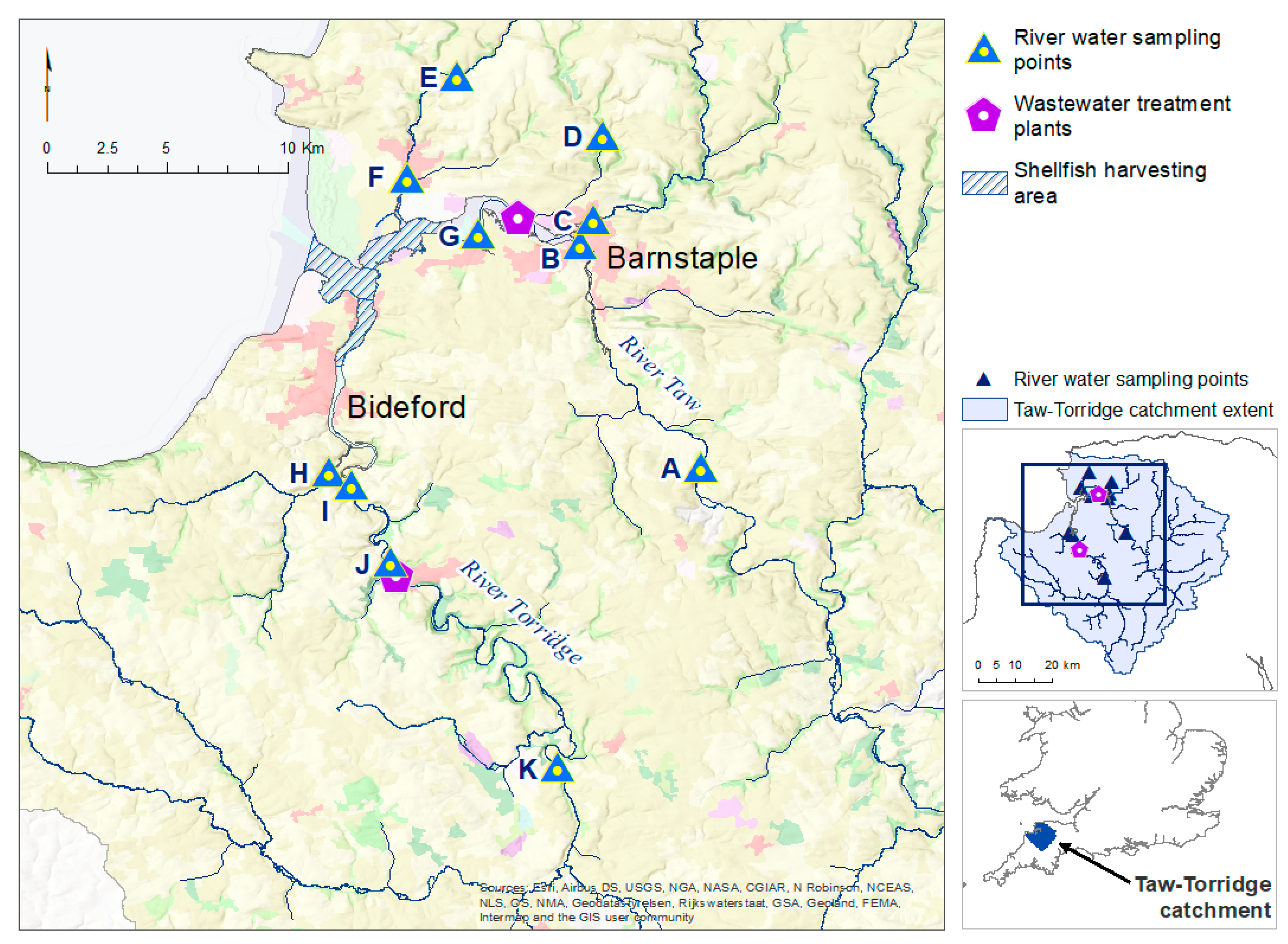
The study focused on the combined catchments of the Rivers Taw and Torridge in north Devon (Figure 1), a largely rural area, with the small towns of Barnstaple (on the Taw) and Bideford (on the Torridge) being the main conurbations upstream of the Taw estuary. Agricultural grasslands dominate the catchments, interspersed with small pockets of arable farming and mixed woodland at lower elevations, with peatland confined to higher ground where the River Taw rises in the south, within Dartmoor National Park. There are saltmarshes along the banks of the estuary, and large expanses of mudflats and sandbanks form an important habitat for overwintering and migratory wading birds. The estuary includes an area important for shellfish harvesting for human consumption, and the outer estuarine and coastal waters are popular for recreational sailing and bathing activities.

The agricultural grasslands are largely used for grazing cattle and sheep, forming a potential source and route for diffuse microbiological contamination from livestock faeces and manures to enter the watercourses via agricultural run-off. Additionally, outflows from sewage treatment works (STWs) and sewer overflows (SOs), which are point sources of human-derived contaminants entering the watercourses, are distributed throughout both catchments.

The strong maritime environment of southwest England usually prevents very low temperatures and limits the annual temperature range. Altitude is the main influencing factor away from the coast, as temperature decreases with height, e.g., an annual mean temperature of 11–12 °C on the Devon coast, compared with 8.5 °C on Dartmoor. Rainfall totals across Devon are also driven by the topography, with altitude rising from sea level to over 600 m on the granite outcrops of Dartmoor. Monthly rainfall is very variable across the county, and total annual values can range from 900 to 1000 m in coastal areas to double this value in upland locations [24].

A flow diagram of the study set-up and analysis can be found in the Supplementary Materials Figure SA1.

2.2. Measurement of Bacteria Counts in Riverine Samples

River water samples were collected weekly from 11 sampling locations (Sites A–G in the Taw and H–K in the Torridge; Figure 1) over two separate 3-month periods, January to March, and June to August, 2023. Streamflow during the ‘winter’ period consisted of an initial high flow period during the first 2 weeks followed by a prolonged ‘low’ flow period with rates below those of the historical mean flow rate, and a final 4 week period of higher flows (see Supplementary Materials Figure SB1 for more details). The summer period saw a typical low flow regimen with a slight increase in flow in the last 2 weeks.

Sites were selected to provide a good spatial distribution, and were located along main river channels and tributaries leading to the Taw estuary, covering a range of land use types (from rural to urban) and, where access was possible, were situated upstream and downstream of conurbations, main river confluences and/or wastewater outlets. River water samples were collected and transported using sterile apparatus, taking care to avoid contamination, according to protocols used for sampling waters in shellfish production areas [25]. Water temperature was recorded at each collection point, and samples were stored at 4 °C prior to analysis the following day, according to standard Environment Agency protocols for water quality testing.

For quantification of E. coli, the water samples (10 mL, 1 mL, and 0.1 mL) were filtered through a 0.45 µm 47 mm diameter filter membrane. Volumes below 10 mL were resuspended in 10 mL Ringer ¼ strength solution before filtration. The filter membrane was placed onto a TBX agar plate, recovered at 30 °C for 4 h, and then incubated at 44 °C overnight. Blue-green colonies were counted as E. coli and the final concentrations were calculated as colony-forming units (cfu) per 100 mL.

2.3. Catchment Modelling Using the Soil and Water Assessment Tool (SWAT)

Although both rivers discharge to the same estuary, separate SWAT models were generated for the respective Taw and Torridge river catchments, enabling independent refinement and calibration of each model, and decreasing processing time while generating and running the models.

Construction of the SWAT model was performed using the ArcSWAT plugin (version 2012.10_5_24) for ArcMap 10.5 [26] and the model was run with the SWAT 2012 Editor interface 2012.10_7.23, using the SWAT executable Rev_692_64rel.exe. The GIS layers used in model construction are shown in Supplementary Materials Table SC1 [27,28,29,30]. Observed weather data from the UK Met Office (Supplementary Materials Table SC2) for the period 01/01/2010 to 31/12/2023 [31,32] were processed in R v4.2.2 [33] to the required format to run in the SWAT 2012 model.

Sensitivity analysis and calibration of the model were performed using the R package ‘R-SWAT’ (version v1.0.0) [34]. Sensitivity analysis using the uniform Latin Hypercube sampling approach identified 9 parameters for calibration of river flow (detailed in Supplementary Materials Table SC3), which were run under an automated calibration process using a Dynamically Dimensioned Search algorithm. This algorithm was used to obtain the best estimates for these parameters, by maximizing the Kling-Gupta Efficiency (KGE) measure [35] between modelled and observed discharge flows. Calibration was performed using river flow data obtained from the National River Flow Archive (NRFA) [36].

2.4. Spatially Distributed Land Use and Land Management Practices

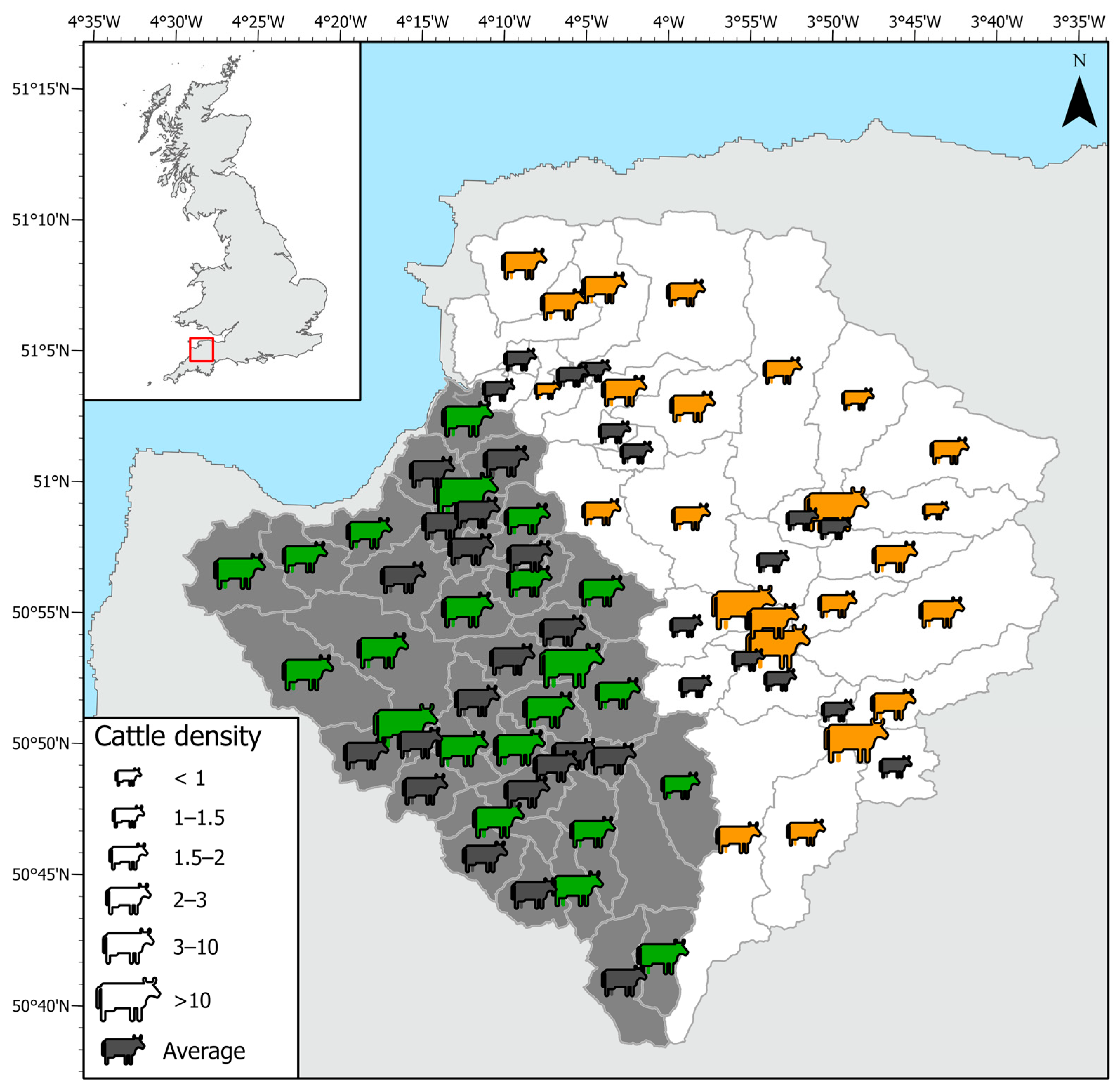
Livestock and dairy production in the Taw catchment typically involve pasture grazing from late spring through late autumn, with winter and early spring housing. Sheep are grazed outdoors, apart from a short winter and early spring housing period for lambing. Livestock numbers for farms, aggregated at subbasin level within the area covered by the Taw and Torridge catchment models, were obtained by request from the Defra June Survey of Agriculture for 2021 [37], and were applied to the analysis in two different ways. In the first (non-spatial apportionment) approach, individual animals per species of interest (cattle and sheep)—hereafter referred to as livestock units (LU)—were summed for each catchment and used to calculate the overall catchment livestock density (LU ha⁻¹). For each species, this value was distributed evenly across improved pastureland (all cattle and 50% of sheep) and pastureland (the remaining 50% of sheep) as estimates of livestock present on those land cover classes. In the second (spatial apportionment) approach, the aggregated livestock numbers obtained were used to calculate LU ha⁻¹ for most subbasins (see Figure 2); however, due to privacy restrictions, livestock numbers were unavailable for subbasins with fewer than 5 farms, so the density of those subbasins was set to the overall density estimated using the non-spatial apportionment approach. It should also be noted that spatial distribution at the subbasin level assumes that livestock are reared close to the holding to which the data are attributed.

Using the estimates of livestock density, the total mass of dry manure and slurry was calculated for each subbasin; the total values for both catchments are shown in

Table 1. Livestock density and manure production in the Taw and Torridge catchments. Livestock data for both catchments were obtained from the Defra Survey of Agriculture and Horticulture (June 2021) [37].

Catchment	Catchment Area (ha)	Livestock Category	Total Number (LU)	Density (LU ha−1)	Manure Produced (kg) 1,2	Slurry Produced (kg) 1,2
Taw	47,126	Cattle	105,708	1.23	6.63	34.3
Torridge	11,388	Cattle	91,100	2.51	13.6	70.4
Taw	38,892	Sheep	378,959	17.7	11.9	62.0
Torridge	17,250	Sheep	137,364	14.5	9.67	50.6

¹ 1 LU cattle (550 kg) was estimated to produce 5.4 kg of dry manure per day when grazing and 28 kg slurry per day when housed inside. ² 1 LU sheep (70 kg) was estimated to produce 0.67 kg dry manure per day when grazing and 3.5 kg slurry per day when housed inside.

. It was assumed that a grazing cow (averaging 550 kg in weight) produced 5.4 kg of dry manure per day, and a grazing sheep (70 kg) produced 0.67 kg [22]. Slurry from overwintering livestock was estimated by assuming that cattle were housed for 124 days and sheep for 21 days, with cattle and sheep, respectively, producing 27.5 kg and 3.5 kg, of slurry LU^-1 per day [22].

In the model, slurry was applied on 1 March and 1 September to pastureland and agricultural land, either at an equal mass ha⁻¹ (on a whole-catchment basis) or using mass ha⁻¹ based on subbasin land use and livestock numbers. The total volumes of slurry production and application are shown in

Table 2. Application of slurry from overwintering livestock in the Taw and Torridge catchments.

Catchment	Agricultural Area (ha)	Total Slurry Production, Cattle (t)	Total Slurry Production, Sheep (t)	Slurry Application, Spring (t ha−1) 1	Slurry Application, Autumn (t ha−1) 1
Taw	107,854	360,464	27,853	2.38	1.22
Torridge	52,670	310,651	10,096	3.91	2.01

¹ Slurry application value was the combined cattle and sheep slurry split into two-thirds application in spring and one-third in autumn.

.

2.5. Incorporating Diffuse Sources of Bacteria in the Catchment Models

As the bacterial module had not yet been incorporated into SWAT+ at the time of the study, the SWAT 2012 architecture was employed, rather than the newer SWAT+ framework. Bacterial die-off in soil and streams is described by Chick’s first order decay equation, with regrowth modelled using a positive decay rate (K):

$$C_t=C_0{e}^{-Kt{A}^{(T-20)}}$$

(1)

where C_t is the concentration at time t, C₀ is the initial concentration, K is the decay rate (d⁻¹), t is the time (days), A is the temperature adjustment factor (THBACT), and T is the temperature (°C).

Partition coefficients for the manure (BACTKDDB) and soil (BACTKDQ) are used to model the number of bacteria transported to the stream on any given day. The parameter BACT_SWF is used to control the fraction of manure applied that contains active colony-forming units, and FRT_SURFACE controls the fraction of manure that is applied to the top 10 mm of soil and is, therefore, available for transport in the system.

In this study we concentrated on incorporating bacterial loadings from livestock, and from consented discharges such as outfalls from STWs and SOs. The model parameters used to control bacterial fate and transport were taken from Sowah et al. [38] and are shown in Supplementary Materials Table SC3, but they were not calibrated for each catchment.

2.6. Incorporation of Point Sources of Bacteria in the Catchment Models

Bacterial loads from wastewater treatment plants and SOs were estimated for each subbasin and incorporated into the SWAT model. Wastewater discharge points were obtained from the consented discharges data set [39], and bacterial input was estimated according to daily input of dry weather flow volume recorded at each receiving river reach of the model. Where more than one discharge was present, the summed dry weather flow was used. In the Taw and Torridge catchments, a total of 127 consented discharges were identified, of which 43 had no record of dry weather flow and 1 was a duplicate, so these were removed. Based on the type of treatment recorded, an estimated bacterial load (cfu/100 mL) was used (see Appendix A 

Table A1. Estimated E. coli concentrations in wastewater discharges, based on the recorded treatment type.

Discharge Type	E. coli Concentration (cfu/100 mL)
Crude (untreated)	2 × 107
Septic tank effluent	1 × 106
Secondary-treated effluent	1 × 105
UV-treated effluent	1 × 103
SO	1 × 106

); where the treatment type was not specified, a worst-case scenario of crude wastewater was assumed. Daily bacterial loads were calculated using 3 times the dry weather flow at a bacterial concentration related to the type of treatment applied. For the Taw catchment, the daily discharge flows ranged between 4 m³ and 15,231 m³ (mean daily dry weather flow of 822.7 m³). There were 2 crude, 3 septic tank-treated, 19 secondary-treated, and 1 UV-treated discharges into the Taw catchment. For the Torridge, the daily discharge flows ranged from 4.3 m³ to 2246 m³ (mean dry weather flow of 281.3 m³). There were 4 crude, 1 septic tank-treated, 17 secondary-treated, and no UV-treated discharges into the Torridge catchment.

Bacterial loads from SOs were estimated from the event duration monitoring (EDM) data for 2023 [40]. The EDM data provide both the number of spills that occur at each SO annually and the total duration of spill events for each year. The actual dates and daily volumes of spill events were unavailable, so spills had to be estimated using a rainfall trigger approach, which associated SO spills with the largest rainfall events during the year. Briefly, the 10 SOs with the highest annual cumulative spill duration in the Taw and Torridge catchments were extracted from the EDM dataset and associated with rainfall data from the nearest Met Office MIDAS weather station [41]. Daily rainfall was ordered with the highest precipitation amount first, and a trigger set at the amount of rainfall equal to the number of days of spills. The bacterial load was calculated for each event day by assuming a flow of 0.1 m³/s (taken from [42]) with a bacterial concentration of 1.5 × 10⁶ cfu/100 mL.

2.7. Statistical Analyses of Sample Measurements

All statistical analyses were conducted in R 4.2.2 [33]. The variable names and descriptions of the variables can be found in Appendix B Table A1. Initial naive modelling of time series shape using Generalized Additive Mixed-Effects Models (GAMMs) was employed to capture overall temporal features for each season and test whether the inclusion of Site ID improved fit. This was performed using Likelihood Ratio tests to compare the models with and without Site ID as a random effect. The models were implemented using the gam() function in package ‘mgcv’, version 1.8-41 [43], and default thin-plate regression splines were used to parameterize the smooth functions [44].

E. coli time series at each site, within each season, were examined using dynamic time warping to obtain (dis-)similarity measures. Dynamic time warping was used to compare and perform cluster analysis of the time series whilst allowing for phase shifts in the time axis. Dynamic time warping and clustering were implemented using the tsclust() function in the ‘dtwclust’ package, version 5.5.12 [45]. The ‘dtw_basic’ distance measure was used, and clustering used PAM (Hierarchical) centroids and Ward’s D method, with k = 4 clusters specified.

To examine potential drivers of bacterial concentration, several independent variables were determined for the watershed during the sampling period. These included measures of rainfall, land use, and distance to the nearest potential sewage point source. Daily rainfall data for the nearest weather station to each sampling site were downloaded from the CEDA archive [41] and used to calculate three separate measures, including the total rainfall at the nearest station during the previous 24 h, 48 h, and 2-week periods.

Land use measures were derived using area of each landcover class (extracted from the Corine Land Cover (CLC) 2018 dataset [29]) draining to the Taw–Torridge estuary. At the finest spatial scale, hydrological sub-units were derived using the SWAT model. All such sub-units that drained to the river sampling sites comprised the sub-catchment scale. The proportion of land under each category draining to each respective sampling point was then calculated at three spatial scales, namely, the immediate sub-unit, the proximal sub-units (immediate + all contiguous sub-units), and the sub-catchment level. To summarize the variation in land use for easier regression (and to account for highly intercorrelated categories), Principal Components Analysis (PCA) was applied to each of these datasets to derive the first two Principal Components, and these components were subsequently used in the statistical modelling (see Supplementary Materials Table SD1). Prior to regression, each site × season time series was tested for stationarity using the Kwiatkowski–Phillips–Schmidt–Shin (KPSS) unit root test [46] in the ‘feasts’ package, version 0.3.1 [47]. A stationary time series is one whose statistical properties do not depend on the time at which the series is observed and, therefore, has no predictable patterns in the long-term. Time plots will show the series to be roughly horizontal (although some cyclic behaviour is possible), with constant variance [48].

E. coli concentrations were log transformed to improve normality of residuals for subsequent linear mixed-effects modelling. Linear Mixed-Effects Models (LMMs) for each season were implemented using the lme() function in package ‘nlme’ [49]. Initial global models for each sampling period (winter and summer) were set up, including main fixed effects of all independent environmental variables and a random intercept for sampling site (see Appendix B 

Table A4. Names and descriptions of variables used in the statistical analyses.

Variable	Description
temp	Sample water temperature (°C).
Site	Site ID used as random effect.
min_distance	Minimum distance via stream network to nearest upstream sewage point source.
Daily rainfall at nearest weather station from CEDA archive.
rain_24	Rainfall over previous 24 h.
rain_48	Rainfall over previous 48 h.
rain_2wk	Rainfall over previous 2 weeks.
Land use measures derived using proportion of area (at 3 scales) covered by each landcover class draining into each sample site extracted from the Corine Land Cover (CLC) 2018 dataset.
PC1_immed	1st Principal Component for immediate hydrological sub-unit (69% of variation).
PC1_proxi	1st Principal Component for proximal (immediate and all contiguous) hydrological sub-units (74% of variation).
PC1_subcatch	1st Principal Component for all sub-catchment hydrological sub-units (67% of variation).
PC2_immed	2nd Principal Component for immediate hydrological sub-unit (18% of variation).
PC2_proxi	2nd Principal Component for proximal (immediate and all contiguous) hydrological sub-units (17% of variation).
PC2_subcatch	2nd Principal Component for all sub-catchment hydrological sub-units (21% of variation).

for variable descriptions). Estimates of autocorrelation were generated using the acf() function and corresponding plots were examined to determine whether there was any temporal autocorrelation at each site. To determine which independent variables were most important, the dredge() function in the ‘MuMIn’ package, version 1.47.5 [50], was used to check every possible combination of regressors, and the top models were determined as having the lowest Akaike information criterion (AIC) [51].

Conditional Random Forest regression models were used to infer the importance of the same 12 variables used in the LMMs for predicting the concentration of E. coli. The procedure used followed that of Strobl et al. (2008) [52], and was implemented in R version 4.2.2 using the cforest() function of the ‘party’ package, version 1.3-15 [53].

Random Forest is a robust machine learning algorithm that makes no linear assumptions about the relationship between response and explanatory variables and consists of resampling the underlying dataset multiple times and building a decision tree from each sample (number of trees = n_trees), followed by aggregating the results. Each tree is built by randomly selecting variables at each node (number of variables chosen = m_try) to form a subset from which the best splitting variable is chosen, such that splitting the data into two groups minimizes the sum of squared residuals. This splitting process is repeated until a minimum number of observations is achieved at the end of all branches. To avoid variable selection bias, unbiased decision trees were used as base learners ([53,54]). Conditional permutation, which accounts for correlations among the variables, was used to determine variable importance [53]. For each model, 50 permutations were used to obtain a measure of uncertainty for the permutation-based variable importance.

3. Results

3.1. Summary Analysis of Water Quality Within the Catchments

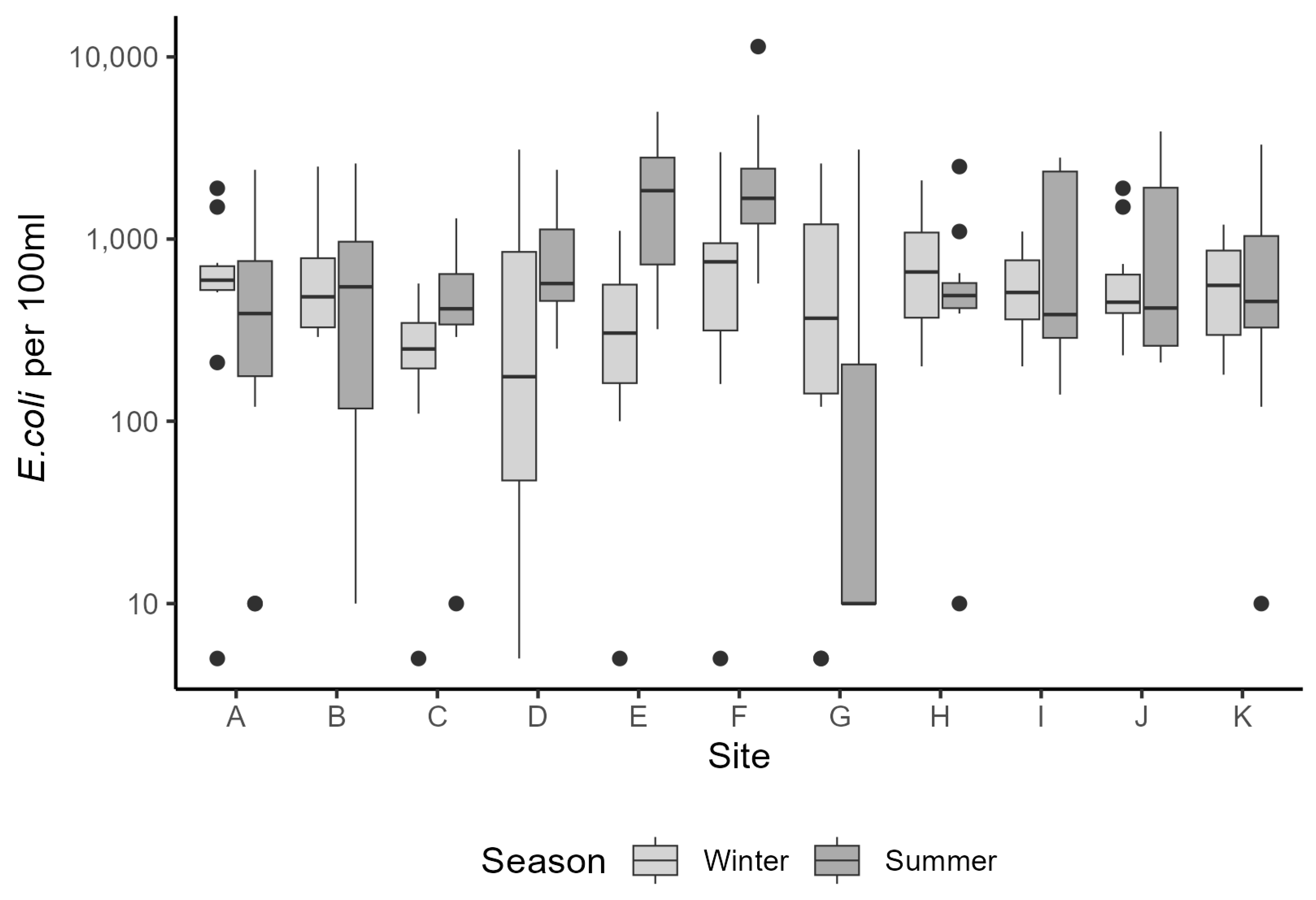
Each site was sampled 12 times per sampling period. The E. coli concentrations at each sampling site are presented for the winter and summer periods in Figure 3, and as winter and summer time series (see Supplementary Materials Figure SD1). E. coli concentrations were variable across sites and sampling periods, with between-site variability being more pronounced for the River Taw sites (A–G) than for the River Torridge sites (H–K). Winter median count was highest at Site F (750; interquartile range: 318 to 960) and lowest at Site D (180; interquartile range: 76 to 890), with considerable variation between sampling timepoints and a maximum count of 3100 at Site D at the first timepoint on 10 January 2023 (Figure SB1). Summer E. coli counts tended to be higher and more variable than winter counts. Median summer count was highest at Site E (1850; interquartile range: 738 to 2800) and lowest at Site G (10; interquartile range: 10 to 178), again with considerable variation between sampling timepoints and a maximum count of 11,400 at Site F on 20 June 2023.

Within the River Torridge catchment (excluding estuarine sites), there were 67 sample measurements for E. coli, at 10 separate sites, recorded in the 2023 Environment Agency (EA) Water Quality Data Archive (see Supplementary Materials Table SD2). Two sample measurements were recorded at each of these sites during the winter sampling period (January to March), but measurements were recorded at only 6 sites during the summer months (June to August); 5 of these had just 2 measurements and 1 site recorded only 1 measurement. Considering all measurements in 2023 for each of the Torridge EA monitoring sites, the mean E. coli concentration was 3202 cfu per 100 mL across all sites. This was influenced by 3 readings above 13,000 cfu per 100 mL, with a median value of 2257 cfu per 100 mL. Considering only measurements corresponding to the winter and summer sampling periods, the overall winter mean was 1771 cfu per 100 mL (ranging from 610 to 3580) and the summer mean was 1520 cfu per 100 mL (ranging from 665 to 2735). There were no corresponding data available for the Taw catchment.

3.2. SWAT Model Properties and Performance

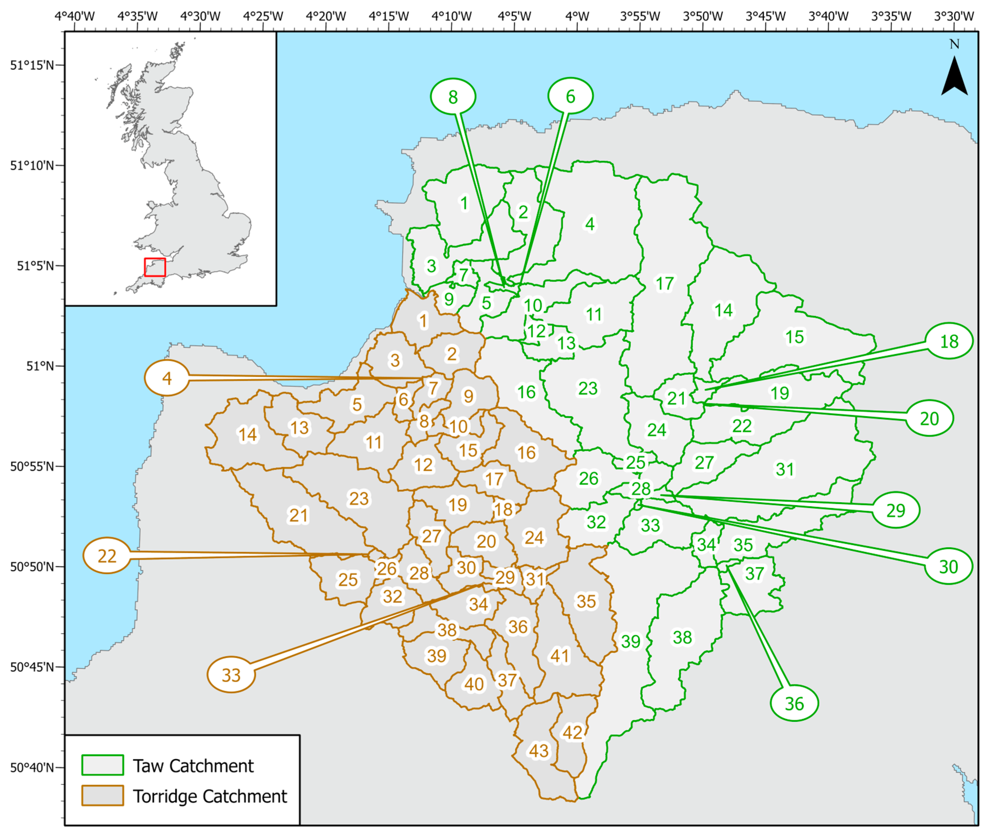
Watershed delineation by SWAT revealed the Taw to be the larger catchment, covering 122,367 ha compared with an area of 84,887 ha for the Torridge. However, the process produced more subbasins for the Torridge (43, versus 39 in the Taw), possibly reflecting a more complex stream network in this catchment. A map of the subbasins for each catchment is shown in Appendix A Figure A1.

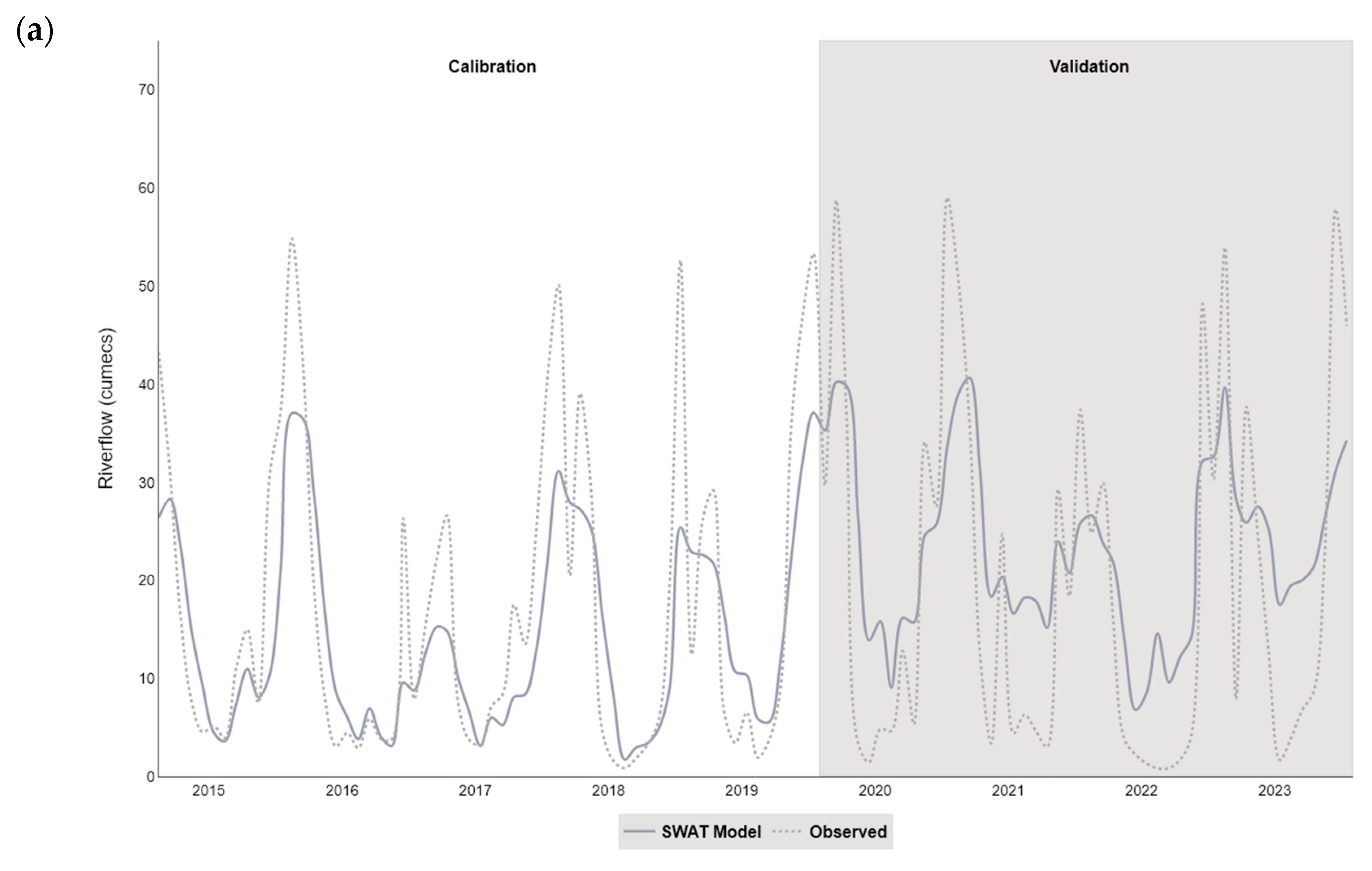
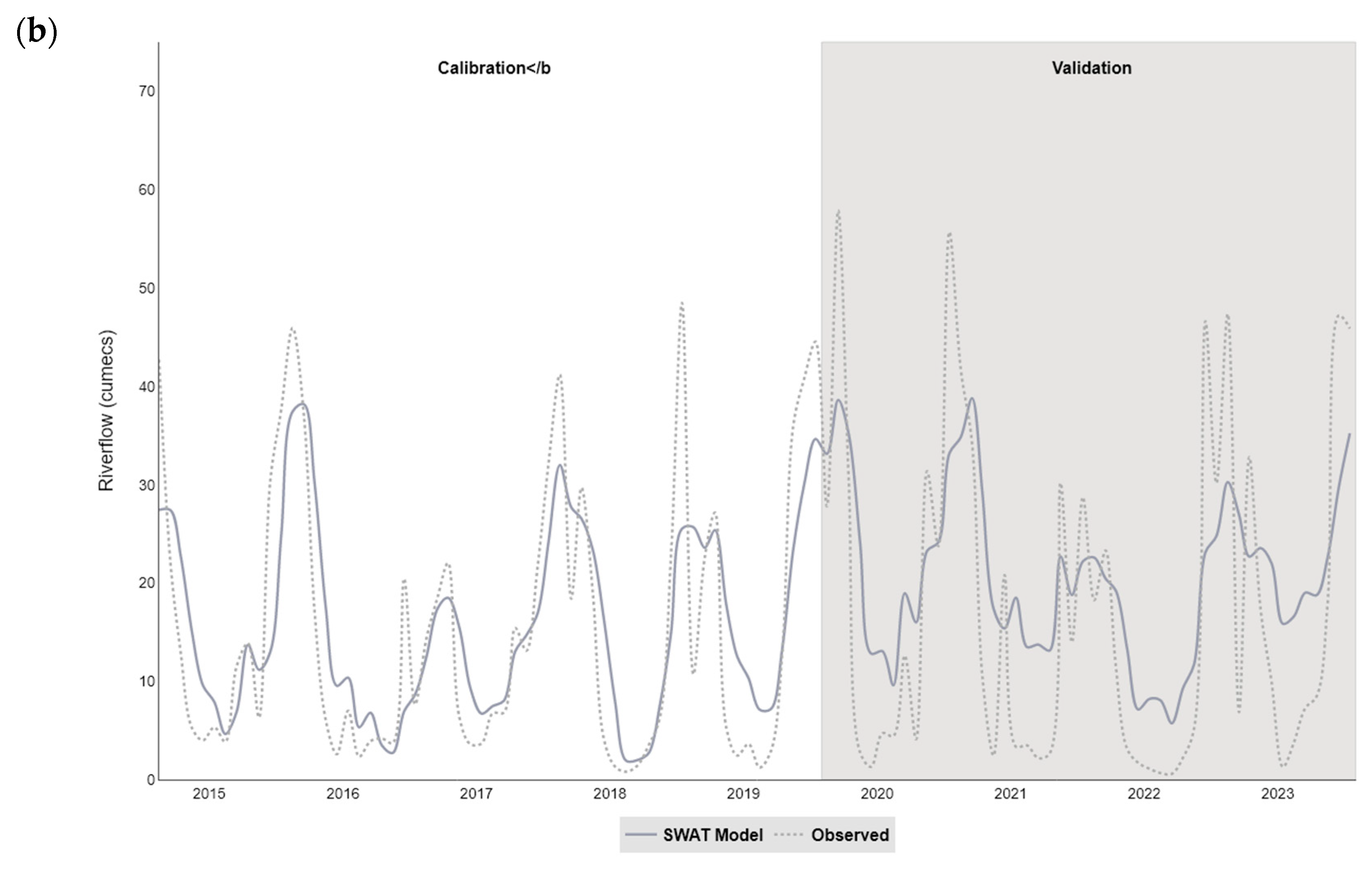
The initial SWAT models typically over-estimated riverine flows in the catchments and had low model efficacy. A subsequent sensitivity analysis performed on both models identified nine parameters with significant effect on catchment river flow. Using monthly river flow data, hard calibration was performed for model outputs between 01/01/2015 and 31/12/2019, and the best parameter values determined for each catchment model can be found in Supplementary Materials Table SC4, along with the performance characteristics of the SWAT models. Overall, based on objective functions, the Torridge model performed marginally better, with a Nash-Sutcliffe Efficiency (NSE) value of 0.65 versus 0.62 for the Taw (Kling-Gupta Efficiency (KGE) of 0.62 versus 0.58), and a Percent Bias (PBIAS) of 3.8 versus −12.5 when comparing monthly streamflow. According to the model efficiency classification of Moriasi et al. (2007) [55], the Torridge SWAT model was considered good, and the Taw SWAT model satisfactory. Model performance dipped slightly at the daily timestep, with an NSE of 0.47 for both the Taw and Torridge models. For the validation period 01/01/2020 to 31/12/2023, both models performed less well, with a drop in NSE values to 0.52 for the Taw and 0.49 for the Torridge (monthly streamflow). The reduction in performance, however, was less for the daily streamflow, dropping marginally to 0.36 for the Torridge and 0.41 for the Taw. For both models, the PBIAS increased for the validation period, suggesting an overestimation of streamflow in the validation period versus the calibration period. More details can be found in Appendix A 

Table A3. SWAT model performance.

Catchment	Time Frame	Objective Function	Calibration	Validation
Taw	Monthly	NSE	0.62	0.52
		KGE	0.57	0.42
		pBIAS	−12.5	21.1
	Daily	NSE	0.47	0.41
		KGE	0.45	0.35
		pBIAS	−12.5	20.9
Torridge	Monthly	NSE	0.65	0.49
		KGE	0.62	0.42
		pBIAS	3.8	22.3
	Daily	NSE	0.47	0.36
		KGE	0.46	0.32
		pBIAS	3.7	22.0

.

For both models there was a strong correlation between the observed and modelled streamflow at the river gauges (Pearson’s correlation coefficient of 0.79 and 0.68, for monthly and daily flows, respectively). Overall, the models were considered satisfactory, but typically underestimated flow during periods of high rainfall, and overestimated flow when rainfall was lower (see Figure 4 and Supplementary Materials Figure SC3). A similar pattern was reported by Coffey et al. 2010 [22] for catchments in Ireland. Furthermore, there was a small decrease in the efficacy of the models when considering daily rainfall.

3.3. Comparison of SWAT Outputs with Measured Values

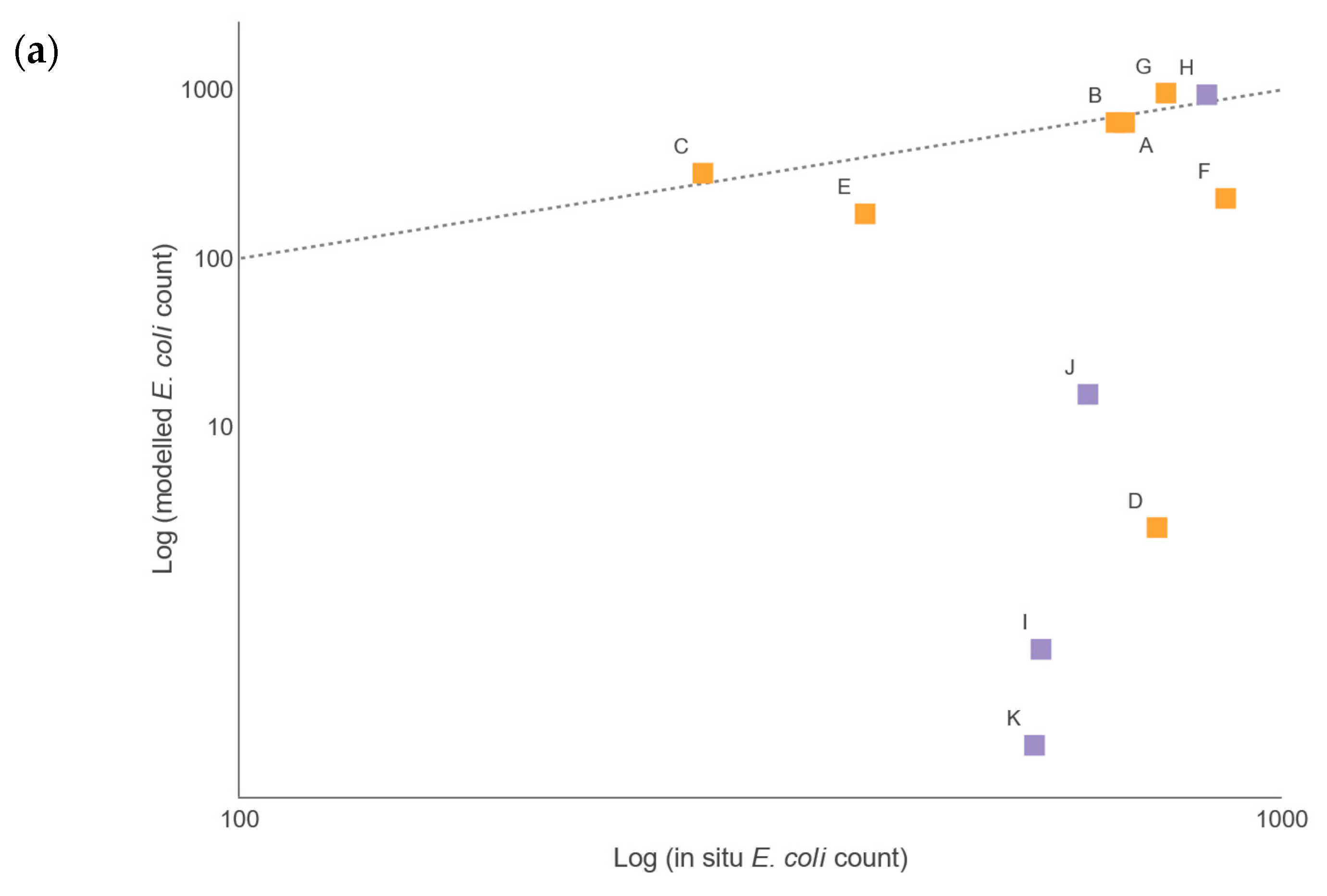
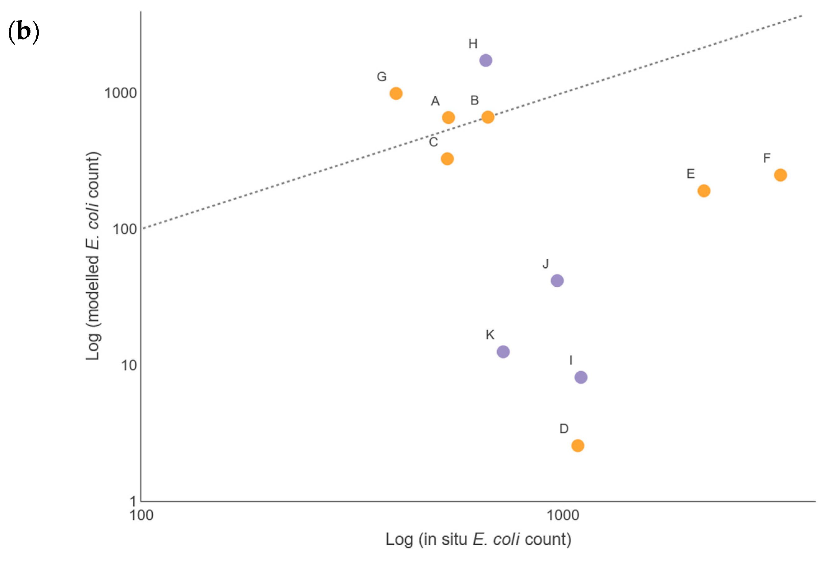
Simulated bacterial loads within the SWAT models were compared with the in situ measurements from the monitoring programme for the summer and winter periods. As SWAT results are based on concentrations, predictions tend to be high during low flow conditions and low for high flow conditions [22], and this pattern was observed in our study. Due to the variability in observation data, uncertainty in diffuse and point source bacterial inputs, and to facilitate comparison with other SWAT studies, the mean values of simulated versus observed loads at each site were calculated and plotted (Figure 5).

For the Taw catchment (orange symbols in Figure 5), Sites A, B, C, and G show reasonable agreement in the mean E. coli count for the summer and winter periods. Comparing mean values across the respective summer and winter seasons, Sites E and F are in reasonable agreement for the winter period, but less so in the summer period, when the SWAT model underestimates the E. coli count by an order of magnitude. Site D shows very poor agreement for both periods, with a very large underestimation of bacterial count by the model. The correlation between Sites A, B, C, G and H, which had mean modelled flow rates above 3 m³/s, was significant during the winter period (R² = 0.92, p < 0.05) but not during the summer, and correlation was poor when compared with the daily simulated output (see Supplementary Materials Table SE1). Conversely, sites with a low flow rate in summer and winter performed well in the summer period (R² = 0.96, p < 0.5) but poorly in the winter period (R² = 0.11, p > 0.05). Moreover, direct comparison of daily simulated output by NSE showed an efficiency of −0.47 for summer and −0.45 for winter. Individual site NSE values ranged from 0.11 to −1.97.

In the Torridge SWAT model, Sites I, J, and K (purple symbols in Figure 5) also show very poor agreement between the simulated bacterial counts and the observed site data for the summer and winter periods. Site H, however, shows reasonable agreement, better during the winter than the summer period. Furthermore, the Torridge SWAT model performed less well than the Taw model when comparing daily simulated bacterial loads with observed data. The overall NSE efficiency was −1.69 versus −0.47 for the winter and −1.13 versus −0.47 for the summer. Individual site NSE values from both models ranged from 0.15 to −5.22 (see Supplementary Materials Table SE2).

3.4. Influence of Spatial Distribution of Livestock on Predicted E. coli Loads

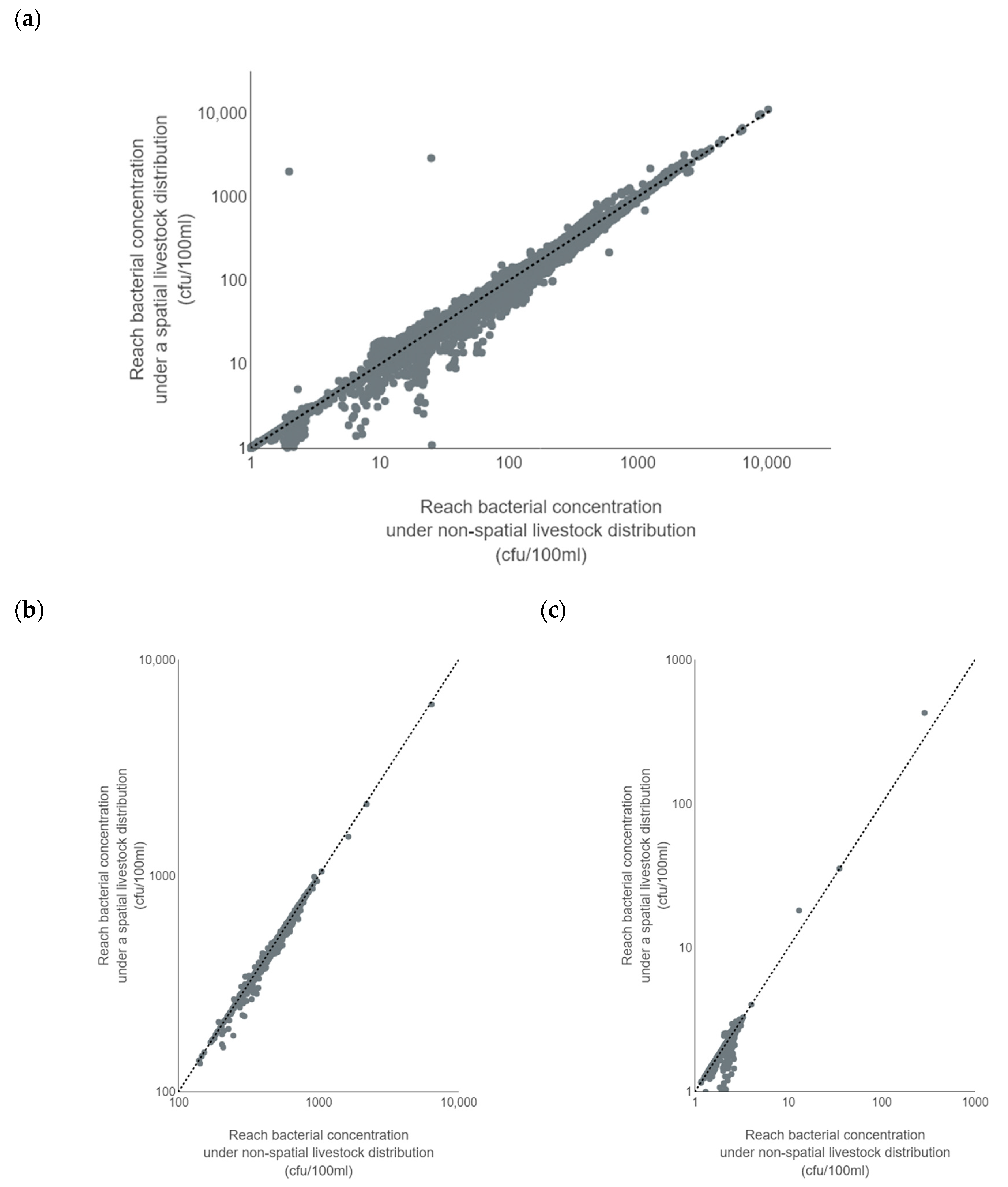
The transport and fate of E. coli in the catchments was modelled in SWAT using the pathogen module (see Materials and Methods for details), incorporating diffuse (agriculture) and point (discharges from WWTW and SOs) sources. Livestock represent a significant source of E. coli; therefore, the effect of distributing this source within specific subbasins of the SWAT models was investigated. The overall effect of spatial apportionment of livestock was to reduce the bacterial concentration in some reaches when the concentration was low (below 100 cfu/mL). This was balanced against more modest increases in most reaches, where concentrations were between 10 and 1000 cfu/mL (see Figure 6a and Supplementary Materials Figure SE1). The most significant effects were observed in those subbasins with a single outlet in the river channel network. Although the bacterial counts were generally lower in these reaches, the effect of spatial apportionment was more pronounced. For example, the reaches in subbasins 3, 19, 29, and 35 of the Taw catchment showed noticeable differences between the two approaches (see Appendix A Figure A1 for location of the subbasins). Spatial apportionment of livestock had a lesser influence on bacterial concentrations in those downstream river reaches associated with a larger number of upstream subbasins. This was especially true for those reaches closest to the outlet of the catchment, with greater differences seen in the upstream subbasins (for example, those reaches linked to subbasins 34, 36 and 38 in the Taw).

When considering the reaches associated with the water quality sample sites, there was little or no overall effect of spatial apportionment of livestock for Sites A, B, E, and K (see Supplementary Materials Figure SE2). Of course, some differences were evident due to specific daily conditions, but in general, a similar pattern of bacterial counts was observed. For Sites F, H, and J, the spatial apportionment resulted in an overall increase in modelled bacterial concentration in the reach, whereas an overall decrease was observed at Sites I, G, C, and D. These changes in livestock distribution did not account for the large differences between in situ measurements and model values for Sites D, I, J, and K (Figure 5), and presumably other factors caused this disparity. Only Site J showed an overall increase in concentration, but this was a mean increase of around 10%, with a maximum of 90%.

3.5. Statistical Analysis of Predictor Variables for Water Quality

Exploratory statistical analyses were carried out on winter and summer bacterial series from the 11 river sampling sites. Including site identification tended to improve the fit of generalized additive mixed models (GAMMs) for summer, but not the winter series (Supplementary Materials Figure SD1), suggesting more synchronicity in winter E. coli concentrations amongst the sites. Generally, the winter series were characterized by higher initial values followed by a large drop and then an increase toward the end of the sampling period, while the pattern was less clear in the summer series, with more inter-site variation and the presence of more extreme peaks (Supplementary Materials Figure SD2).

All time series across all sites and both sampling periods showed stationarity, indicating no overall trend in E. coli concentrations over time. Winter and summer site-specific series clustering sorted sites with similar features, but there was no evidence that sites clustered according to spatial distribution (Supplementary Materials Figure SD3), nor were these clusters static, with the clusters having different membership between seasons.

3.5.1. Linear Mixed-Effects Model Results

There was no evidence of temporal autocorrelation across both sampling periods, so no autocorrelation term was included in any of the LMMs. Winter LMMs were a poor fit to the data (R² < 0.15) and qualitatively worse than summer LMMs (R² > 0.35). While the best winter LMM included water temperature (positive coefficient) and cumulative 2-week rainfall (negative coefficient) as important variables, there was very little difference during model averaging in the fit of the top ranked models (

Table 3. Variable importance as sum of weights of linear mixed models, which contain each variable for each subset of data. Sum of weights > 0.6, indicated by shading, show most important variables within each subset of models.

Variable	Winter 1	Summer 1
temp	0.95 (0.91)	0.50 (0.47)
rain_2wk	0.92 (0.92)	0.28 (0.24)
PC1_proxi	0.42 (0.67)	0.36 (0.32)
PC1_subcatch	0.40 (0.36)	0.64 (0.46)
PC2_subcatch	0.35 (0.41)	0.62 (0.49)
PC1_immed	0.34 (0.33)	0.35 (0.32)
PC2_proxi	0.33 (0.40)	0.54 (0.68)
PC2_immed	0.30 (0.31)	0.47 (0.38)
rain_48	0.29 (0.28)	0.27 (0.28)
rain_24	0.27 (0.26)	0.99 (0.99)
min_distance	NA (0.64)	NA (0.53)

¹ Figures in brackets are with Site E excluded from the analysis. NA–Not Applicable

).

The best summer LMM included land use at the sub-catchment scale as a significant variable, with more arable land within the upstream sub-catchment resulting in higher E. coli counts. It also included cumulative 24-h rainfall (positive coefficient) as an important variable, but again there was very little difference during model averaging in the fit of the top ranked models.

3.5.2. Random Forest

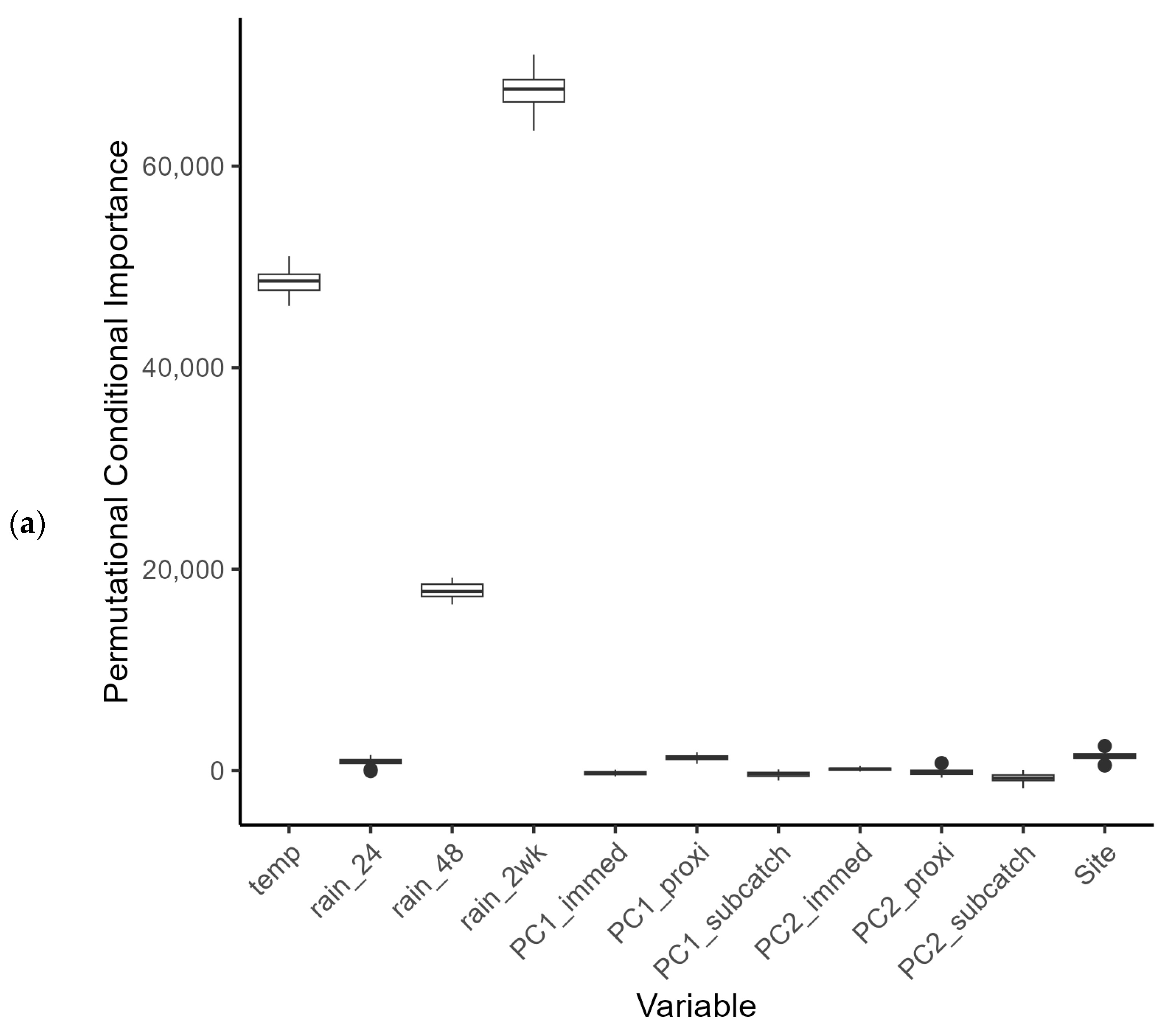
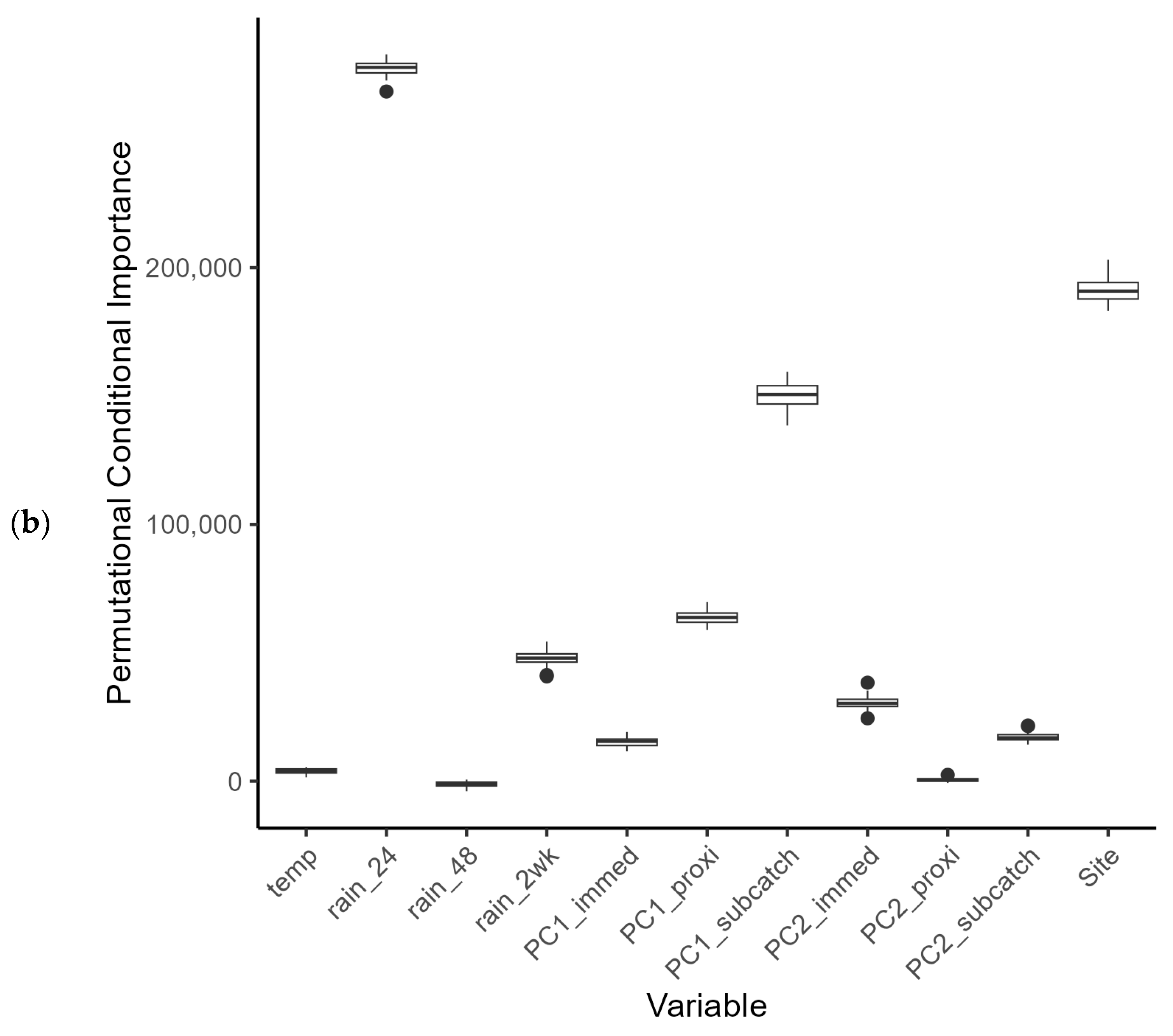
Random Forest regression produced qualitatively better fits to the winter data (R² > 0.26) and approximately equivalent fits to the summer (R² > 0.33) when compared to linear mixed models. This suggests that the flexibility of non-linear relationships is more suitable for characterizing winter data. For the winter random forest model, variable importance ranks the three highest variables as cumulative 2-week rainfall (overall negative relationship), water temperature (overall positive relationship), and cumulative 48-h rainfall (overall negative relationship) (Figure 7a). This agrees qualitatively with the LMM results.

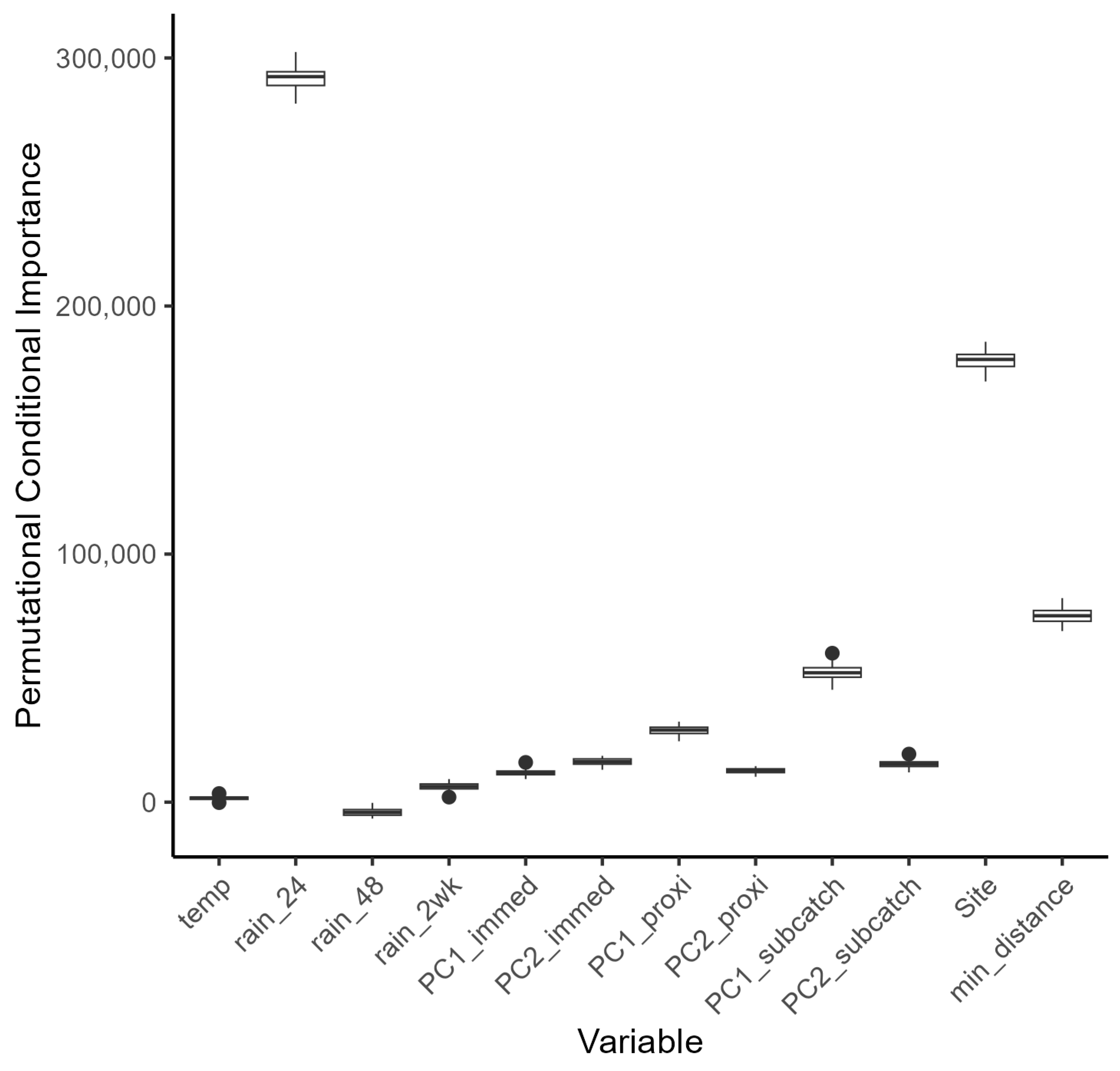
For the summer random forest model, variable importance ranks the three highest variables as cumulative 24-h rainfall (overall positive relationship), Site ID (consistent with the temporal patterns tested in the GAMM above), and sub-catchment land use (Figure 7b). This agrees with the summer LMM results. Subsetting the data, by omitting Site E (which had no upstream sewage point source in this data), results in minimum distance to point source emerging as the third most important variable in the summer forest model (Figure 8).

3.6. Rainfall Predictor Variables for Water Quality in the SWAT Models

Using the rainfall predictor variables identified in Section 3.5, exploratory statistical analyses were carried out using the subbasin rainfall and the bacterial loads for the 11 river sampling sites. As the SWAT model is a deterministic approach, generalized linear models were created for the summer and winter periods to attempt to describe the bacterial counts based on rainfall profiles (

Table 4. Generalized linear models for rainfall predictor variables for the bacterial loads at the water quality sites in the Taw and Torridge SWAT models with spatially distributed livestock numbers.

Model Coefficient Estimates	Winter	Summer
Intercept	1.59 **	1.05 **
Rainfall over the previous 24 h	0.025 NS	0.13 *
Rainfall over the previous 48 h	−0.006 NS	−0.053 NS
Rainfall over the previous 2 weeks	0.0033 **	0.0033 **

* p < 0.05; ** p < 0.01, ^NS–not significant.

). For both the summer and winter series, the linear models had low McFadden’s R² values (winter R² = 0.21; summer R² = 0.16), indicating that they were relatively poor predictors of the overall bacterial loads. This was in keeping with the modelling of the in situ data. Moreover, for the winter series, the only significant predictor variable was the rainfall over the previous 2 weeks, whereas for the summer series both the 24-h and 2-week rainfall variables were significant predictors of bacterial load. These findings were in close agreement with the in situ statistical data models. Care must be taken with these models because of the inherent collinearity between the rainfall variables.

4. Discussion

Ideally, a national water quality monitoring programme should adopt a mix of monitoring approaches underpinned by scientific reasoning, to ensure that all objectives are met for all necessary water quality metrics and to allow for readjustment in response to policy or other changes. Breaking down the various national monitoring programmes at the catchment level offers an approach to answering questions about best practice for water quality monitoring within riverine environments and providing actionable information for policy standards. Not only does this provide the opportunity to ensure the best monitoring approach for the resources available, but it also presents the opportunity to fill in monitoring gaps by using output from a validated model.

In our pilot study, Faecal Indicator Organism (FIO) data from the river water sampling were broadly in line with measured data from the national monitoring programme, albeit with higher E. coli counts overall. Both data sets were subject to large variation, with several very high readings above 13,000 counts (with a mean count of 3202 cfu per 100 mL). At present it is difficult to know whether these fluctuations are genuine spikes in bacterial load, or whether they represent a confounding effect during the sampling or measurement process (although the latter is unlikely, since standard protocols were used for sampling and analysis). Riverine bacterial loads did show a partial dependence on rainfall events within the catchments that was subtly different between the summer and winter periods (Challenge 1—see Introduction). Observational data for bacterial loads in watercourses can be highly variable (for example, see [22,56,57]) and in our study, variability was seen under the low flow regimen in summer and during peak flows in winter. This variation hampered statistical modelling based on catchment characteristics, but land use, more strictly land use within hydrological response units, was identified as a predictor variable for the summer period. Export of FIOs under dry and wet weather conditions has been shown to be associated with varying land use conditions [10], with improved pastureland identified as a primary control factor in catchments in Scotland [56]. During the UK summer, livestock are more likely to be outdoors, and those grazing in fields adjacent to watercourses are likely to add to the reservoir of faecal bacteria available to enter the river network [58]. According to UK government statistics, in 2023 69% of farm holdings always prevented livestock from entering watercourses, a percentage that has been rising since 2020 [37]. However, around 8% of farm holdings never prevented access, and this has remained relatively constant since 2020. It is well documented that quantities of faecal bacteria on fields, accumulated during long periods of dry weather, can be washed directly into watercourses by intense rainfall during subsequent summer storms, thereby causing large spikes in bacterial loadings [59]. This may be a contributing factor to the variation in bacterial loads during the summer in our catchments.

The catchment (SWAT) models developed in our study simulated the streamflow satisfactorily within the two catchments (NSE values of 0.62 for Taw and 0.65 for Torridge), and were more successful at modelling the monthly, rather than daily, time step. In particular, the models tended to overestimate flow during the summer months and underestimate flow in winter, a pattern that has been observed in studies using SWAT to model similar catchments (for example, see [16,22]). The SWAT 2012 architecture was superseded by SWAT+ [60], with more emphasis on spatial connectivity between features within the watershed. However, both models are limited in groundwater-driven watersheds, and a groundwater flow module is available for SWAT+ [61], which offers improvements to groundwater-surface water locations and rates, and nutrient loading via subsurface flow. Furthermore, the empirical curve number approach used in SWAT for rainfall-runoff simulation has recently come under scrutiny, and was outperformed by other methods for high-flow events [62]. The inability to faithfully simulate high rainfall-runoff events represents a major limitation for modelling faecal bacterial fate and transport from livestock in SWAT. Accounting for measured flow, even in a relatively small catchment, can be problematic due to uncertainties surrounding the contributions from field drains and other anthropogenic sources [57]. Whilst operation of SWAT at a sub-daily timestep appears to improve model efficiency for peak flows, this comes at a cost for medium flows, where the efficiency drops [63].

There were insufficient in situ observational data to validate our models for water quality assessment. In England, nutrient data (including nitrate, nitrite, ammonium, and ortho-phosphate) are collected monthly for many of the major rivers, but the collection points are rarely close to a river gauge, leading to greater inaccuracies in estimation of daily nutrient levels using flow rates. This hampers the creation and validation of accurate catchment models operating at a daily, or even sub-daily, time scale, a factor that is especially important with the increasing intensity of rainfall events in a changing climate. This has implications for modelling episodic bacterial contamination events that can occur under intense, short-duration rainfall events [10,56,64] affected by antecedent wetness [65], and was a severe limitation of the models developed in our study. Simulated bacterial counts at locations corresponding with the sampling sites showed reasonable levels of agreement for those rivers with good flow rates during the summer and winter periods. For example, the R² (Pearson) value for Sites A, B, C, and H was 0.64 and 0.95 for the respective summer and winter periods, when comparing the mean monthly simulated and observed bacterial loads. This comparison is often used to assess performance of SWAT models for bacterial load simulation (see [22,23,64]). However, when comparing the daily values directly, the correlation coefficient dropped to 0.03 for summer and 0.34 for winter, revealing the limitations of the model to operate faithfully at the daily level. Nevertheless, the modelled data responded to rainfall in the catchments in a similar manner, such that for the winter period, the 2-week rainfall pattern could be used in part as a predictor of the bacterial loads, and for the summer period the 24-h and, to some extent, the 2-week rainfall pattern, were significant predictors. This partially satisfies Challenge 3 (see Introduction), as it suggests that catchment modelling using SWAT has many of the routines needed to simulate the fate of bacteria in the watershed. Future work will consider the use of sub-daily rainfall in the SWAT models to improve the resolution; however, rainfall patterns alone did not produce a satisfactory model of bacterial output in the watercourses, and it was clear that rainfall was not the only predictor. For sites in low-flow regimens, the agreement between simulated and observed data was less good, with the model underestimating the bacterial load. Coffey et al. [22] observed a similar pattern for predictions of E. coli in Irish catchments, with best agreement between predicted and observed data found for moderate flow rates. Therefore, when modelling it is critically important to understand the flow rates and bacterial loads across many different parts of a catchment [57,66]. Often, calibration and validation of catchment models focuses on the watershed outlet, and this has come under criticism recently [62]. While this may seem intuitive, it exposes a major data gap for many regions and, while the model may show good agreement at the outlet, the upstream components may not reflect actual processes within the catchment. Recognition of this is important for policy advice and scenario testing and could be used to suggest sampling strategies to help fill the void.

Successful modelling of faecal coliforms within a catchment requires reliable information on the locations and loads for point source and diffuse inputs within a watershed. Implementation of diffuse source input from livestock can be problematic in the UK due to difficulties such as (1) obtaining precise numbers of animals for different livestock groups; (2) temporal and locational changes associated with the management of grazing livestock; (3) statistics only available for commercial farms; and (4) differences in livestock access to rivers, affecting the level of risk of faecal contamination. Livestock inputs are often incorporated into models by apportioning them evenly across a catchment as ‘average number of animals per hectare’ according to land use type (see, for example [22,23]). In this study, to investigate Challenge 2 (see Introduction), we explored spatial apportionment of livestock in the model that is more representative of their actual distribution within the catchment. A barrier to universal application of this approach is the limited availability of livestock data for small subsections of catchments (subbasins), or restrictions in areas where only a few farms are present for data protection and privacy concerns. This issue may become more pronounced with an increase in larger holdings in UK farming. In 2023, the average farm size was 69 ha for the southwest region of England, which includes the Taw and Torridge catchments [67]. This was the smallest average farm size for all regions in England, and 19 ha smaller than the average English farm. Despite this our study indicates that, for the smaller upstream subbasins within a catchment, better spatial apportionment of livestock can have a significant effect on bacterial input to the model.

In theory, inclusion of point sources in the catchment model should be relatively easy as their locations are often well known, as is the case for the UK, where point source locations of licenced discharges to watercourses (consented discharges) and SOs are readily available [39]. The major deficiency, however, is precise detail on what is being discharged, and when. For the consented continuous-treated effluent discharges, we used the dry weather flow as an estimate of daily discharge, but this assumes a steady discharge rate and does not account for discharges during wet flow conditions. Moreover, our model assumes that the spill pattern from SOs is related to rainfall within the catchment, although studies have suggested that SOs appear to spill more than the design criteria [68,69,70]. Furthermore, there are notable uncertainties around the actual effluent volumes and concentration of faecal bacteria within a given volume of discharge, and these are exacerbated for SO spills during heavy rainfall events, where the discharge may range from raw sewage to highly diluted effluent [71].

This study has highlighted some of the issues associated with setting up and refining models in data-limited situations. While modelling can assist with the estimation of water quality in unmonitored areas, the very existence of spatial and temporal gaps in established monitoring programmes creates challenges for model calibration and validation [72,73,74]. A potential solution to this problem is the deployment of remote sampling devices (sondes) to increase spatiotemporal density of sampling while minimizing manpower costs of sample collection and processing. However, to date, such devices have had issues regarding their reliability, calibration, and biofouling (see [75] for a review); therefore, siting them in optimal locations (for example, for ease of access, but without risk of vandalization) is key. Alternatively, a growing number of new initiatives involving citizen scientists (i.e., members of the public who volunteer to monitor and capture data in their locality) could help fill the gaps in formal monitoring programmes [76].

With increased complexities surrounding the nature and scale of inputs into UK rivers from land use and other activities, there is a need for further development of catchment models to assess and predict the likely impacts of future scenarios, not only on riverine water quality, but also on that of estuarine and coastal waters [64]. This paper has highlighted the challenges of creating a model representing the sources and pathways of faecal bacteria in a UK river catchment. In any such model there is considerable uncertainty in quantifying the bacterial input loads and spatial distribution of those inputs. This is especially pertinent when trying to assess the relationships between riverine loadings and intense rainfall events, for instance, which may produce wastewater spills or high volumes of run-off from the land, leading to potential shellfish hygiene issues and eutrophication of estuarine waters [64]. This type of assessment requires analysis at a daily, if not higher, temporal resolution, with the uncertainty of outputs increasing at finer spatial resolutions of the sub-catchment. While the model inputs could be refined with better data, such as improved spatial apportionment of livestock, due to current data limitations, validation of UK catchment models is almost always restricted to the drainage outlet. As well as preventing fine tuning of the model upstream and failing to properly account for processes in the upstream reaches, this could be a significant issue when considering the likely impacts of different scenarios, including the influence of climate change, on faecal contamination downstream.

5. Conclusions and Recommendations

In a resource-limited landscape, national-scale monitoring programmes for water quality tend to be both spatially and temporally sparse. Our study highlights seasonal differences in concentrations of monitored faecal bacteria, in part due to seasonal changes in rainfall. This suggests that risk-based monitoring, sufficient to capture possible seasonal trends, is key to ensuring water quality standards are met throughout the year. Another key finding was that spatial apportionment of livestock in the models had a modest effect on water quality outcomes at the drainage outlet, but was more important in the upstream reaches. This highlights the requirement to scrutinize monitoring observations in the context of the spatial spread of sampling sites. To elucidate, observations of good water quality within downstream catchment areas do not necessarily reflect the quality of water throughout the upstream sections. Finally, our study demonstrates the utility of catchment models for identifying data gaps and drawing attention to sub-catchment areas that may require better spatial targeting of monitoring efforts to underpin water quality improvement measures. Catchment models are often limited by a lack of suitable validation data, but the simulations they deliver, combined with robust statistical analyses such as those described here, can provide valuable insights to managers and policymakers to underpin robust monitoring strategies.

References

1. Grogan, A.E.; Mallin, M.A. Successful Mitigation of Stormwater-Driven Nutrient, Fecal Bacteria and Suspended Solids Loading in a Recreational Beach Community. J. Environ. Manag. 2021, 281, 111853. [Google Scholar] [CrossRef] [PubMed]
2. Hou, X.; Qin, L.; Wang, F.; Xu, M.; Yu, C.; Zhang, Y.; Zhang, T.; Wu, B.; Wang, D.; Li, M. Faecal Contamination in China: Trends, Sources, and Driving Mechanisms. Water Res. 2024, 261, 122017. [Google Scholar] [CrossRef] [PubMed]
3. Jeong, J.; Wagner, K.; Flores, J.J.; Cawthon, T.; Her, Y.; Osorio, J.; Yen, H. Linking Watershed Modeling and Bacterial Source Tracking to Better Assess E. coli Sources. Sci. Total Environ. 2019, 648, 164–175. [Google Scholar] [CrossRef] [PubMed]
4. Knöll, P.; Schiperski, F.; Roesrath, A.; Scheytt, T. Effects of Model Complexity on Karst Catchment Runoff Modeling for Flood Warning Systems. J. Hydrol. X 2025, 26, 100194. [Google Scholar] [CrossRef]
5. Ekanayaka, H.B.G.D.M.P.; Abeysingha, N.S.; Amarasekara, T.; Ray, R.L.; Samarathunga, D.K. The Use of InVEST-SDR Model to Evaluate Soil Erosion and Sedimentation in the Closer Catchment of a Proposed Tropical Reservoir in Sri Lanka. Int. J. Sediment Res. 2025, 40, 253–268. [Google Scholar] [CrossRef]
6. Nguyen, H.H.; Recknagel, F.; Meyer, W.; Frizenschaf, J.; Ying, H.; Gibbs, M.S. Comparison of the Alternative Models SOURCE and SWAT for Predicting Catchment Streamflow, Sediment and Nutrient Loads under the Effect of Land Use Changes. Sci. Total Environ. 2019, 662, 254–265. [Google Scholar] [CrossRef]
7. Ly, K.; Metternicht, G.; Marshall, L. Transboundary River Catchment Areas of Developing Countries: Potential and Limitations of Watershed Models for the Simulation of Sediment and Nutrient Loads. A Review. J. Hydrol. Reg. Stud. 2019, 24, 100605. [Google Scholar] [CrossRef]
8. Malham, S.K.; Taft, H.; Farkas, K.; Ladd, C.J.T.; Seymour, M.; Robins, P.E.; Jones, D.L.; McDonald, J.E.; Le Vay, L.; Jones, L. Multi-Scale Influences on Escherichia Coli Concentrations in Shellfish: From Catchment to Estuary. Environ. Pollut. 2025, 366, 125476. [Google Scholar] [CrossRef]
9. Neill, A.J.; Tetzlaff, D.; Strachan, N.J.C.; Hough, R.L.; Avery, L.M.; Watson, H.; Soulsby, C. Using Spatial-Stream-Network Models and Long-Term Data to Understand and Predict Dynamics of Faecal Contamination in a Mixed Land-Use Catchment. Sci. Total Environ. 2018, 612, 840–852. [Google Scholar] [CrossRef]
10. Kay, D.; Crowther, J.; Stapleton, C.M.; Wyer, M.D.; Fewtrell, L.; Anthony, S.; Bradford, M.; Edwards, A.; Francis, C.A.; Hopkins, M.; et al. Faecal Indicator Organism Concentrations and Catchment Export Coefficients in the UK. Water Res. 2008, 42, 2649–2661. [Google Scholar] [CrossRef]
11. Pathogen Surveillance in Agriculture, Food and Environment (PATH-SAFE) Programme | Food Standards Agency. Available online: https://www.food.gov.uk/our-work/pathogen-surveillance-in-agriculture-food-and-environment-path-safe-programme (accessed on 22 May 2025).
12. de Santana, C.O.; Spealman, P.; Gresham, D.; Dueker, M.E.; Perron, G.G. Bacterial and DNA Contamination of a Small Freshwater Waterway Used for Drinking Water after a Large Precipitation Event. Sci. Total Environ. 2025, 972, 179010. [Google Scholar] [CrossRef]
13. Lo, L.S.H.; Tong, R.M.K.; Chan, W.; Ho, W.; Cheng, J. Bacterial Pathogen Assemblages on Microplastic Biofilms in Coastal Waters. Mar. Pollut. Bull. 2025, 216, 117958. [Google Scholar] [CrossRef]
14. Posen, P.; Walker, D.; Cook, A.; Coyle, N.; Haverson, D.; Heal, R.; Hill, R.; Maskrey, B.; Rostant, W.; Ryder, D.; et al. Modelling Catchment-to-Coast Pathogen Transport in the Taw-Torridge: Report C8516-02 for PATH-SAFE. Cefas 2024, C8516–02, 181. [Google Scholar]
15. Arnold, J.G.; Srinivasan, R.; Muttiah, R.S.; Williams, J.R. Large Area Hydrologic Modeling and Assessment Part I: Model Development. J. Am. Water Resour. Assoc. 1998, 34, 73–89. [Google Scholar] [CrossRef]
16. Holder, A.J.; Rowe, R.; McNamara, N.P.; Donnison, I.S.; McCalmont, J.P. Soil & Water Assessment Tool (SWAT) Simulated Hydrological Impacts of Land Use Change from Temperate Grassland to Energy Crops: A Case Study in Western UK. GCB Bioenergy 2019, 11, 1298–1317. [Google Scholar] [CrossRef]
17. Tuladhar, A.; Bailey, R.T.; Abbas, S.A.; Shanmugam, M.S.; Arnold, J.G.; White, M.J. Quantifying the Impact of Climate Change and Land Use Change on Surface-Subsurface Nutrient Dynamics in a Chesapeake Bay Watershed System. J. Environ. Manag. 2025, 380, 125101. [Google Scholar] [CrossRef] [PubMed]
18. Haque, M.H.; Ansari, A.H.; Veith, T.L.; White, M.J.; Costello, C.; Spiegal, S.; Kleinman, P.J.A.; Arnold, J.G.; Cibin, R. Reducing National Water Degradation: Development and Application of a Manureshed-Identification Framework. Agric. Syst. 2025, 227, 104349. [Google Scholar] [CrossRef]
19. Grosser, P.F.; Schmalz, B. Assessing the Impacts of Climate Change on Hydrological Processes in a German Low Mountain Range Basin: Modelling Future Water Availability, Low Flows and Water Temperatures Using SWAT+. Environments 2025, 12, 151. [Google Scholar] [CrossRef]
20. Szalińska, E.; Motyka, J.; d’Obyrn, K.; Orlińska-Woźniak, P.; Nachlik, E.; Mączałowski, A.; Wilk, P. Current and Future Chloride Concentrations in a Large River—Will a Disaster Happen Again? Water Resour. Ind. 2025, 33, 100289. [Google Scholar] [CrossRef]
21. Bailey, R.T.; Tavakoli-Kivi, S.; Wei, X. A Salinity Module for SWAT to Simulate Salt Ion Fate and Transport at the Watershed Scale. Hydrol. Earth Syst. Sci. 2019, 23, 3155–3174. [Google Scholar] [CrossRef]
22. Coffey, R.; Cummins, E.; Bhreathnach, N.; Flaherty, V.O.; Cormican, M. Development of a Pathogen Transport Model for Irish Catchments Using SWAT. Agric. Water Manag. 2010, 97, 101–111. [Google Scholar] [CrossRef]
23. Coffey, R.; Dorai-Raj, S.; O’Flaherty, V.; Cormican, M.; Cummins, E. Modeling of Pathogen Indicator Organisms in a Small-Scale Agricultural Catchment Using SWAT. Hum. Ecol. Risk Assess. Int. J. 2013, 19, 232–253. [Google Scholar] [CrossRef]
24. South West England’s Regional Climate. Available online: https://www.metoffice.gov.uk/binaries/content/assets/metofficegovuk/pdf/weather/learn-about/weather/regional-climates/south-west-england_-climate-met-office.pdf (accessed on 16 June 2025).
25. FSA. Protocol for Sampling and Transport of Water Samples for the Purpose of Official Control Monitoring of Classified Shellfish Production Areas Under Commission Implementing Regulation (EU) 2019/627. Food Standards Agency. 2020. Available online: https://www.food.gov.uk/sites/default/files/media/document/sampling-protocol-water-samples-july-2020.pdf (accessed on 18 July 2025).
26. ESRI ArcGIS Desktop, version 10.5; Esri: Mumbai, India, 2024.
27. Environment Agency LIDAR Composite DTM 2019–10m. Available online: https://www.data.gov.uk/dataset/8311f42d-bddd-4cd4-98a3-e543de5be4cb/lidar-composite-dtm-2019-10m (accessed on 3 June 2025).
28. EA Detailed River Network (DRN). Available online: https://catalogue.ceh.ac.uk/id/6071dc92-008f-41e3-a4fa-bb039c771c9b (accessed on 3 June 2025).
29. European Environment Agency CORINE Land Cover 2018 (Raster 100 m), Europe, 6-Yearly—Version 2020_20u1, May 2020. Available online: https://sdi.eea.europa.eu/catalogue/copernicus/api/records/960998c1-1870-4e82-8051-6485205ebbac?language=all (accessed on 3 June 2025).
30. FAO/UNESCO Soil Map of the World | FAO SOILS PORTAL | Food and Agriculture Organization of the United Nations. Available online: https://www.fao.org/soils-portal/data-hub/soil-maps-and-databases/faounesco-soil-map-of-the-world/en/ (accessed on 3 June 2025).
31. Legg, T.; Packman, S.; Caton Harrison, T.; McCarthy, M. An Update to the Central England Temperature Series—HadCET v2.1. Geosci. Data J. 2025, 12, e284. [Google Scholar] [CrossRef]
32. Open WIMS Data. Available online: https://environment.data.gov.uk/water-quality/view/landing (accessed on 3 June 2025).
33. R Core Team. R: A Language and Environment for Statistical Computing; The R Foundation for Statistical Computing: Vienna, Austria, 2022. [Google Scholar]
34. Nguyen, T.V.; Dietrich, J.; Dang, T.D.; Tran, D.A.; Van Doan, B.; Sarrazin, F.J.; Abbaspour, K.; Srinivasan, R. An Interactive Graphical Interface Tool for Parameter Calibration, Sensitivity Analysis, Uncertainty Analysis, and Visualization for the Soil and Water Assessment Tool. Environ. Model. Softw. 2022, 156, 105497. [Google Scholar] [CrossRef]
35. Gupta, H.V.; Kling, H. On Typical Range, Sensitivity, and Normalization of Mean Squared Error and Nash-Sutcliffe Efficiency Type Metrics. Water Resour. Res. 2011, 47, 2011WR010962. [Google Scholar] [CrossRef]
36. UK National River Flow Archive Dataset. 2025. Available online: https://nrfa.ceh.ac.uk/nrfa-publications/nrfa-scientific-publications (accessed on 16 June 2025).
37. Farming Statistics—Land Use, Livestock Populations and Agricultural Workforce as at 1 June 2021, England. Available online: https://www.gov.uk/government/statistics/farming-statistics-land-use-livestock-populations-and-agricultural-workforce-as-at-1-june-2021-england (accessed on 3 June 2025).
38. Sowah, R.A.; Bradshaw, K.; Snyder, B.; Spidle, D.; Molina, M. Evaluation of the Soil and Water Assessment Tool (SWAT) for Simulating E. coli Concentrations at the Watershed-Scale. Sci. Total Environ. 2020, 746, 140669. [Google Scholar] [CrossRef]
39. Consented Discharges to Controlled Waters with Conditions. Available online: https://www.data.gov.uk/dataset/55b8eaa8-60df-48a8-929a-060891b7a109/consented-discharges-to-controlled-waters-with-conditions1 (accessed on 3 January 2024).
40. Environment Agency Event Duration Monitoring—Storm Overflows—Annual Returns 2023. Available online: https://environment.data.gov.uk/dataset/21e15f12-0df8-4bfc-b763-45226c16a8ac (accessed on 3 January 2024).
41. Met Office MIDAS Open: UK Daily Weather Observation Data, V202407. Available online: https://catalogue.ceda.ac.uk/uuid/8070d47e1b7340468fa7cf654dee938b (accessed on 3 June 2025).
42. García-García, L.M.; Campos, C.J.A.; Kershaw, S.; Younger, A.; Bacon, J. Scenarios of Intermittent E. coli Contamination from Sewer Overflows to Shellfish Growing Waters: The Dart Estuary Case Study. Mar. Pollut. Bull. 2021, 167, 112332. [Google Scholar] [CrossRef]
43. Wood, S.N. Fast Stable Restricted Maximum Likelihood and Marginal Likelihood Estimation of Semiparametric Generalized Linear Models. J. R. Stat. Soc. Ser. B Stat. Methodol. 2011, 73, 3–36. [Google Scholar] [CrossRef]
44. Wood, S.N. Thin Plate Regression Splines. J. R. Stat. Soc. Ser. B Stat. Methodol. 2003, 65, 95–114. [Google Scholar] [CrossRef]
45. Sardá-Espinosa, A. Time-Series Clustering in R Using the Dtwclust Package. R J. 2019, 11, 22–43. [Google Scholar] [CrossRef]
46. Kwiatkowski, D.; Phillips, P.C.B.; Schmidt, P.; Shin, Y. Testing the Null Hypothesis of Stationarity against the Alternative of a Unit Root: How Sure Are We That Economic Time Series Have a Unit Root? J. Econom. 1992, 54, 159–178. [Google Scholar] [CrossRef]
47. O’Hara-Wild, M.; Hyndman, R.; Wang, E. Feasts: Feature Extraction and Statistics for Time Series. Available online: https://CRAN.R-project.org/package=feasts (accessed on 3 June 2025).
48. Hyndman, R.; Athanasopoulos, G. Forecasting: Principles and Practice, 2nd ed.; OTexts: Sydney, Australia, 2018. [Google Scholar]
49. Pinheiro, J.; Bates, D. Nlme: Linear and Nonlinear Mixed Effects Models; R Core Team: Vienna, Austria, 2022. [Google Scholar]
50. Bartoń, K. MuMIn: Multi-Model Inference. Available online: https://cran.r-project.org/web/packages/MuMIn/index.html (accessed on 3 June 2025).
51. Burnham, K.P.; Anderson, D.R. (Eds.) Model Selection and Multimodel Inference; Springer: New York, NY, USA, 2004; ISBN 978-0-387-95364-9. [Google Scholar]
52. Strobl, C.; Boulesteix, A.-L.; Kneib, T.; Augustin, T.; Zeileis, A. Conditional Variable Importance for Random Forests. BMC Bioinform. 2008, 9, 307. [Google Scholar] [CrossRef]
53. Hothorn, T.; Kurt, H.; Zeileis, A. Unbiased Recursive Partitioning: A Conditional Inference Framework. J. Comput. Graph. Stat. 2006, 15, 651–674. [Google Scholar] [CrossRef]
54. Strobl, C.; Boulesteix, A.-L.; Zeileis, A.; Hothorn, T. Bias in Random Forest Variable Importance Measures: Illustrations, Sources and a Solution. BMC Bioinform. 2007, 8, 25. [Google Scholar] [CrossRef]
55. Moriasi, D.N.; Arnold, J.G.; Van Liew, M.W.; Bingner, R.L.; Harmel, R.D.; Veith, T.L. Model Evaluation Guidelines for Systematic Quantification of Accuracy in Watershed Simulations. Trans. ASABE 2007, 50, 885–900. [Google Scholar] [CrossRef]
56. Tetzlaff, D.; Capell, R.; Soulsby, C. Land Use and Hydroclimatic Influences on Faecal Indicator Organisms in Two Large Scottish Catchments: Towards Land Use-Based Models as Screening Tools. Sci. Total Environ. 2012, 434, 110–122. [Google Scholar] [CrossRef] [PubMed]
57. Edwards, A.C.; Watson, H.A.; Cook, Y.E.M. Source Strengths, Transport Pathways and Delivery Mechanisms of Nutrients, Suspended Solids and Coliforms within a Small Agricultural Headwater Catchment. Sci. Total Environ. 2012, 434, 123–129. [Google Scholar] [CrossRef]
58. Fisher, D.S.; Steiner, J.L.; Endale, D.M.; Stuedemann, J.A.; Schomberg, H.H.; Franzluebbers, A.J.; Wilkinson, S.R. The Relationship of Land Use Practices to Surface Water Quality in the Upper Oconee Watershed of Georgia. For. Ecol. Manag. 2000, 128, 39–48. [Google Scholar] [CrossRef]
59. Soulsby, C.; Petry, J.; Brewer, M.J.; Dunn, S.M.; Ott, B.; Malcolm, I.A. Identifying and Assessing Uncertainty in Hydrological Pathways: A Novel Approach to End Member Mixing in a Scottish Agricultural Catchment. J. Hydrol. 2003, 274, 109–128. [Google Scholar] [CrossRef]
60. Bieger, K.; Arnold, J.G.; Rathjens, H.; White, M.J.; Bosch, D.D.; Allen, P.M.; Volk, M.; Srinivasan, R. Introduction to SWAT+, A Completely Restructured Version of the Soil and Water Assessment Tool. J. Am. Water Resour. Assoc. 2017, 53, 115–130. [Google Scholar] [CrossRef]
61. Bailey, R.T.; Bieger, K.; Arnold, J.G.; Bosch, D.D. A New Physically-Based Spatially-Distributed Groundwater Flow Module for SWAT+. Hydrology 2020, 7, 75. [Google Scholar] [CrossRef]
62. Tasdighi, A.; Arabi, M.; Harmel, D. A Probabilistic Appraisal of Rainfall-Runoff Modeling Approaches within SWAT in Mixed Land Use Watersheds. J. Hydrol. 2018, 564, 476–489. [Google Scholar] [CrossRef]
63. Brighenti, T.M.; Bonumá, N.B.; Srinivasan, R.; Chaffe, P.L.B. Simulating Sub-Daily Hydrological Process with SWAT: A Review. Hydrol. Sci. J. 2019, 64, 1415–1423. [Google Scholar] [CrossRef]
64. Ferreira, J.G.; Bernard-Jannin, L.; Cubillo, A.; Lencart, E.; Silva, J.; Diedericks, G.P.J.; Moore, H.; Service, M.; Nunes, J.P. From Soil to Sea: An Ecological Modelling Framework for Sustainable Aquaculture. Aquaculture 2023, 577, 739920. [Google Scholar] [CrossRef]
65. Wallace, S.; Biggs, T.; Lai, C.-T.; McMillan, H. Tracing Sources of Stormflow and Groundwater Recharge in an Urban, Semi-Arid Watershed Using Stable Isotopes. J. Hydrol. Reg. Stud. 2021, 34, 100806. [Google Scholar] [CrossRef]
66. Snelder, T.; Elliott, S.; Muirhead, R.; Fraser, C. Parameters for Simple Empirical Catchment Water Quality Models for Simulating Escherichia coli in New Zealand Rivers; AgResearch: Palmerston North, New Zealand, 2024. [Google Scholar]
67. Agricultural Facts: South West Region. Available online: https://www.gov.uk/government/statistics/agricultural-facts-england-regional-profiles/agricultural-facts-south-west-region (accessed on 3 June 2025).
68. Younger, A.; Kershaw, S.; Campos, C.J.A. Performance of Storm Overflows Impacting on Shellfish Waters in England. Land 2022, 11, 1576. [Google Scholar] [CrossRef]
69. Hammond, P.; Suttie, M.; Lewis, V.T.; Smith, A.P.; Singer, A.C. Detection of Untreated Sewage Discharges to Watercourses Using Machine Learning. npj Clean Water 2021, 4, 18. [Google Scholar] [CrossRef]
70. Giakoumis, T.; Voulvoulis, N. Water Framework Directive Programmes of Measures: Lessons from the 1st Planning Cycle of a Catchment in England. Sci. Total Environ. 2019, 668, 903–916. [Google Scholar] [CrossRef]
71. Petrie, B. A Review of Combined Sewer Overflows as a Source of Wastewater-Derived Emerging Contaminants in the Environment and Their Management. Environ. Sci. Pollut. Res. 2021, 28, 32095–32110. [Google Scholar] [CrossRef] [PubMed]
72. Nyeko, M. Hydrologic Modelling of Data Scarce Basin with SWAT Model: Capabilities and Limitations. Water Resour. Manag. 2015, 29, 81–94. [Google Scholar] [CrossRef]
73. Murumkar, A.; Tapas, M.; Martin, J.; Kalcic, M.; Shedekar, V.; Goering, D.; Thorstensen, A.; Boles, C.; Redder, T.; Confesor, R. Advancing SWAT Modeling with Rainfall Risk-Based Fertilizer Timing to Improve Nutrient Management and Crop Yields. Agric. Water Manag. 2025, 316, 109555. [Google Scholar] [CrossRef]
74. Rasheed, N.J.; Al-Khafaji, M.S.; Alwan, I.A.; Al-Suwaiyan, M.S.; Doost, Z.H.; Yaseen, Z.M. Survey on the Resolution and Accuracy of Input Data Validity for SWAT-Based Hydrological Models. Heliyon 2024, 10, e38348. [Google Scholar] [CrossRef]
75. Lal, K.; Jaywant, S.A.; Arif, K.M. Electrochemical and Optical Sensors for Real-Time Detection of Nitrate in Water. Sensors 2023, 23, 7099. [Google Scholar] [CrossRef] [PubMed]
76. Quinlivan, L.; Chapman, D.V.; Sullivan, T. Validating Citizen Science Monitoring of Ambient Water Quality for the United Nations Sustainable Development Goals. Sci. Total Environ. 2020, 699, 134255. [Google Scholar] [CrossRef] [PubMed]
Figure 1. Study area in the lower catchment area of the Rivers Taw and Torridge in north Devon, UK, showing the main wastewater treatment works, river water sampling locations used for the study, and the estuarine shellfish harvesting area.
Hydrology 12 00212 g001
Figure 2. Cattle density in the subbasins of the Taw and Torridge catchments in 2021. Average cattle density for the Taw catchment was 1.23 LU ha−1 and for the Torridge was 2.51 LU ha−1. Orange symbols represent variable livestock density in the Taw catchment (white background), whereas green symbols represent variable livestock in the Torridge catchment (mid grey background). Dark grey livestock symbols indicate subbasins where the average livestock density values were assigned. For the equivalent spatial distribution for sheep, see Supplementary Materials Figure SC1.
Hydrology 12 00212 g002
Figure 3. Boxplot of E. coli concentrations (cfu/100 mL) found at 11 river sampling sites (see Figure 1 for locations of sites A–K) during winter (light grey boxes) and summer (dark-grey boxes) sampling periods. Boxes show median and interquartile range; whiskers show 1.5 × interquartile range.
Hydrology 12 00212 g003
Figure 4. (a) Comparison of the simulated monthly streamflow from the Taw SWAT model with observed river flows for the river gauge at Umberleigh. (b) Comparison of the simulated monthly streamflow from the Torridge SWAT model with observed river flows for the river gauge at Torrington.
Hydrology 12 00212 g004aHydrology 12 00212 g004b
Figure 5. Comparison between simulated (monthly) bacterial counts estimated by the SWAT models and observed bacterial counts measured at the respective Taw (orange) and Torridge (purple) sample sites (see Figure 1 for locations of sites A–K): (a) winter; (b) summer. The reference line (dotted) indicates when the modelled and in situ values are identical.
Hydrology 12 00212 g005aHydrology 12 00212 g005b
Figure 6. Comparisons between simulated bacterial loads arising from spatial versus non-spatial apportionment of livestock in the catchment model: (a) across all river reaches in the Taw SWAT model; (b) at Site A; (c) at Site D. The reference line (dotted) indicates when the modelled and in situ values are identical.
Hydrology 12 00212 g006
Figure 7. Variable importance for all sites from conditional random forest models: (a) winter; (b) summer. Permutational conditional importance used with fifty replicates.
Hydrology 12 00212 g007aHydrology 12 00212 g007b
Figure 8. Summer variable importance for subset of sites from conditional random forest model. Permutational conditional importance used with fifty replicates. Note that subsetting data (by omitting Site E) results in minimum distance to point source emerging as third most important variable.
Hydrology 12 00212 g008