Review

Half-Century Review and Advances in Closed-Form Functions for Estimating Soil Water Retention Curves

by
Ali Rasoulzadeh
1,
Javad Bezaatpour
2,
Javanshir Azizi Mobaser
1 and
Jesús Fernández-Gálvez
3,*
1
Water Engineering Department, Faculty of Agriculture and Natural Resources, University of Mohaghegh Ardabili, Ardabil 56199-11367, Iran
2
Environmental Engineering Research Center, Chemical Engineering Department, Sahand University of Technology, Sahand New Town, Tabriz 51335-1996, Iran
3
Department of Regional Geographic Analysis and Physical Geography, University of Granada, 18011 Granada, Spain
*
Author to whom correspondence should be addressed.
Hydrology 2025, 12(7), 164; https://doi.org/10.3390/hydrology12070164
Submission received: 14 May 2025 / Revised: 11 June 2025 / Accepted: 13 June 2025 / Published: 25 June 2025

Abstract

This review provides a comprehensive overview of the closed-form expressions developed for estimating the soil water retention curve (SWRC) from 1964 to the present. Since the concept of the SWRC was introduced in 1907, numerous closed-form functions have been proposed to describe the relationship between soil matric suction and volumetric water content, each with distinct strengths and limitations. Given the variability in SWRC shapes influenced by soil texture, structure, and organic matter, models in the form of sigmoidal, multi-exponential, lognormal, hyperbolic, and hybrid functions have been designed to fit experimental SWRC data. Based on the number of adjustable parameters, these models are categorized into three main groups: three-, four-, and five-parameter models. They can also be classified as one-, two-, or three-segment functions depending on their structural complexity. A review of the developed models indicates that most are effective in representing the SWRC between the residual and saturated water content range. To capture the full range of the SWRC, hybrid functions have been proposed by combining traditional models. This review presents and discusses these models in chronological order of publication.

1. Introduction

The soil water retention curve (SWRC) is a fundamental hydraulic characteristic used to quantify and simulate water and contaminant movement in the vadose zone. Computer software and source codes commonly employed in soil and water sciences are built using SWRC equations. These predictive models, expressed as differentiable functions, are used alongside hydraulic conductivity (HC) curves to describe water flow by solving the Richards equation [1] through numerical methods, such as finite difference or finite element approaches.
SWRC and HC functions are classified as hard-to-measure soil hydraulic properties due to the complex nature of soil media [2,3]. In soil and water sciences, both direct (laboratory-based) and indirect (predictive mathematical or conceptual models) methods are used to characterize the SWRC [4,5]. Despite significant advances in measurement techniques, direct methods remain time-consuming, labor-intensive, and costly, requiring high technical expertise [6,7,8,9,10]. Additionally, SWRC measurements are typically performed on small undisturbed or disturbed soil samples in the laboratory or via small-scale in situ tests [11].
Laboratory tests for SWRC determination generally use porous media-based methods, such as sandbox experiments, hanging water columns, pressure cells, pressure plate extractors, and centrifuges [12,13,14,15]. In contrast, in situ tests commonly utilize tension disc infiltrometers, gamma-ray attenuation, ground-penetrating radar, and soil water content probes [5,7,16,17,18].
Given these limitations, indirect methods have gained considerable attention as viable alternatives. These methods are grouped into three main categories: physical–empirical models [6,19,20,21,22], pedotransfer functions (PTFs) [23,24,25], and fractal models [26,27,28,29,30]. These methods estimate the SWR and HC curves by establishing significant relationships between readily measurable soil properties (e.g., texture, particle size distribution, bulk density, and organic matter) and properties that are difficult to measure directly are estimated.
Closed-form expressions have been widely used by researchers and modelers to predict SWRC behavior for several important reasons [31]. First, they provide analytical equations that describe the relationship between effective saturation, hydraulic conductivity, and pressure head. Second, closed-form expressions can easily accommodate inverse calculation methods, enabling the evaluation of model performance by fitting results to experimental data using iterative algorithms. Additionally, model parameters can be experimentally calibrated for various soil types [32,33,34]. Analytical expressions also facilitate rapid parametric comparisons of hydraulic properties across different soil types, making it possible to investigate how changes in model parameters affect the shape of the SWRC.
The SWRC typically exhibits an S-shaped curve due to the curvature change at the inflection point, which can only be captured by specific types of mathematical expressions. Since laboratory measurements typically focus on the drying branch of the SWRC, most proposed models are derived from empirical data corresponding to this branch.
Although there has been relatively limited development of fundamentally new SWRC models in recent decades, summarizing and systematically analyzing existing models remains highly relevant. Many of these models are still widely used in hydrology, soil physics, and environmental engineering, and model selection can significantly influence simulation results and practical decisions. Furthermore, advances in data availability, parameter estimation techniques, and computational tools have renewed interest in applying and comparing established SWRC models under a wider range of conditions. This review therefore aims to provide an updated and structured overview of the main SWRC models, highlighting their respective strengths, limitations, and areas of applicability, to support both researchers and practitioners in the field.
This paper provides a comprehensive overview of SWRC models, organized chronologically by their publication date, and evaluates their strengths and limitations. In addition to analyzing model performance, this review examines how well different models fit laboratory-measured SWRC data. To illustrate model fitting, the SWRCs of a fine-textured (clay) soil and a coarse-textured (loamy sand) soil are used as representative samples. The model parameters for each SWRC are computed using Origin software (2019) and the Levenberg–Marquardt backpropagation algorithm to ensure consistent and reliable comparisons.

2. SWRC Models

The concept of SWRC was first introduced by Buckingham [35] during his experimental study of water movement in soil, where he described the relationship between water content (or degree of saturation) and matric suction (also referred to as capillary pressure). Since then, numerous closed-form functions have been proposed to estimate the SWRC [36,37,38,39,40,41,42,43,44,45,46,47,48,49,50,51,52,53,54,55,56,57,58,59,60,61].
However, many of these models lack general applicability across all 12 major soil textural classes, limiting their practical use [62,63,64,65,66,67,68,69,70,71,72,73,74,75,76,77,78,79,80,81,82].
One of the earliest and widely used models is the one from Brooks and Corey [36] (BC model). Despite its age, the BC model remains one of the most conventional and extensively utilized approaches for simulating and studying groundwater flow and the transport of water and contaminants in the unsaturated zone [83]. The BC model expresses soil water content as a function of matric suction (or vice versa) using the following equations:
θ = θ r + θ s θ r α h λ α h 1 θ s α h < 1
h = 1 α θ θ r θ s θ r 1 λ α h 1 1 α α h < 1
where, h refers to the matric suction (L) corresponding to the volumetric water content θ (L3.L−3). The parameters θs and θr are scaling factors that define the saturated (maximum) and residual (minimum) water content, respectively. The parameter α (L−1) is the inverse of the air-entry suction, indicating the point at which large soil pores begin to drain. The parameter λ is a dimensionless index related to the pore size distribution (PSD), which is influenced by soil texture. The value of λ is always greater than zero and can reach values of four or more, depending on the soil type. In essence, λ serves as an indicator of PSD non-uniformity. Soils with more uniform PSDs have higher λ values, while those with broader PSDs (a mixture of large and small pores) tend to have lower λ values.
According to Equation (1), for matric suctions below the air-entry value, the BC model predicts a constant SWRC equal to the saturated water content (θs). This implies that the soil remains fully saturated until the suction reaches the air-entry point, after which drainage begins. Figure 1 illustrates the SWRC fitted using the BC model for two soil textures.
As the soil gradation shifts toward finer textures, the magnitude of the air-entry suction increases. Consequently, the vertical segment of the SWRC predicted by the model becomes more pronounced, highlighting the model’s limitations in accurately simulating this part of the curve.
From Figure 1, it is evident that the BC model does not exhibit a well-defined inflection point, a key feature of S-shaped SWRCs. As a result, the BC model provides a reasonable fit for soils with a detectable and significant air-entry suction, typically coarse-textured soils. However, for fine-textured soils, which exhibit pronounced S-shaped SWRCs with clear inflection points, the model performs poorly and tends to underestimate the gradual transition from saturation to desaturation.
To address these limitations, King [62] proposed a model based on hyperbolic functions to describe the relationship between matric suction and volumetric water content. This model is expressed by Equations (3) and (4):
θ = θ s cosh h h 0 b + ε γ cosh h h 0 b + ε + γ
θ r = lim h θ θ s cosh ε γ cosh ε + γ
where h0 (L), b (negative values), ε, and γ (0 < γ < cosh ε) are fitting parameters that describe the soil pore structure and matric suction behavior. However, due to the complexity of the model and its limited applicability across a wide range of soil textures, it is generally considered impractical for broad use in soil science applications.
The BC model, despite its limitations, served as a foundation for many subsequent studies aimed at improving the characterization of the soil PSD within SWRC models. For example, Brutsaert [37] explored various distribution functions to refine the representation of soil PSD in the BC model. By applying the Young–Laplace equation, Brutsaert demonstrated that the PSD could be directly transformed into an SWRC, thereby improving the model’s predictive capability.
Following Brutsaert’s work, Visser [63] introduced an empirical model designed to predict the SWRC more accurately. This model incorporated adjustments to the functional form to better capture the nonlinear behavior of water retention at different suctions, particularly in finer-textured soils. The proposed model is expressed as follows:
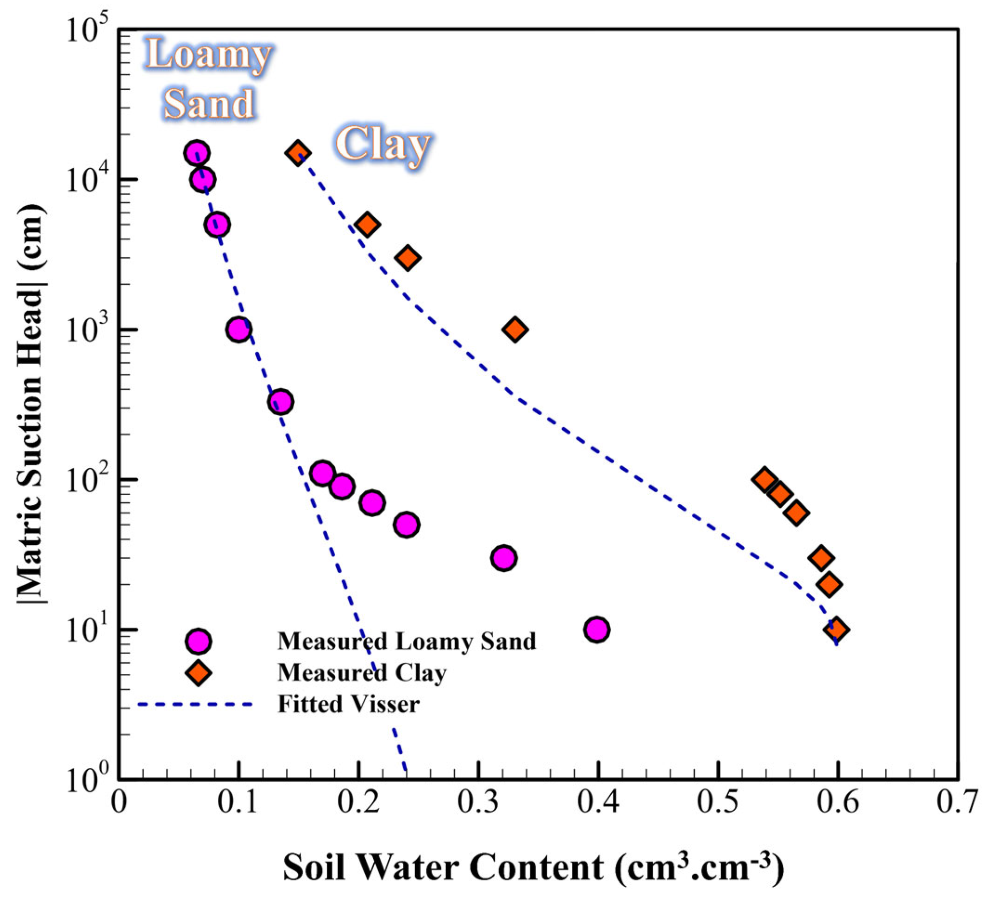
h = a φ θ b θ c
where φ is the soil porosity, and a, b, and c are model parameters. These parameters are determined for each soil by fitting the model to experimental SWRC data. Unlike conventional models, which assume abrupt changes in the SWRC at the air-entry suction, this model accounts for more gradual transitions in the lower portion of the curve. As the soil water content increases, the difference between φ and θ decreases correspondingly. When the soil water content reaches saturation (i.e., equals porosity), the value of (φ − θ) approaches zero, resulting in a matric suction of zero.
Visser [63] aimed to represent the entire SWRC using a simple mathematical function. However, as shown in Figure 2, which illustrates the SWRC for both clay and loamy sand soils, the model does not follow the typical S-shaped form of the SWRC. While the model shows good agreement with the measured SWRC at high suction values, it performs poorly at low suctions, failing to capture the gradual transition near the air-entry point.
It is important to note that when the mathematical form of the model does not align well with the shape of the SWRC, optimization methods that minimize the objective function—defined as the difference between measured and modeled suction values—tend to prioritize a better fit at higher suction values. This is because large suction values dominate the error term, causing the optimization process to favor this range to minimize the overall objective function.
Conversely, if the SWRC model were formulated such that θ is expressed as a function of h, the objective function would be defined as the difference between the measured and modeled water contents. Since changes in water content are relatively small compared to suction values, this formulation would result in a better overall fit to the experimental data across the full range of suction values. The tendency of the Visser model to fit more accurately at high suction values stems from this numerical characteristic.
In inverse methods for parameter estimation, the estimated parameters must not be strongly correlated [84]. However, as shown in Table 1, significant correlations exist between the model parameters, which negatively affect the fitting accuracy. A high correlation between parameters can lead to overestimation of one parameter and underestimation of another, resulting in non-unique parameter estimates and lower confidence in the parameter values.
Additionally, Table 2 indicates that the standard errors for parameters a and b are significantly larger than their corresponding values, particularly for loamy sand. This suggests that the calibration process is not sensitive to these parameters, which in turn increases the 95% confidence interval limits, making the model predictions less reliable.
Another limitation of the Visser model is that the term (φ − θ) can become negative when φ is estimated during the fitting process. To avoid this issue, it is advisable to either impose a constraint on φ during the fitting process or to use a measured value for φ instead of estimating it. This would help prevent unrealistic negative values and improve the model’s reliability.
An improved function to describe the SWRC was proposed by [38] in the form of Equation (6):
θ = θ r + θ s θ r 1 2   erfc   a b c + α h
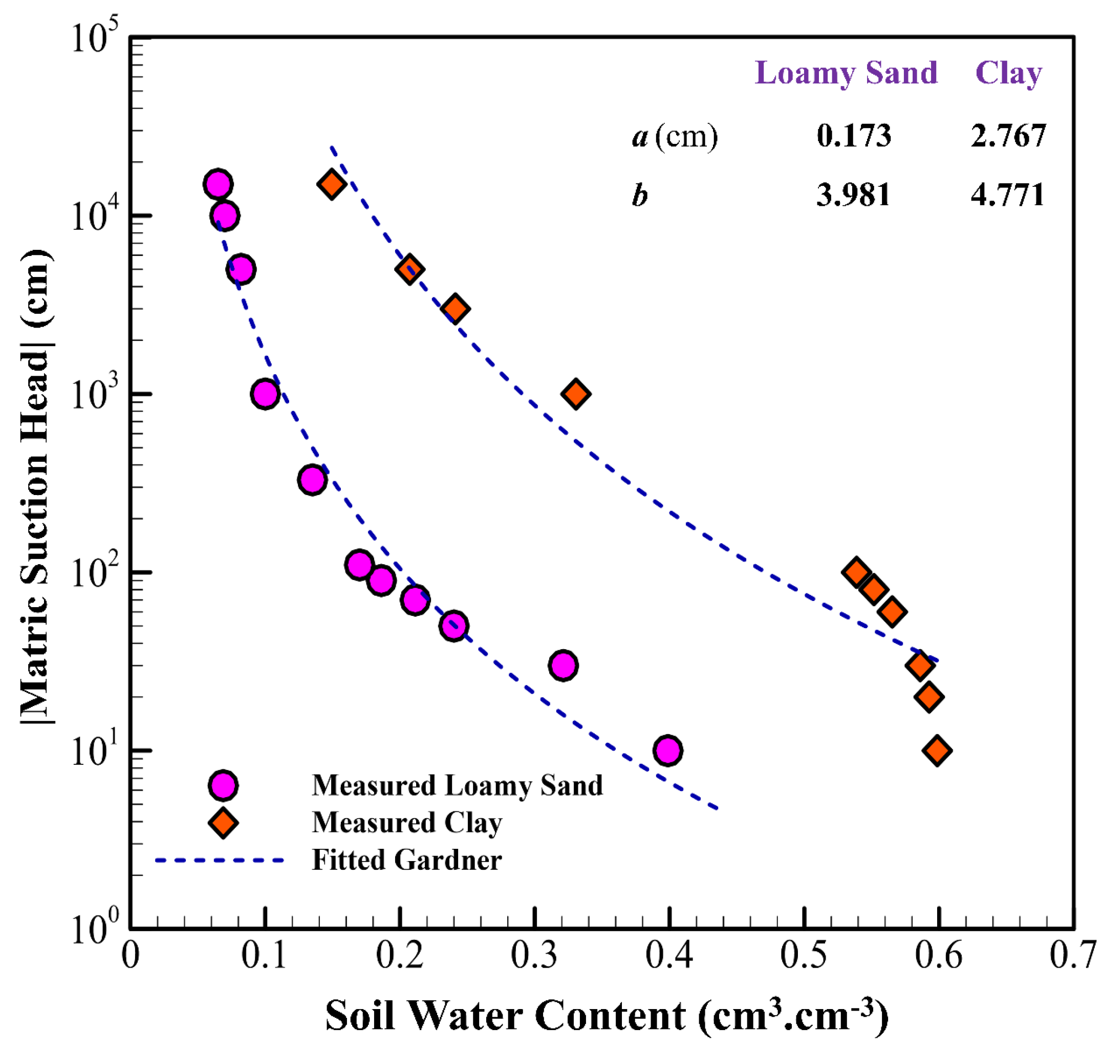
where a, b, and c are parameters defined as a function of the PSD index, α represents the inverse of the air-entry suction, and erfc is the complementary error function. It is evident that the model is sensitive to λ, which causes it to lose flexibility in describing the wet part of the SWRC. Gardner [64] argued that a significant portion of the SWRC can be represented by a power function. Approximately four years after Visser, he proposed the following simple power equation, which can be written in two forms:
θ = h a 1 b
h = a θ b
where a (L) and b are the model parameters. The mathematical structure of this model is simpler, and its parameters are easier to estimate compared to the Visser model. This model generally provides a good fit for most parts of the SWRC. However, it should be noted that it cannot adequately represent the SWRC at low suctions, as the water content approaches saturation but the matric suction does not approach zero. For suction values lower than the inflection point, the SWRC profile is parabolic. To better illustrate this, the Gardner model was fitted to two soils with fine and coarse textures. Figure 3 clearly demonstrates that the Gardner model fails to exhibit a parabolic behavior at low suctions.
By setting θr to zero in the BC model and scaling the water content parameter, Campbell [65] proposed a straightforward model as follows:
h = h a θ θ s b
θ = θ s h h a 1 b
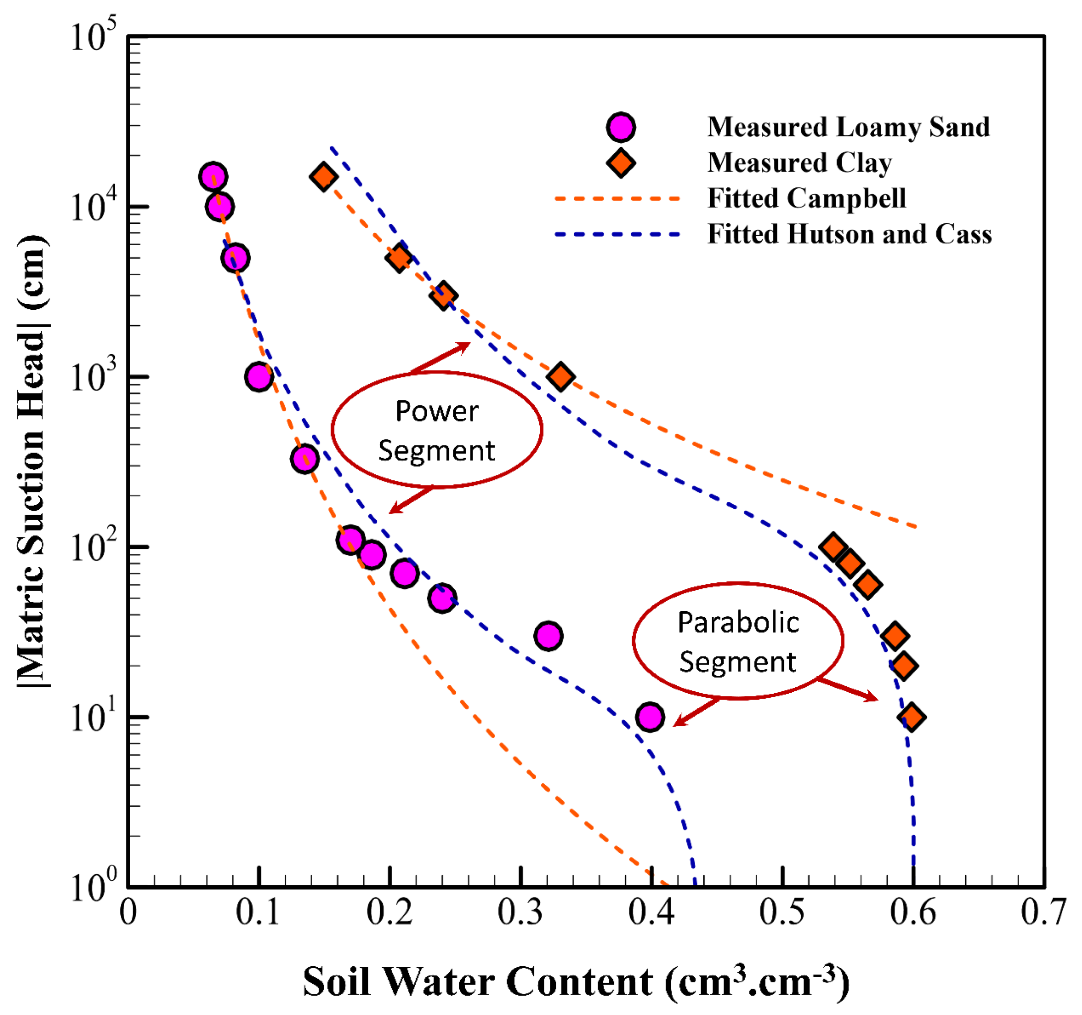
According to the Campbell model, for matric suction values less than air-entry suction, the curve predicted by the model is defective and exhibits a tail-off behavior. As soil water content increases, the matric suction decreases, but it never reaches zero. Based on Equation (9), if the soil water content reaches saturation (θ = θs), the matric suction approaches the air-entry suction (h = ha). In other words, for water content equal to saturation, the matric suction is not zero, which contradicts the fundamental nature and description of the SWRC. At saturation, the matric suction should be zero.
Like the Gardner model, the Campbell model is also incapable of representing the parabolic portion of the SWRC. Although the Campbell model incorporates the saturated water content factor, unlike the Gardner model, this addition does not result in a significant improvement. Consequently, when these two models are plotted against measured values, the resulting SWRCs overlap.
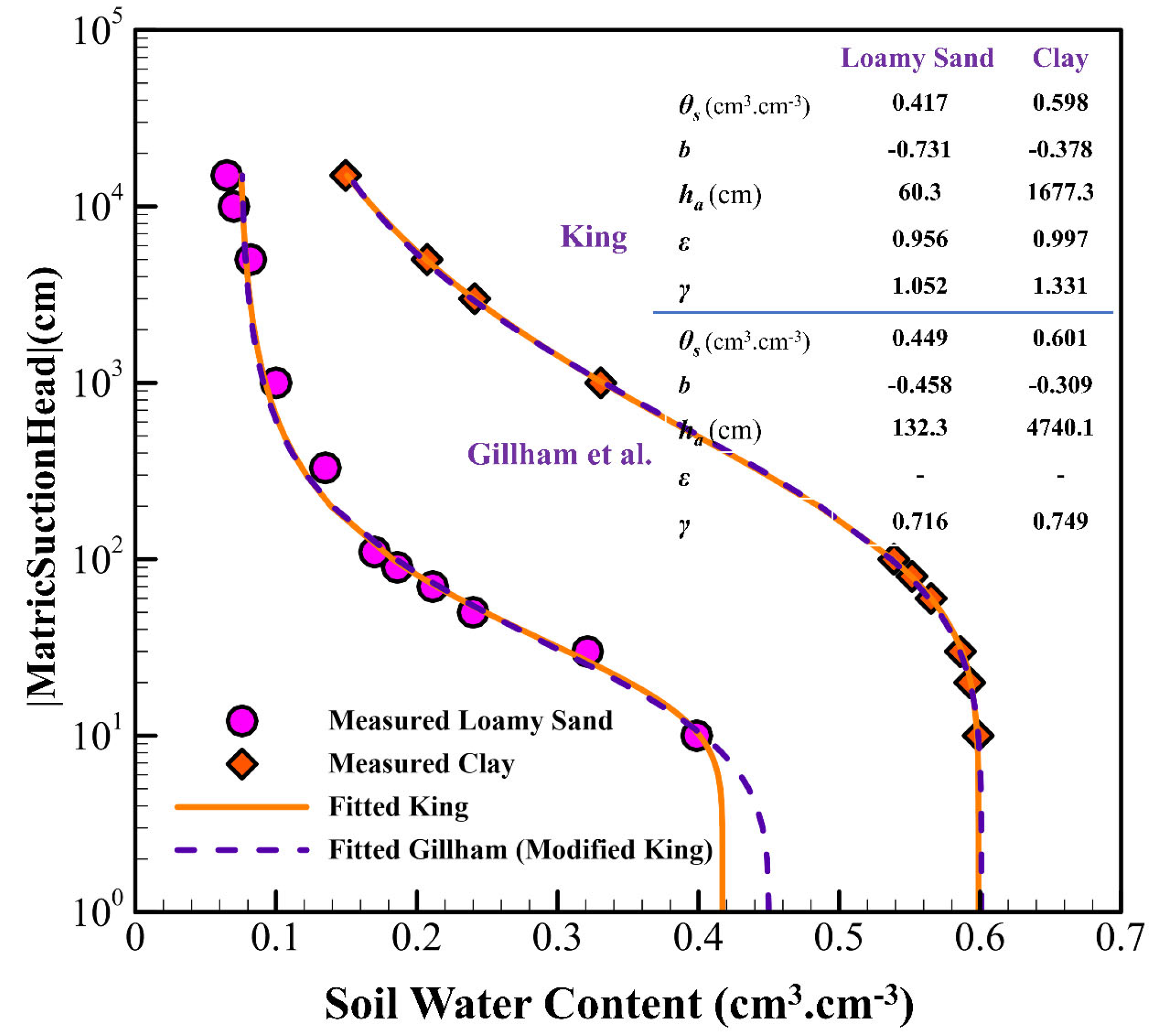
In a study conducted by Gillham et al. [66], it was shown that the King model (Equation (3)), when simplified by omitting certain parameters (notably ε), exhibited only a slight reduction in flexibility for predicting the SWRC. Figure 4 illustrates the fitting results for clay and loamy sand soils using both the King and Gillham et al. models. In the Gillham et al. (modified King) model, the ε parameter is removed, and the model is re-fitted to laboratory SWRC data using the Levenberg–Marquardt algorithm. Figure 4 clearly demonstrates how the number of adjustable parameters affects the accuracy and flexibility of the model. Despite the omission of the ε parameter, the Gillham et al. model still provides an acceptable fit.
Overall, none of the models discussed so far are able to adequately describe the parabolic curvature of the SWRC, nor can they accurately simulate the WRC curve at low suctions. In addition to these models, others were proposed by Su and Brooks [85] and Clapp and Hornberger [86]. Although these models achieved greater accuracy in simulating the SWRC compared to earlier models, they were mathematically complex, and their parameters were difficult to estimate. Consequently, they have not been widely adopted in water and soil studies.
The most practical and widely used SWRC model for simulating water and solute movement in the vadose zone is the van Genuchten [39] model (VG model). This model successfully captures the parabolic curvature of the SWRC, enabling more precise simulations of the SWRC at low suctions compared to similar models. It is expressed as follows (soil water content as a function of matric suction and vice versa):
θ = θ r + θ s θ r 1 + α h n m
h = 1 α θ θ r θ s θ r 1 m 1   1 n
where m and n are referred to as shape parameters and lack direct physical meaning, while α (L−1) represents the inverse of the air-entry suction. It is important to note that prior to van Genuchten’s work, and assuming m = 1, this equation had already been employed by other researchers [87,88,89]. The α parameter always takes values greater than zero. The amount of n is larger than one, and typically ranges from approximately 1.1 for fine-textured soils to values exceeding 4 for coarse-textured soils.
Some researchers, such as Leij et al. [31], have suggested that n can be expressed in terms of λ from the Brooks and Corey model, where n = λ + 1. The m parameter, on the other hand, varies between zero and one. These shape parameters allow the van Genuchten model to describe a wide variety of soil water retention behaviors, making it highly versatile for different soil types.
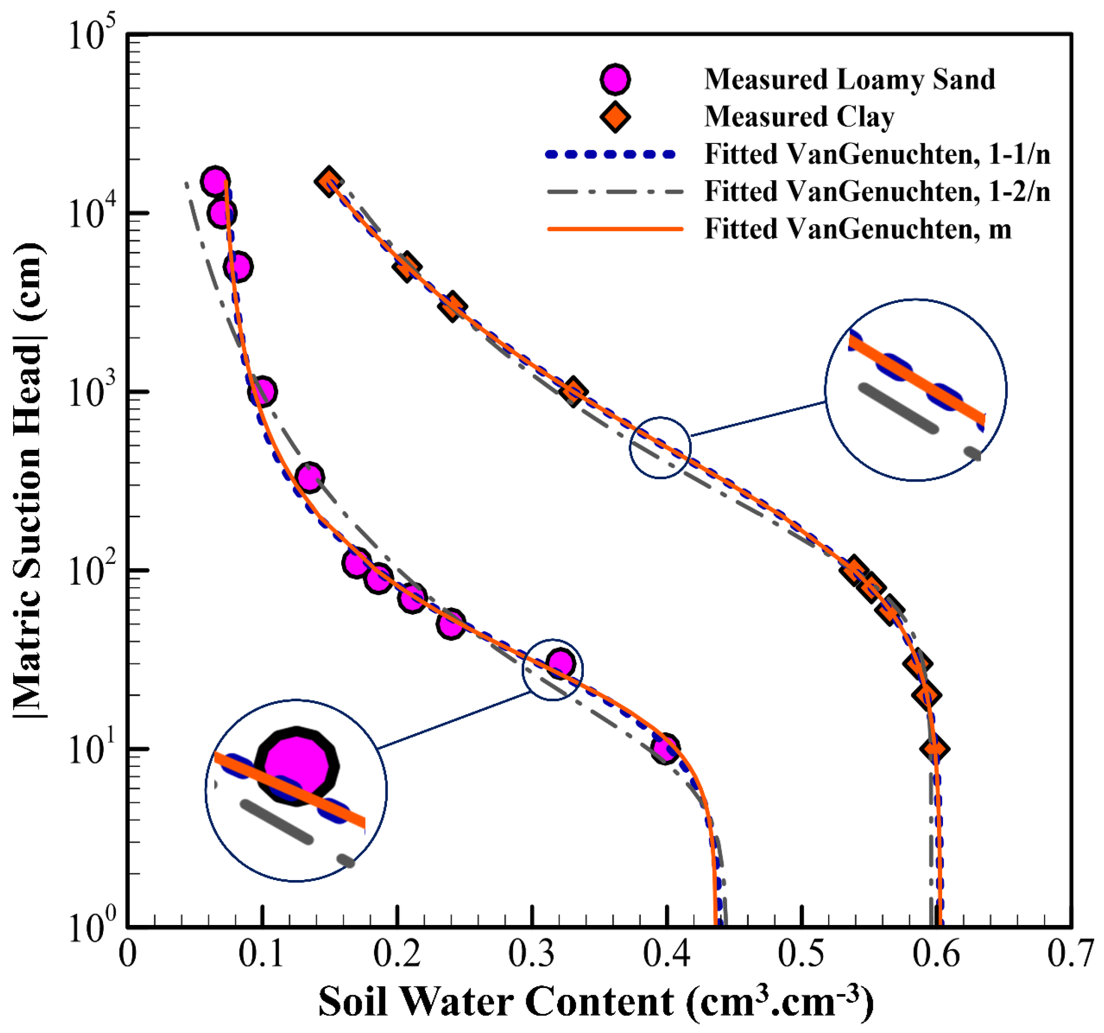
According to Equation (12), the VG model near saturation accounts for the physical properties influencing the SWRC but has an inherent weakness at the residual water content. When the soil water content equals saturation, the matric suction is zero. However, for water content equal to or below θr, the model diverges. van Genuchten observed the best fit between the model and the measured SWRC values when involving m as the exponential variable. For most soil types, replacing m with 1 − 1/n or 1 − 2/n achieves good consistency between the model output and experimental data. Applying these constraints reduces the number of estimated parameters, simplifying the equation and decreasing the correlation between parameters.
When fewer parameters are estimated, the correlation between parameters during model fitting decreases. Specifically, m and n are inherently highly correlated. By replacing m with 1 − 1/n, m is effectively eliminated, thereby removing its correlation with other parameters. On the other hand, keeping m as a variable can increase parameter correlation, potentially leading to non-unique estimated parameters. In particular, high correlation between m, n, and α can result in over- or underestimation of these parameters.
To illustrate this, the correlation matrix of the parameters for two scenarios—one including m as a variable and the other replacing it with 1 − 1/n—is presented in Table 3. When m is included as a variable, its correlation with n and α increases significantly. High parameter correlation means that the value of one parameter affects the other, which may lead to overestimation of one and underestimation of the other. Consequently, the uniqueness of the estimated parameters cannot be guaranteed.
To evaluate the VG model’s fit to experimental data, the model was applied to experimental values for clay and loamy sand textures under three conditions for m: m as a variable, m = 1 − 1/n, and m = 1 − 2/n. According to Figure 5, for the first two conditions, there is no significant difference in the SWRC fit. Therefore, 1 − 1/n is often used instead as a replacement for m. In general, using m as a variable provides the best fitting results for many soil textures.
As demonstrated, the Brooks and Corey, Gardner, and Campbell models are not fully capable of fitting the measured SWRC, particularly in the low-suction range. These models fail to produce the S-shaped curvature and cannot represent the downstream parabolic curvature. In contrast, VG-type models, due to their sigmoid behavior, generate an S-shaped curve and fully capture the parabolic curvature of the SWRC.
Although the VG model does not explicitly consider the matric suction at the air-entry suction and its parameter correlation makes it sensitive for some soils, its key advantage lies in having an inflection point. This feature enables excellent fitting to measured data, particularly at high water content values.
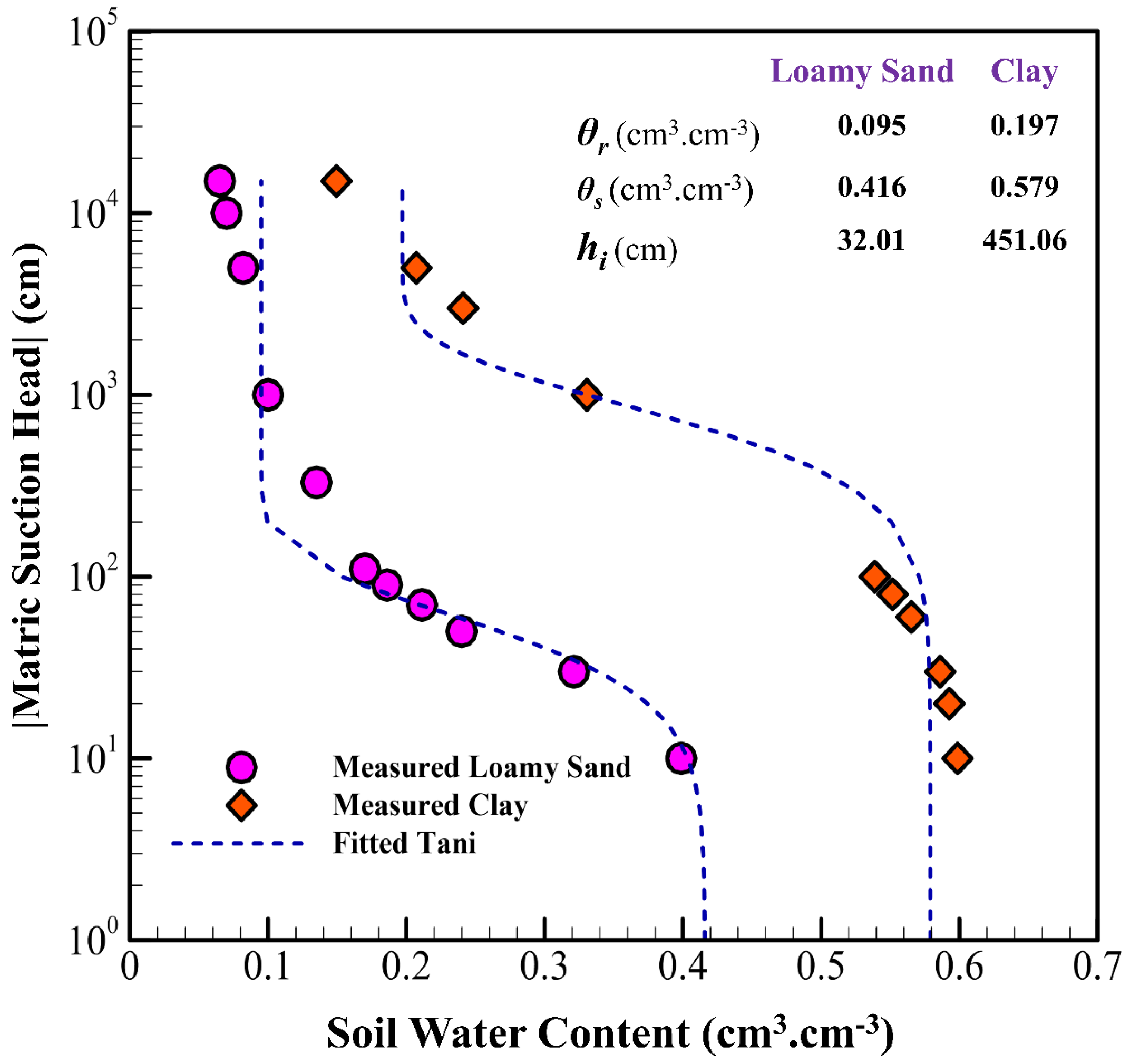
One of the essential criteria for SWRC models is their ability to conform to the inflection point. Tani [67] investigated an exponential model that explicitly considers the matric suction at the inflection point of the SWRC:
θ = θ r + θ s θ r 1 + h h i exp h h i
where hi (L) represents the matric suction at the inflection point of the SWRC. The Tani model is simpler compared to the VG and BC models, featuring fewer parameters. This simplicity results in relatively low parameter correlation, making the model more reliable. Despite its simplicity, for matric suction values below the inflection point suction, the model satisfies the parabolic curvature constraint of the SWRC and successfully predicts the general S-shape of the curve.
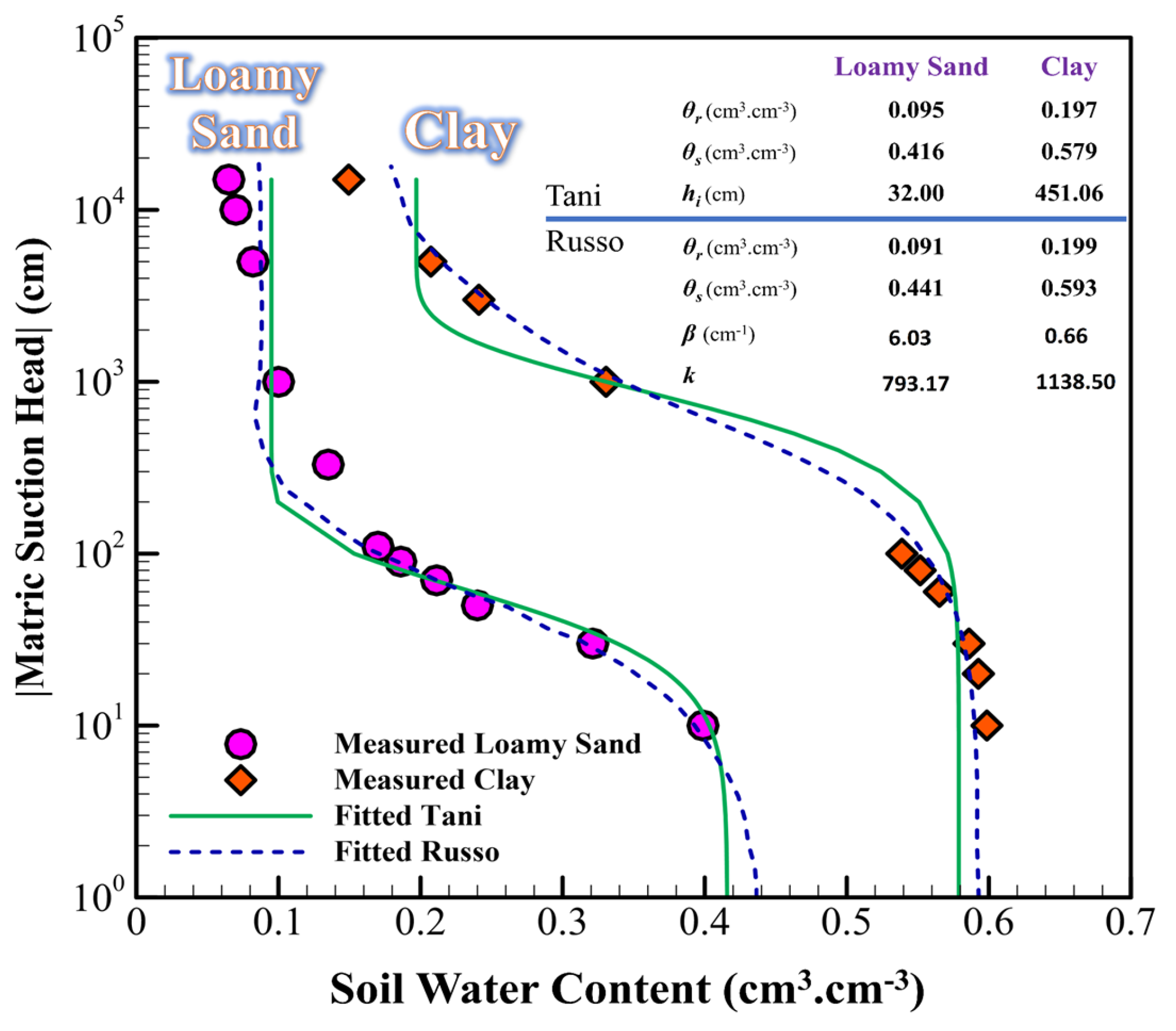
However, a key disadvantage of the Tani model is its inability to fully fit the measured SWRC, particularly at high suction values. Figure 6 illustrates how this model predicts the SWRC for fine-textured and coarse-textured soils. While the model demonstrates reasonable agreement with experimental data in the low-suction range, its accuracy diminishes as suction values increase, limiting its effectiveness in capturing the full behavior of the SWRC across the entire range.
Despite this limitation, the simplicity and low correlation between parameters make the Tani model a practical option for certain applications, especially when computational efficiency or limited data availability is a priority.
As previously mentioned (Equations (11) and (12)), the VG model originally includes five adjustable parameters. Due to the high correlation between the parameters m and n, van Genuchten addressed this issue by employing m = 1 − 1/n, aiming to mitigate the effect of parameter correlation. About five years later, van Genuchten and Nielsen [90] proposed that m and n could be treated as completely independent parameters. However, they concluded that this approach yielded better results only for a limited range of SWRC data, typically in the wet range. Including both m and n as independent parameters in the model introduces problems of uniqueness in parameter estimation, reducing precision in the dry range and leading to a lack of physical meaning in the estimated parameters [91].
McKee and Bumb [68] proposed an exponential model, known as the Boltzmann model, which consists of only two parameters for estimating the SWRC. Due to the correlation and interaction between these parameters, their individual effects on the SWRC are difficult to discern. This model is a simplified version of the Tani model and is expressed as follows:
θ = θ r + θ s θ r   exp h h i
h = h i   ln θ θ r θ s θ r
Hutson and Cass [40] developed their model based on the earlier research by Campbell [65]. A critical flaw in the Campbell model is its inability to accurately estimate the measured SWRC for suctions below the air-entry value. To address this limitation, Hutson and Cass [40] proposed a piecewise-modified SWRC function that combines exponential and parabolic components. This hybrid approach improves the model’s flexibility and accuracy across the suction range. The proposed hybrid function is expressed through Equations (16)–(19), which describe its formulation in detail.
θ = θ s h a 1 b θ < θ i
θ = θ s θ s h 2 1 θ i θ s a 2 θ i θ s 2 b θ θ i
h = a θ θ s b h > h i
h = a 1 θ θ s 0.5 θ i θ s b 1 θ i θ s 0.5 0 h h i
In the above equations, a and b are empirical parameters. The parameter a has the dimension of length (L) and serves as a correction factor, replacing the air-entry suction (ho) in the model. The parameter b is dimensionless and represents the slope of the SWRC. Additionally, the parameters hi and θi can be determined using the following equations:
h i = a 2 b 1 + 2 b b
θ i = 2 b θ s 1 + 2 b
To highlight the parabolic feature of the Hutson and Cass model and compare it with the Campbell model, both models were fitted to fine- and coarse-textured soils (Figure 7). The results demonstrate that the Hutson and Cass model effectively resolves the inherent limitations of the Campbell model, particularly in adapting to the SWRC at low suctions. This model eliminates the SWRC discontinuity observed in the Campbell model and ensures that, at water content equal to saturation, the matric suction approaches zero.
Russo [69] introduced a significant amendment to the Tani [67] model by incorporating an additional parameter, thereby improving its flexibility and adaptability. The modified Russo model is expressed as follows:
θ = θ r + θ s θ r 1 + β h exp β h 2 / k + 2
where β is an empirical parameter added to the equation as a substitute for the inflection point. The parameter k, introduced by Mualem [92], is also included in the model. These parameters can be estimated by fitting the modified model to observed SWRC data. The adjustments made to the Tani model improved the accuracy of the modified Russo model in capturing the measured SWRC, particularly at low suction values. However, for high suction values, the model still exhibits limitations in approximating the laboratory-measured SWRC.
Figure 8 illustrates the quality of fitting for both the Tani and Russo models, highlighting the improvements introduced by Russo while also showing the areas where the model’s performance remains suboptimal.
It is worth noting that the correlation matrix of the Russo model indicates low correlation between parameters, meaning they do not significantly affect each other. However, the standard error associated with the parameter k is relatively large (Table 4). As a result, the 95% confidence limits for this parameter are broad, leading to reduce reliability and lower confidence in its estimated value.
Vogel and Cislerova [41] argued that, although the VG model successfully approximates the parabolic portion of the SWRC, it lacks sufficient adaptability for very low suctions (near saturation). To address this limitation and enhance the model’s flexibility in this range, they proposed a modification to the VG model, represented in the form of Equations (23) and (24):
θ = θ r + θ m θ r 1 + α h n m
h = 1 α θ θ r θ m θ r 1 m 1   1 n
It is notable that Vogel and Cislerova replaced θs with θm, an auxiliary fitting parameter with no physical meaning. In their corrected model, θm is determined such that the absolute value of h(θs) approaches 2 cm. This modified model is particularly recommended for fine-textured soils, with a narrow range for n (1 < n < 1.3).
Accurate descriptions of water storage and movement in the vadose zone rely heavily on precise predictions of the SWRC and hydraulic conductivity (HC) functions. Most hydraulic functions perform effectively within the range of residual to saturated water content (θr < θ < θs). However, they are generally more accurate in the wet region of the SWRC and struggle in the dry and very dry regions, especially beyond the wilting point. Furthermore, conventional SWRC models exhibit a fundamental weakness in simulating water vapor movement.
A review of the literature shows that interest in modeling the SWRC in the oven-dry region began in the 1990s. The matric suction value for the oven-dry region can be estimated by fitting SWRC models to observed data. Although modeling the SWRC across the full water content range (0 < θ < θs) increases model flexibility and improves its fit to measured values, it introduces challenges. Specifically, the correlation between oven-dry matric suction and other parameters, as well as the uniqueness problem, leads most researchers to use a fixed value for oven-dry suction.
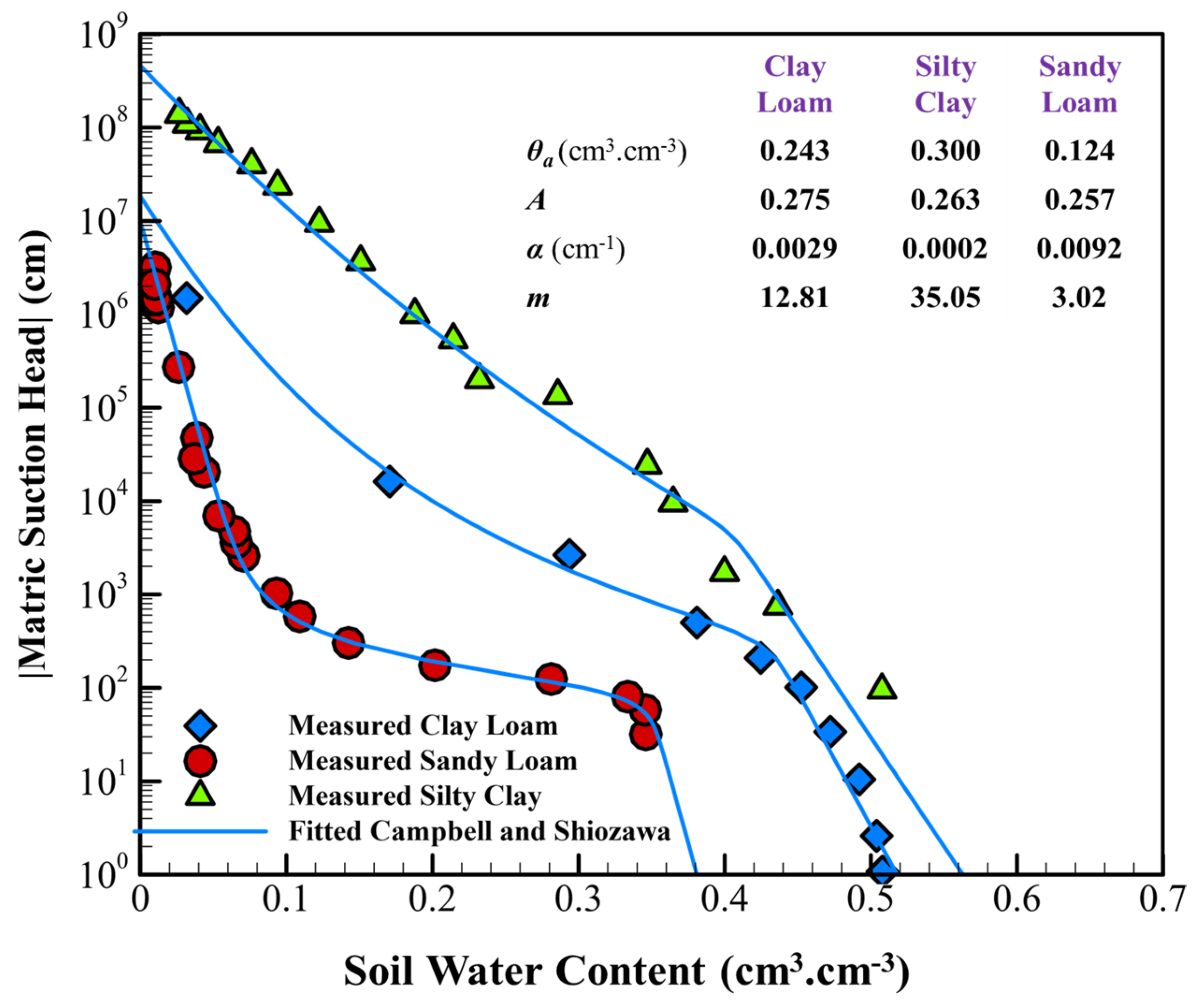
Despite these challenges, some researchers have developed models to predict matric suction across the entire water content range, from saturation to oven-dry conditions. For instance, Campbell and Shiozawa [42] (CS model) proposed a reformulated equation based on a VG-type model. In their approach, the adsorptive water term is incorporated in place of the residual water content, as follows:
θ = θ a 1 ln h ln h O + A 1 1 + α h 4 1 m
where the first term on the right-hand side refers to the adsorptive water, and m, A, and θa are curve-fitting parameters. The parameter ho is defined as the matric suction at the oven-dry conditions. The inclusion of the adsorptive water term allows the CS model to extend its applicability to the very dry region of the SWRC, offering a more comprehensive description of water retention across the full range of water contents.
This model addresses the limitations of conventional SWRC models by accounting for adsorptive water, which dominates in the oven-dry region. However, determining the parameter ho and fitting the model to experimental data can be challenging due to the increased complexity and potential parameter correlations. Figure 9 illustrates how the CS model adapts to both the wet and dry regions of the SWRC for fine- and coarse-textured soils, demonstrating its versatility compared to traditional models. Particularly, Figure 9 illustrates the fit of the CS model to three soil types (with matric suction data measured from saturation to oven-dry conditions) of varying textures, along with the estimated parameter values. It is worth noting that, to reduce the correlation between model parameters, ho was fixed at 106 kPa (≈107 cm-H2O), which helped decrease the model’s sensitivity to parameter multiplicity.
One of the main limitations of the CS model is its inability to estimate the water content for matric suction equal to zero (h = 0). As shown in Equation (25), the model becomes undefined under these conditions. Additionally, a noteworthy drawback is the high correlation between parameters for certain soils, which may reduce the reliability of the parameter estimates.
In 1994, Mehta et al. [43] introduced a new model (MSN) as an improvement over the CS model [42]. This new model combined elements of the VG and CS models, aiming to enhance flexibility and accuracy. The MSN model is expressed as follows:
θ = a 1 + α h n m + b 1 ln h + 1 c
where a, b, and c are the fitting model parameters. Unlike the previous model [43], which is undefined at zero matric suction, the MSN model is capable of predicting θs values when h = 0. However, due to the large number of parameters involved (six in total: a, b, c, α, n, and m), there is a very high correlation between the model parameters, which can complicate their estimation and reduce the reliability of the model.
Most of the models presented in the literature during the 1990s focused on the oven-dry region of the SWRC. By modifying traditional models, researchers aimed to generalize them to cover the entire range of the SWRC. For instance, Rossi and Nimmo [44] proposed that, in the oven-dry region of the SWRC, soil water content can be approximated as a logarithmic function of the matric suction with reasonable accuracy.
This two-segment model combines the BC model for a liquid phase and a logarithmic function for the adsorption region. At a specific point, referred to as the junction (or matching) point, the model transitions from the BC equation to the logarithmic function. By incorporating this concept into the BC model, they developed a new modified model expressed as follows:
θ = θ s 1 α h h e 2 0 h h j
θ = θ s h e h λ h e h o λ + β ln h o h h j h h o
where α is an index that affects the parabolic portion of Equation (27), β represents the slope of the tangent line at the junction point, hj denotes the matric suction at the junction point (where the two connected segments meet), and he and ho refer to the air-entry and oven-dry matric suctions, respectively.
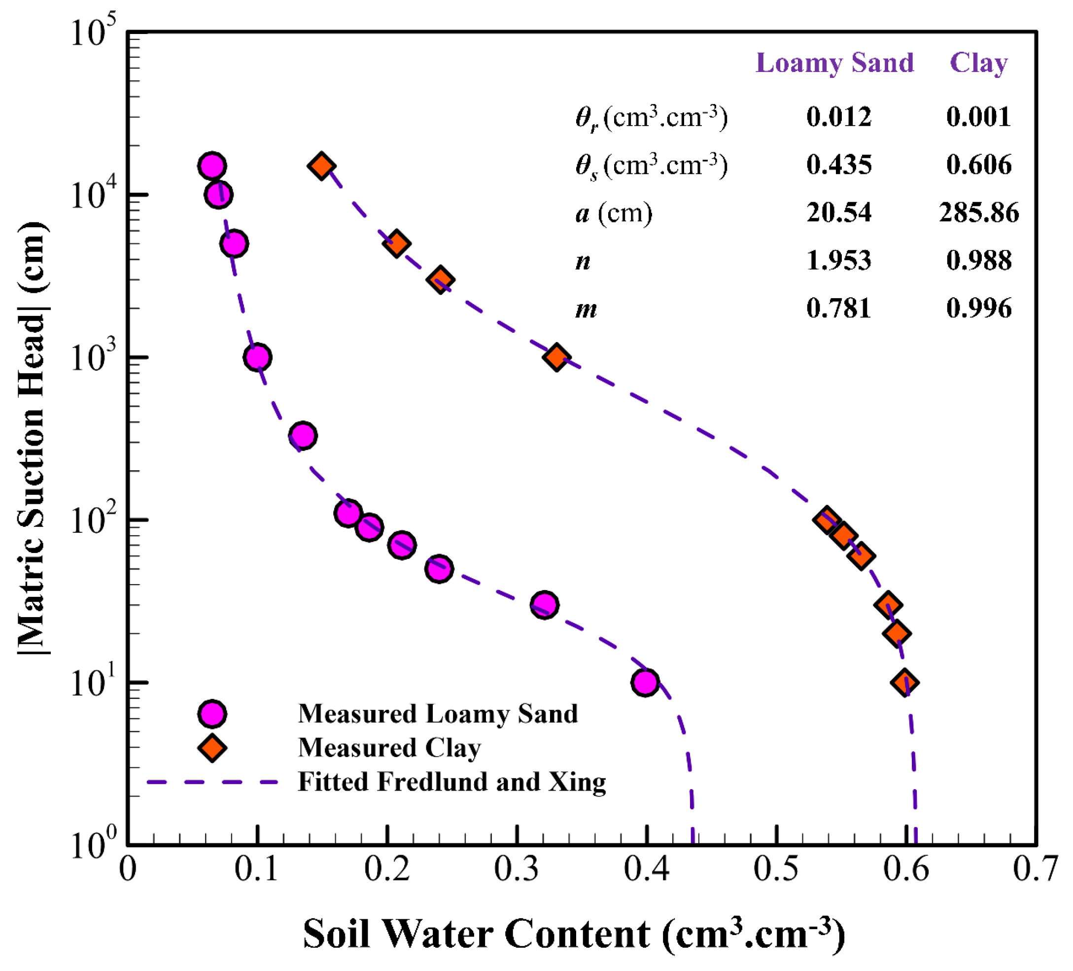
Fredlund and Xing [45] (FX model), based on the concept that the SWRC is a function of PSD, developed a five-parameter model designed to capture the entire shape of the retention curve:
θ = 1 ln 1 + h h r ln 1 + 10 6 h r θ s ln e + h a n m
where a, n, and m are empirical shape parameters, and hr represents the estimated matric suction associated with the residual water content. In Figure 10, the fitting results of the FX model to fine- and coarse-textured soils are shown, along with the corresponding values of the estimated parameters.
Taking into account bimodal PSD, Zhang and van Genuchten [70] proposed a new closed-form expression to predict the SWRC, aiming to improve its accuracy for soils with complex structures:
θ = θ r + θ s θ r 1 + C 1 δ h 1 + δ h + C 2 δ h 2
where δ is referred to as the scaling factor, and C1 and C2 are empirical parameters that define the shape of the SWRC. Kosugi [46], at the beginning of his extensive investigations, initially proposed a parametric lognormal model with three adjustable parameters. By 1999, he refined the model to make it simpler and more user-friendly.
In 1996, to further simplify the model and reduce the correlation between its parameters, Kosugi suggested that by setting the least significant parameter to zero, the model could still achieve an acceptable fit to laboratory SWRC data. This approach transformed the original three-parameter lognormal model into a more streamlined two-parameter version. The Kosugi [46] model is expressed as follows:
θ = θ = θ r + 1 2 θ s θ r erfc ln h a h h a h o n 2 2 n h > h a θ s h h a
where n, ha, and ho are the model parameters with physical meaning. These parameters are directly related to the logarithmic mean and standard deviation of the PSD for any soil sample. Specifically, ha represents the air-entry suction, n corresponds to the standard deviation of the transformed pore capillary pressure distribution (related to the width of the pore radius distribution), and ho denotes the capillary pressure at the inflection point. The remaining parameters have been already defined.
In 1996, to simplify the model (Equation (31)) and reduce the number of parameters, Kosugi proposed setting ha to zero. He demonstrated that this adjustment allowed the model to retain an acceptable fit to the SWRC while reducing its complexity.
θ = θ r + 1 2 θ s θ r erfc ln h h o n 2 2 n
This model produces acceptable fits for SWRCs that lack a distinct air-entry pressure.
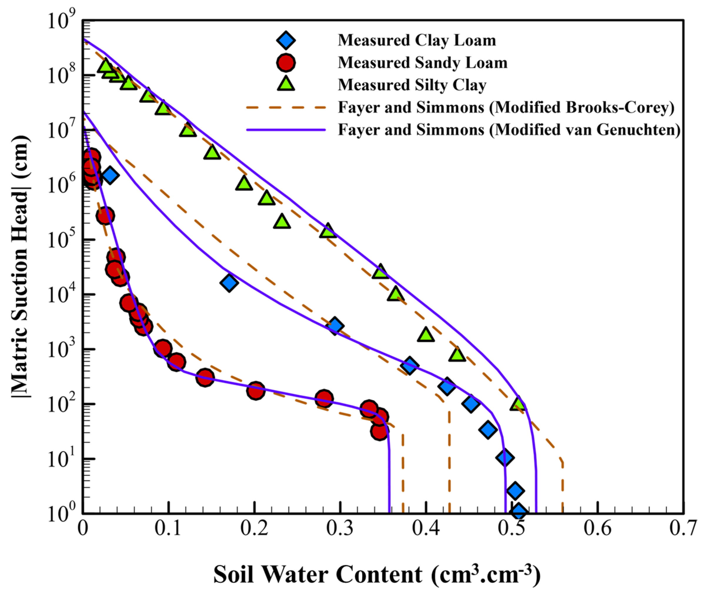
As previously mentioned, the BC and VG models are unable to calculate matric suction for water contents less than or equal to the residual value. In an effort to address this limitation and create a model capable of covering the entire SWRC from saturation to oven-dry conditions, Fayer and Simmons [47] proposed a solution. By incorporating the equation for adsorptive water content suggested by Campbell and Shiozawa [42], they modified the BC and VG models. The resulting models, FSVG and FSBC, are expressed by Equations (33) and (34), respectively.
θ = θ a 1 ln h ln h 0 + θ s θ a 1 ln h ln h 0 1 + α h n m
θ = θ a 1 ln h ln h 0 + θ s θ a 1 ln h ln h 0 α h λ α h 1 θ s α h < 1
Indeed, in the above two equations, the residual water content parameter in the BC and VG models is replaced with the adsorptive water content equation. The fitting performances of the modified VG (FSVG) and BC (FSBC) models to the measured SWRC, spanning from saturation to oven-dry conditions for three different soil textures, are shown in Figure 11.
It is important to note that the modifications applied to the BC and VG models primarily extend their water content domain, but they do not alter the general trend of the matric suction curve. Consequently, the modified BC model retains its inherent limitation for matric suctions below the air-entry value. Additionally, as indicated by Equations (33) and (34), these models are undefined at zero matric suction (h = 0), and the water content does not equal the saturation (θs). Due to the number of parameters and the potential correlation between them, the FSVG and FSBC models may face issues of parameter uniqueness.
Assouline et al. [49] proposed their SWRC model based on the following two hypotheses:
  • Soil particle size distribution, which directly influences soil structure, is a result of a process of uniform random fragmentation.
  • The conversion of solid particle volume to pore volume follows a power function, with the equation constant being proportional to the particle shape produced by fragmentation.
Based on their conceptual framework, they introduced Equations (35) and (36):
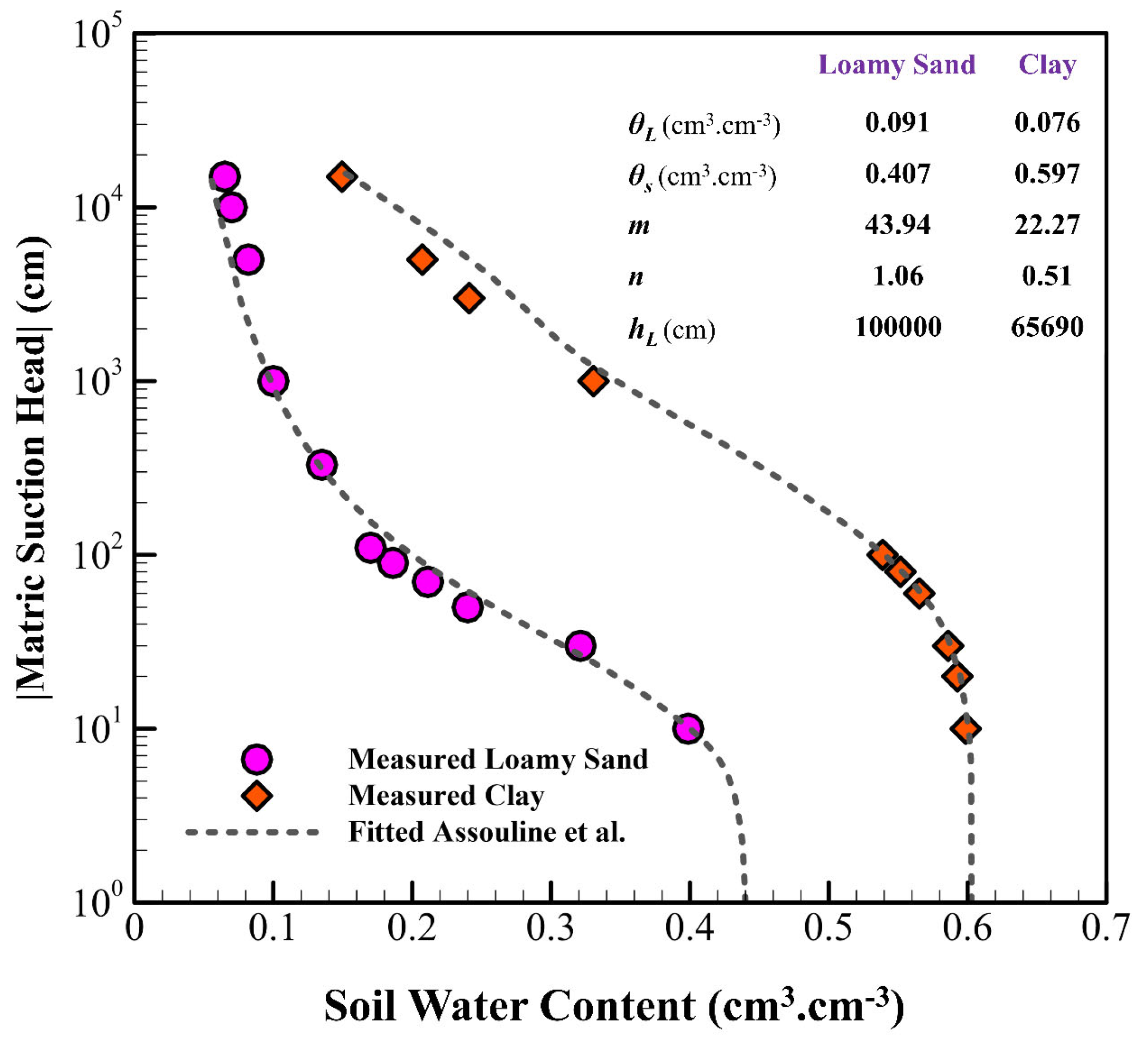
θ = θ L + θ s θ L 1 exp m h 1 h L 1 n
h = h L 1 + 1 m   ln 1 θ θ L θ s θ L 1 n 1
where θL refers to the water content at which the hydraulic conductivity becomes negligible, and hL, represents the matric suction corresponding to this very low water content. This developed model is undefined for h = 0. The parameters m and n are curve-fitting parameters that are influenced by particle shapes, packing configuration, and PSD.
In Figure 12, the fitting results of the Assouline et al. [49] model for fine- and coarse-textured soils are plotted, along with the values of the estimated parameters.
Webb [50] proposed a two-segment model that covers the entire range of the SWRC, from saturation to oven-dry conditions. This two-phase SWRC model incorporates the VG model for the liquid phase and a linear function for the adsorption region. Similarly to the Rossi and Nimmo [44] model, the transition between the VG equation and the linear equation occurs at a junction (or matching) point.
The linear relationship between θ and h for the dry region, represented in the format of a semi-log plot, is described by Equations (37) and (38):
θ = k log 10 h log 10 h m + θ m
h = 10 θ θ m k +   log 10 h m
where k represents the slope of the tangent line at the junction point and is identical to d θ VG h m / log 10 h . The parameters θm and hm correspond to the water content and matric suction at the matching point, respectively.
Groenevelt and Grant [51] introduced the following model for the SWRC:
θ = θ a + k 1 exp k 0 h a n exp k 0 h n
h = k 0 ln exp k 0 h a n θ θ a k 1 1 n
where k1, k0 and n are curve-fitting parameters adjusted from experimental data. In this model, θa represents the water content corresponding to the capillary suction ha. Groenevelt and Grant identified a as a point where matric suction is extremely high and soil water content is very small. To avoid disagreements regarding the definition of residual water content, they specified that θa is the water content at the wilting point and substituted ha with 15,000 cm-H2O in Equations (39) and (40).
It should be noted that incorporating the wilting point introduces some limitations into the model. This point may not be present in the collection of measured points for the empirical SWRC, or if measured, fitting errors at this point are highly likely.
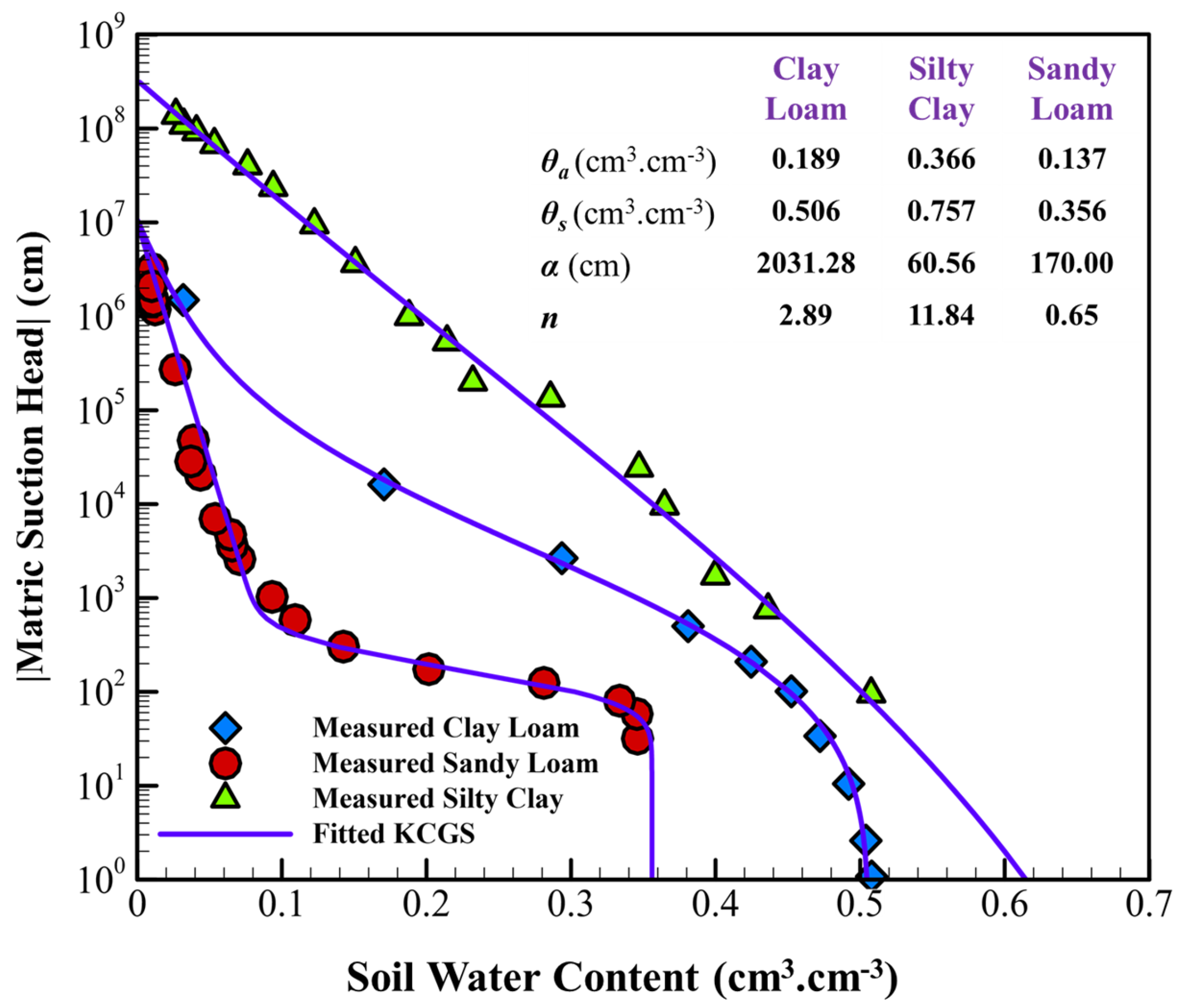
Khlosi et al. [52] (KCGS model) combined the concept of soil adsorptive water from Campbell and Shiozawa [42] with a revised version of the Kosugi [93] model to comprehensively describe the corresponding matric suction of water content across the entire range of conditions, from saturation to oven-dry, as follows:
θ = θ a 1 ln h ln h o + 1 2 θ s θ a 1 ln h ln h o erfc   ln h α 2 n
where the five model parameters are θa, θs, ho, α, and n. The parameters θa and ho have similar definitions as in the Fayer and Simmons [47] models, while the remaining parameters are defined as in the Kosugi model. Once again, erfc refers to the complementary error function.
The primary advantage of the KCGS model over the Kosugi model is its ability to describe matric suction across the entire range of the SWRC, from saturation to oven-dry conditions. The fitting results of the KCGS model to the measured SWRCs are plotted in Figure 13.
Khlosi et al. [52] claimed that a notable strength of their model is its capacity to estimate the full SWRC range even when calibrated using a limited dataset, including only water content measurements at matric suctions greater than −100 kPa.
As explained in the VG model, the inability to estimate matric suction at the air-entry suction (ha) is often cited as a weakness. To address this limitation, Ippisch et al. [53] reformulated the original VG model, incorporating ha and proposing a two-segment model to better predict the SWRC:
θ = θ r + θ s θ r 1 + α h n 1 + α h a n m h > h a θ = θ s h h a
h = 1 α 1 + α h a n θ θ r θ s θ r 1 m 1 1 n θ   < θ s h = 0 θ = θ s
All parameters in Equations (42) and (43) have been previously defined.
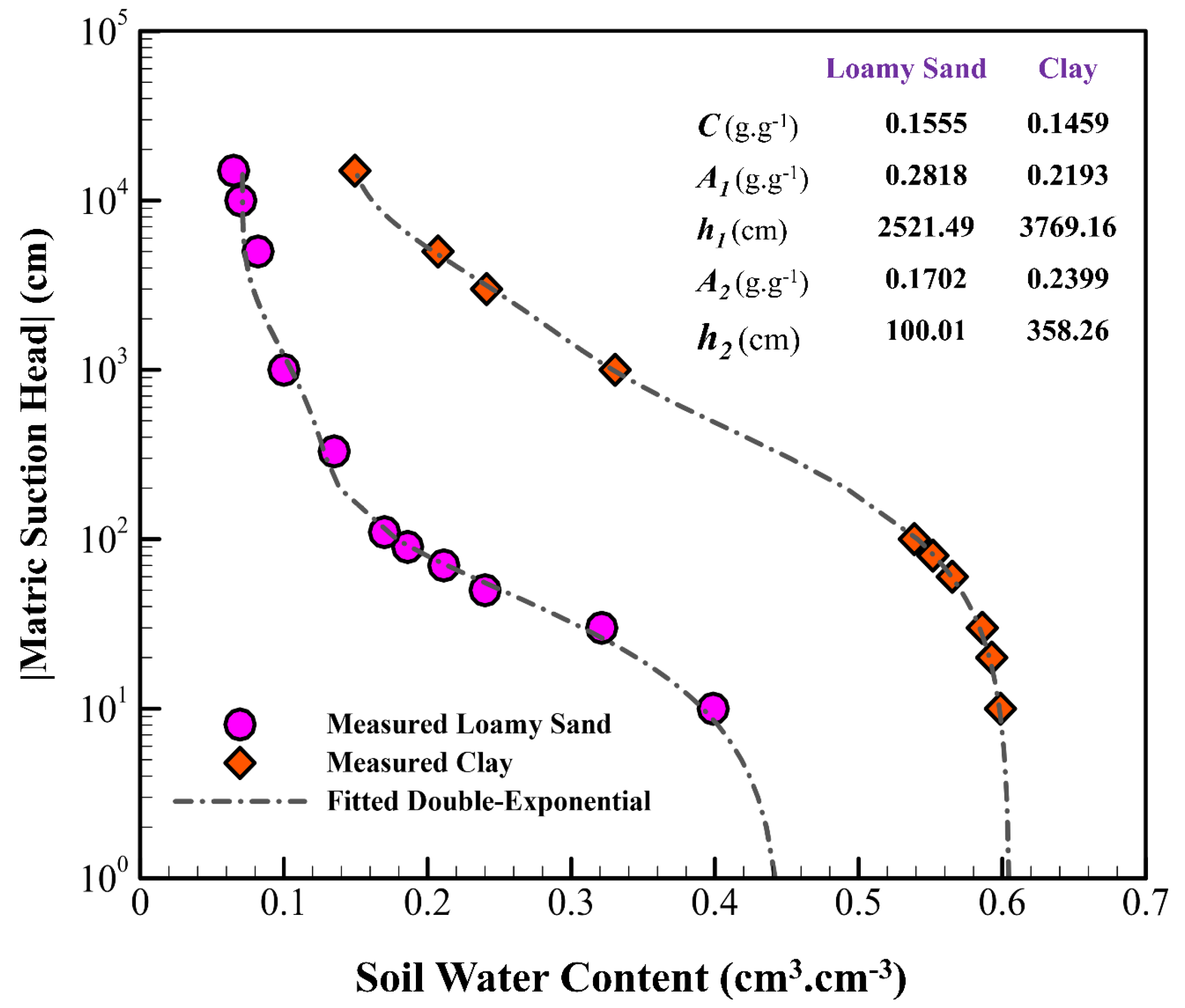
Dexter et al. [54] proposed a double-exponential model including five adjustable parameters of physical significance. The parameters in this model correspond to the soil matrix and the structural pore space. In essence, the pore configuration within the soil determines the shape of the function. The proposed double-exponential function is expressed in the form of Equation (44):
w = C + A 1 e h h 1 + A 2 e h h 2
where w is the gravimetric soil water content (M·M−1) associated with the matric suction (L), and C represents the asymptote of the model, which corresponds to the gravimetric residual water content (M·M−1) in the soil (i.e., the soil water as the matric suction approaches infinity). A1 and A2 are model parameters related to the PSD and the soil structure, respectively. h1 and h2 correspond to the matric suction levels at which water drains from the textural (matrix) and structural pore spaces, respectively.
It can be inferred that the Dexter model is bimodal. The first part of the model represents the matrix pores, while the second part accounts for the effects of the structural pore spaces on the SWRC. Experience has shown that one limitation of this approach lies in the mathematical similarity of the terms. Specifically, during model fitting to the measured SWRC, if the initial conditions for parameter estimation are not properly defined, the roles of the first and second terms may switch.
Despite this limitation, the double exponential model proves to be more accurate than the VG model and better fits the measured SWRC. Additionally, the internal correlation among parameters in this model is lower than in the VG model. However, unlike the VG model, which produces a single unique inflection point, the double exponential model does not have a single distinct inflection point. Figure 14 illustrates the fitting of this model to fine- and coarse-textured soils.
Omuto [55] introduced another bi-exponential model, conceptually very similar to the Dexter model, which is expressed by Equation (45):
θ = θ r + θ 1 e α 1 h + θ 2 e α 2 h                             h < 0 θ s                                                                                                                 h = 0
Omuto, in his study, considered segregated residual and saturated water contents in the format of (θr1, θs1) and (θr2, θs2) for the structural and textural pore spaces, respectively. He also defined α1 and α2 as the inverse of the air-entry potential for the structural and textural pore spaces, respectively.
Grant et al. [56] aimed to achieve a more precise estimation of θa, previously introduced in the study by Groenevelt and Grant [51]. To improve the model’s flexibility and performance, θa was defined as the anchor point. Based on the available dataset, three modes for θa were considered: the oven-dry point (θa = 0), the saturation coordinate (θa = θs), and the wilting point (θa = θwp). The corresponding values of ha for these three conditions were assumed to be 104.9, 0, and 15,000 cm-H2O, respectively.
Romano et al. [57], similarly to Dexter et al. [54], classified soil pores into two categories based on textural and structural water retention behaviors. Although it is practically impossible to physically distinguish structural pore spaces from textural (matrix) pores, this classification can be useful conceptually. Structural pores, located between soil aggregates, retain water at low matric suction, while the smaller textural (matrix) pores retain water at higher matric suctions.
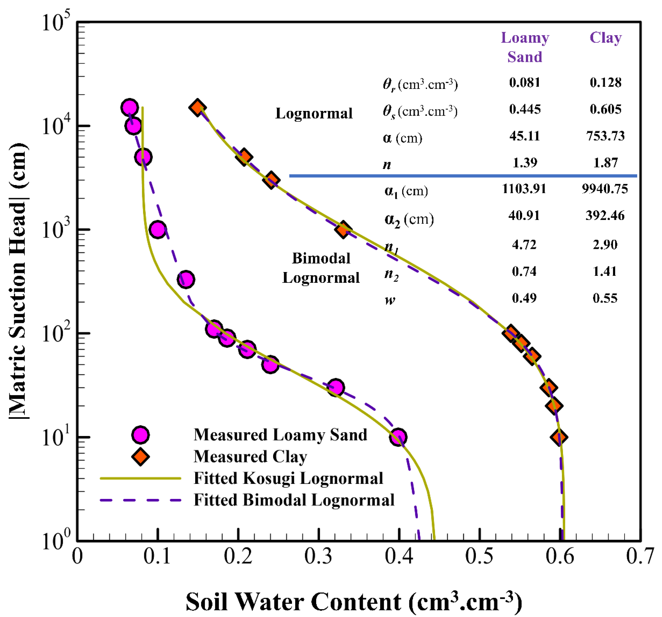
Romano utilized the two-parameter lognormal model from Kosugi [48] as the unimodal function. In this context, the slope changes of the SWRC exhibit two maximum values, which correspond to the structural and textural pore spaces. The two-parameter lognormal model was assigned to represent the textural component of the soil, while an additional component was introduced to account for the structural pores. This approach led to the development of a bimodal lognormal function for estimating the SWRC.
In essence, the bimodal lognormal function is defined by the linear superposition of two distinct pore domains: one with textural water retention behavior and the other with structural retention behavior.
θ = θ r + 1 2 θ s θ r w   erfc ln h α 1 2 n 1 + 1 w erfc ln h α 2 2 n 2
where 0 ≤ w ≤ 1 represents the weighting factor, which accounts for the relative contribution of textural and structural pores in the soil matrix and their influence on the SWRC. α1, α2, n1, and n2 are the shape parameters of the model.
In general, as the number of parameters in predictive SWRC models increases, the binary correlation coefficient between parameters tends to approach unity. This significantly reduces the probability of obtaining a unique solution. To mitigate this issue, Romano et al. [57] set θs equal to the experimental values and suggested that, due to the lack of clear information about θr, it might be better to consider its value as zero in this model. This adjustment reduced the number of fitting parameters to four (p = 4).
In Figure 15, the Kosugi lognormal model and Romano bimodal lognormal model are fitted to the measured SWRC data, demonstrating their performance. This model was further improved by Pollacco et al. [94], who eliminated the use of the empirical parameter w, simplifying the model while maintaining its accuracy.
To explain the transition of the SWRC from saturation to oven-dry conditions, Peters [58] divided the curve into two distinct components: water retained by capillary forces and water retained by adsorption forces:
S tot h = w   S cap h + 1 w   S ads h
In the equation above, w is a weighting factor (0 ≤ w ≤ 1) and reflects the relative contributions of capillary water and adsorption water in the SWRC, while S represents the effective saturation. Peters used the VG model and the two-parameter lognormal model [83] as the primary bases for the capillary term.
One of the limitations of the Peters model is that it calculates a non-zero water content at oven-dry matric suction, which deviates from the expected behavior. Additionally, the results of this model are only reliable for ha < h, where ha corresponds to the air-entry matric suction. The Peters model, as formulated based on the VG and Kosugi models, is presented by Equation (48) and Equation (49), respectively:
S = w 1 1 + α h n 1 1 n + 1 w 1 ln 2 ln 1 + h o α 1 1 ln 1 + h α ln 1 + h o α
S = 1 2 w   erfc   ln h α 2   n + 1 w 1 ln 2 ln 1 + h o α 1 1 ln 1 + h α ln 1 + h o α
Iden and Durner [59] addressed the limitations of the Peters model and introduced a reformulated version to overcome these issues. The updated model improved its ability to represent the SWRC across the full range of matric suctions, including better predictions at oven-dry conditions. The reformulated model is expressed as follows:
θ = θ s θ r S cap h + θ r S ads h
S cap = Γ h Γ h o 1 Γ h o
S ads = 1 + 1 log h ads h o log h log h o + b ln 1 + exp log h ads b log h
In a study conducted by Vanderlinden et al. [60], a combination of the double-exponential model [47] and Groenevelt and Grant [51] model was examined to estimate the entire range of the SWRC. The resulting equation was a compound function designed to leverage the strengths of both models and is expressed as follows:
θ = A 1 e h h 1 + A 2 e h h 2 + k 1 exp k 0 6.9 ε exp k 0 log 10 h ε
where A1 and A2 correspond to the matrix pores and the structural pores of the soil, respectively. k0, k1, and ε are curve-fitting parameters without physical meaning.
Du [61] segmented the SWRC into three distinct regions, spanning from saturation to oven-dry conditions. This segmentation was determined by drawing three tangents on the SWRC. The first region covers zero matric suction (saturation) to air-entry matric suction (ha), the second region covers extends from ha to hb (representing the transition from capillary action to residual water content), and the final region corresponds to the dry range.
By reformulating and modifying the VG and CS models, Du proposed a novel model that captures the entire SWRC with greater precision. The model is presented in the form of Equations (54)–(56):
θ Ι = θ s 1 + α h n 1 n 1 0 h h a
θ Ι Ι = θ s α h λ h a h h b
θ Ι Ι Ι = θ b + log h o log h log h o log h b h b h h o
where θI, θII, and θIII represent the water content corresponding to the matric suction for the first, second, and third segments of the SWRC, respectively.
Considering the aforementioned models, SWRC models can be categorized into one-, two-, and three-segment models. Piecewise functions, which fragment the SWRC into multiple segments, typically result in a better fit and a more accurate description of SWRC behavior. However, they also introduce issues with continuity and smoothness, as noted by Rossi and Nimmo [44].
Milly [95] and van Genuchten [39] further observed that increasing the number of segments in an SWRC model compromises the integrity and differentiability of the curve at the junction points. Consequently, for investigating SWRC behavior, single-equation models are generally preferred due to their continuity and simplicity.

3. Summary

A detailed review of proposed SWRC models reveals that, since 1964, numerous researchers have sought to develop accurate and practical estimations of SWRC behavior. This effort has led to the creation of various functions, including sigmoid, multiple exponential, lognormal, hyperbolic, and hybrid functions. However, because the shape of the SWRC is heavily influenced by soil texture, structure, and organic matter, these functions are rarely 100% effective in fully encompassing the entire soil texture triangle.
From a categorical perspective, SWRC models can be divided into one-, two-, and three-segment models. Additionally, based on the number of adjustable parameters, the models are classified into three categories: three-parameter, four-parameter, and five-parameter models.
Models with more than five parameters often fix some variables to experimental constants to reduce binary correlation coefficients and minimize model sensitivity. Table 5 provides an overview of SWRC models developed since 1964, listed in chronological order and along with their number of parameters.
The most effective way to evaluate the accuracy and efficiency of SWRC models for specific regional soils is to statistically compare their results. Given the varying number of parameters in these models, comparisons must be made on an equal footing. Key parameters for comparison include the coefficient of determination, root mean square error, confidence intervals, the Akaike information criterion, and the Bayesian information criterion.

Author Contributions

Conceptualization: A.R., J.B., J.A.M. and J.F.-G.; Methodology: A.R. and J.B.; Investigation: A.R. and J.A.M.; Resources: A.R., J.B., J.A.M. and J.F.-G.; Writing—Original Draft Preparation: A.R.; Writing—Review and Editing: A.R. and J.F.-G.; Visualization: A.R. and J.B.; Supervision: J.F.-G. All authors have read and agreed to the published version of the manuscript.

Funding

The authors would like to thank the University of Mohaghegh Ardabili for the financial support of the study.

Data Availability Statement

The data used in this study are available from the authors upon reasonable request.

Conflicts of Interest

The authors declare that they have no known competing financial interests or personal relationships that could have appeared to influence the work reported in this paper.

References

  1. Richards, L.A. Capillary conduction of liquids through porous mediums. J. Appl. Phys. 1931, 1, 318–333. [Google Scholar] [CrossRef]
  2. Ket, P.; Oeurng, C.; Degré, A. Estimating Soil Water Retention Curve by Inverse Modelling from Combination of In Situ Dynamic Soil Water Content and Soil Potential Data. Soil Syst. 2018, 2, 55. [Google Scholar] [CrossRef]
  3. Rasoulzadeh, A.; Nasiri, N. Investigation of Saline Drainage Water Reuse Effect on Soil Hydraulic Properties Using Inverse Method (Case Study: Moghan Plain). J. Civ. Environ. Eng. 2013, 43, 33–44. (In Persian) [Google Scholar]
  4. Rashid, N.S.A.; Askari, M.; Tanaka, T.; Simunek, J.; van Genuchten, M.T. Inverse estimation of soil hydraulic properties under oil palm trees. Geoderma 2015, 241–242, 306–312. [Google Scholar] [CrossRef]
  5. Dobriyal, P.; Qureshi, A.; Badola, R.; Hussain, S.A. A review of the methods available for estimating soil moisture and its implications for water resource management. J. Hydrol. 2012, 458–459, 110–117. [Google Scholar] [CrossRef]
  6. Pollacco, J.A.P.; Fernández-Gálvez, J.; Carrick, S. Improved prediction of water retention curves for fine texture soils using an intergranular mixing particle size distribution model. J. Hydrol. 2020, 584, 124597. [Google Scholar] [CrossRef]
  7. Fernández-Gálvez, J.; Pollacco, J.A.P.; Lassabatere, L.; Angulo-Jaramillo, R.; Carrick, S. A general Beerkan Estimation of Soil Transfer parameters method predicting hydraulic parameters of any unimodal water retention and hydraulic conductivity curves: Application to the Kosugi soil hydraulic model without using particle size distribution data. Adv. Water Resour. 2019, 129, 118–130. [Google Scholar] [CrossRef]
  8. Zakizadeh Abkenar, F.; Rasoulzadeh, A.; Asghari, A. Performance evaluation of different soil water retention functions for modeling of water flow under transient condition. Bragantia 2019, 78, 119–130. [Google Scholar] [CrossRef]
  9. Rasoulzadeh, A.; Yaghoubi, A. Inverse modeling approach for determining soil hydraulic properties as affected by application of cattle manure. Int. J. Agric. Biol. Eng. 2014, 7, 27–35. [Google Scholar]
  10. Verbist, K.; Cornelis, W.M.; Gabriels, D.; Alaerts, K.; Soto, G. Using an inverse modelling approach to evaluate the water retention in a simple water harvesting technique. Hydrol. Earth Syst. Sci. 2009, 13, 1979–1992. [Google Scholar] [CrossRef]
  11. Le Bourgeois, O.; Bouvier, C.; Brunet, P.; Ayral, P.A. Inverse modeling of soil water content to estimate the hydraulic properties of a shallow soil and the associated weathered bedrock. J. Hydrol. 2016, 541, 116–126. [Google Scholar] [CrossRef]
  12. Rasoulzadeh, A.; Sepaskhah, A.R. Advanced Topics in Soil Water Physics; Soil Water Characteristic Curve; University of Mohaghegh Ardabili Press: Ardabil, Iran, 2022; Volume 1, p. 304. (In Persian) [Google Scholar]
  13. Smagin, A.V. Column-centrifugation method for determining water retention curves of soils and disperse sediments. Eurasian Soil Sci. 2012, 45, 416–422. [Google Scholar] [CrossRef]
  14. Solone, R.; Bittelli, M.; Tomei, F.; Morari, F. Errors in water retention curves determined with pressure plates: Effects on the soil water balance. J. Hydrol. 2012, 470–471, 65–74. [Google Scholar] [CrossRef]
  15. Wang, M.; Kong, L.; Zang, M. Effects of sample dimensions and shapes on measuring soil–water characteristic curves using pressure plate. J. Rock Mech. Geotech. Eng. 2015, 7, 463–468. [Google Scholar] [CrossRef]
  16. Latorre, B.; Moret-Fernández, D.; Peña, C. Estimate of Soil Hydraulic Properties from Disc Infiltrometer Three-dimensional Infiltration Curve: Theoretical Analysis and Field Applicability. Procedia Environ. Sci. 2013, 19, 580–589. [Google Scholar] [CrossRef]
  17. Degré, A.; van der Ploeg, M.J.; Caldwell, T.; Gooren, H.P.A. Comparison of Soil Water Potential Sensors: A Drying Experiment. Vadose Zone J. 2017, 16, 1–8. [Google Scholar] [CrossRef]
  18. Fernández-Gálvez, J.; Verhoef, A.; Barahona, E. Estimating soil water fluxes from soil water records obtained using dielectric sensors. Hydrol. Process. 2007, 21, 2785–2793. [Google Scholar] [CrossRef]
  19. Arya, L.M.; Paris, J.F. A Physicoempirical Model to Predict the Soil Moisture Characteristic from Particle-Size Distribution and Bulk Density Data. Soil Sci. Soc. Am. J. 1981, 45, 1023–1030. [Google Scholar] [CrossRef]
  20. Shang, S.H.; Mao, X.M. A Physicoempirical Model for Soil Water Simulation in Crop Root Zone. Pedosphere 2011, 21, 512–521. [Google Scholar] [CrossRef]
  21. Mohammadi, M.H.; Meskini-Vishkaee, F. Predicting Soil Moisture Characteristic Curves from Continuous Particle-Size Distribution Data. Pedosphere 2013, 23, 70–80. [Google Scholar] [CrossRef]
  22. da Silva, A.C.; Armindo, R.A.; Prevedello, C.L. Splintex 2.0: A physically-based model to estimate water retention and hydraulic conductivity parameters from soil physical data. Comput. Electron. Agric. 2020, 169, 105157. [Google Scholar] [CrossRef]
  23. Zakizadeh Abkenar, F.; Rasoulzadeh, A. Functional Evaluation of Pedotransfer Functions For Simulation of Soil Profile Drainage. Irrig. Drain. 2019, 68, 573–587. [Google Scholar] [CrossRef]
  24. van den Berg, M.; Klamt, E.; van Reeuwijk, L.P.; Sombroek, W.G. Pedotransfer functions for the estimation of moisture retention characteristics of Ferralsols and related soils. Geoderma 1997, 78, 161–180. [Google Scholar] [CrossRef]
  25. Cueff, S.; Coquet, Y.; Aubertot, J.N.; Bel, L.; Pot, V.; Alletto, L. Estimation of soil water retention in conservation agriculture using published and new pedotransfer functions. Soil Tillage Res. 2021, 209, 104967. [Google Scholar] [CrossRef]
  26. Huang, G.H.; Zhang, R.D.; Huang, Q.Z. Modeling Soil Water Retention Curve with a Fractal Method. Pedosphere 2006, 16, 137–146. [Google Scholar] [CrossRef]
  27. Perfect, E.; Kay, B.D. Applications of fractals in soil and tillage research: A review. Soil Tillage Res. 1995, 36, 1–20. [Google Scholar] [CrossRef]
  28. Veltri, M.; Severino, G.; De Bartolo, S.; Fallico, C.; Santini, A. Scaling Analysis of Water Retention Curves: A Multi-fractal Approach. Procedia Environ. Sci. 2013, 19, 618–622. [Google Scholar] [CrossRef]
  29. Huang, G.; Zhang, R. Evaluation of soil water retention curve with the pore–solid fractal model. Geoderma 2005, 127, 52–61. [Google Scholar] [CrossRef]
  30. Tyler, S.W.; Wheatcraft, S.W. Fractal processes in soil water retention. Water Resour. Res. 1990, 26, 1047–1054. [Google Scholar] [CrossRef]
  31. Leij, F.J.; Russell, W.B.; Lesch, S.M. Closed-form expressions for water retention and conductivity data. Groundwater 1997, 35, 848–858. [Google Scholar] [CrossRef]
  32. Wöhling, T.; Vrugt, J.A.; Barkle, G.F. Comparison of Three Multiobjective Optimization Algorithms for Inverse Modeling of Vadose Zone Hydraulic Properties. Soil Sci. Soc. Am. J. 2008, 72, 305–319. [Google Scholar] [CrossRef]
  33. Osorio-Murillo, C.A.; Over, M.W.; Savoy, H.; Ames, D.P.; Rubin, Y. Software framework for inverse modeling and uncertainty characterization. Environ. Model. Softw. 2015, 66, 98–109. [Google Scholar] [CrossRef]
  34. Rasoulzadeh, A. Evaluation of parameters estimation using inverse method in unsaturated porous media. In Proceedings of the 10th International Agricultural Engineering Conference, Bangkok, Thailand, 7–10 December 2009. [Google Scholar]
  35. Buckingham, E. Studies on the Movement of Soil Moisture; Bulletin (no.38); USDA, Bureau of Soils: Washington DC, USA, 1907; ISBN 9788578110796. [Google Scholar]
  36. Brooks, R.H.; Corey, A.T. Hydraulic Properties of Porous Media, 3rd ed.; Colorado State University: Fort Collins, CO, USA, 1964. [Google Scholar]
  37. Brutsaert, W. Probability laws for pore-size distributions. Soil Sci. 1966, 101, 85–92. [Google Scholar] [CrossRef]
  38. Laliberte, G.E. A mathematical function for describing capillary pressure-desaturation data. Int. Assoc. Sci. Hydrol. Bull. 1969, 14, 131–149. [Google Scholar] [CrossRef]
  39. van Genuchten, M.T. A Closed-form Equation for Predicting the Hydraulic Conductivity of Unsaturated Soils. Soil Sci. Soc. Am. J. 1980, 44, 892–898. [Google Scholar] [CrossRef]
  40. Hutson, J.L.; Cass, A. A retentivity function for use in soil–water simulation models. J. Soil Sci. 1987, 38, 105–113. [Google Scholar] [CrossRef]
  41. Vogel, T.; Cislerova, M. On the reliability of unsaturated hydraulic conductivity calculated from the moisture retention curve. Transp. Porous Media 1988, 3, 1–15. [Google Scholar] [CrossRef]
  42. Campbell, G.S.; Shiozawa, S. Prediction of hydraulic properties of soils using particle-size distribution and bulk density data. In International Workshop on Indirect Methods for Estimating the Hydraulic Properties of Unsaturated Soils; University of California: Oakland, CA, USA, 1992; pp. 317–328. [Google Scholar]
  43. Mehta, B.K.; Shiozawa, S.H.O.; Nakano, M. Hydraulic properties of a sandy soil at low water contents. Soil Sci. 1994, 157, 208–214. [Google Scholar] [CrossRef]
  44. Rossi, C.; Nimmo, J.R. Modeling of soil water retention from saturation to oven dryness. Water Resour. Res. 1994, 30, 701–708. [Google Scholar] [CrossRef]
  45. Fredlund, D.G.; Xing, A. Equations for the soil-water characteristic curve. Can. Geotech. J. 1994, 31, 521–532. [Google Scholar] [CrossRef]
  46. Kosugi, K. Three-parameter lognormal distribution model for soil water retention. Water Resour. Res. 1994, 30, 891–901. [Google Scholar] [CrossRef]
  47. Fayer, M.J.; Simmons, C.S. Modified Soil Water Retention Functions for All Matric Suctions. Water Resour. Res. 1995, 31, 1233–1238. [Google Scholar] [CrossRef]
  48. Kosugi, K. Lognormal distribution model for unsaturated soil hydraulic properties. Water Resour. Res. 1996, 32, 2697–2703. [Google Scholar] [CrossRef]
  49. Assouline, S.; Tessier, D.; Bruand, A. A conceptual model of the soil water retention curve. Water Resour. Res. 1998, 34, 223–231. [Google Scholar] [CrossRef]
  50. Webb, S.W. A simple extension of two-phase characteristic curves to include the dry region. Water Resour. Res. 2000, 36, 1425–1430. [Google Scholar] [CrossRef]
  51. Groenevelt, P.H.; Grant, C.D. A new model for the soil-water retention curve that solves the problem of residual water contents. Eur. J. Soil Sci. 2004, 55, 479–485. [Google Scholar] [CrossRef]
  52. Khlosi, M.; Cornelis, W.M.; Gabriels, D.; Sin, G. Simple modification to describe the soil water retention curve between saturation and oven dryness. Water Resour. Res. 2006, 42, 1–5. [Google Scholar] [CrossRef]
  53. Ippisch, O.; Vogel, H.J.; Bastian, P. Validity limits for the van Genuchten-Mualem model and implications for parameter estimation and numerical simulation. Adv. Water Resour. 2006, 29, 1780–1789. [Google Scholar] [CrossRef]
  54. Dexter, A.R.; Czyz, E.A.; Richard, G.; Reszkowska, A. A user-friendly water retention function that takes account of the textural and structural pore spaces in soil. Geoderma 2008, 143, 243–253. [Google Scholar] [CrossRef]
  55. Omuto, C.T. Biexponential model for water retention characteristics. Geoderma 2009, 149, 235–242. [Google Scholar] [CrossRef]
  56. Grant, C.D.; Groenevelt, P.H.; Robinson, N.I. Application of the Groenevelt—Grant soil water retention model to predict the hydraulic conductivity. Soil Res. 2010, 48, 447. [Google Scholar] [CrossRef]
  57. Romano, N.; Nasta, P.; Severino, G.; Hopmans, J.W. Using Bimodal Lognormal Functions to Describe Soil Hydraulic Properties. Soil Sci. Soc. Am. J. 2011, 75, 468–480. [Google Scholar] [CrossRef]
  58. Peters, A. Simple consistent models for water retention and hydraulic conductivity in the complete moisture range. Water Resour. Res. 2013, 49, 6765–6780. [Google Scholar] [CrossRef]
  59. Iden, S.C.; Durner, W. Comment on “Simple consistent models for water retention and hydraulic conductivity in the complete moisture range” by A. Peters. Water Resour. Res. 2014, 50, 7530–7534. [Google Scholar] [CrossRef]
  60. Vanderlinden, K.; Pachepsky, Y.A.; Pederera-Parrilla, A.; Martínez, G.; Espejo-Pérez, A.J.; Perea, F.; Giráldez, J.V. Water Retention and Preferential States of Soil Moisture in a Cultivated Vertisol. Soil Sci. Soc. Am. J. 2017, 81, 1–9. [Google Scholar] [CrossRef]
  61. Du, C. A novel segmental model to describe the complete soil water retention curve from saturation to oven dryness. J. Hydrol. 2020, 584, 124649. [Google Scholar] [CrossRef]
  62. King, L.G. Description of Soil Characteristics for Partially Saturated Flow. Soil Sci. Soc. Am. J. 1965, 29, 359–362. [Google Scholar] [CrossRef]
  63. Visser, W.C. An empirical expression for the desorption curve. In Water in the Unsaturated Zone: Proceedings of the Wageningen Symposium; Rijtema, P.E., Wassink, H., Eds.; IASH/AIHS; UNESCO: Paris, France, 1966; Volume 1, pp. 329–335. [Google Scholar]
  64. Gardner, W.R.; Hillel, D.; Benyamini, Y. Post-Irrigation Movement of Soil Water: 1. Redistribution. Water Resour. Res. 1970, 6, 851–861. [Google Scholar] [CrossRef]
  65. Campbell, G.S. A Simple Method For Determining Unsaturated Conductivity From Moisture Retention Data. Soil Sci. 1974, 117, 311–314. [Google Scholar] [CrossRef]
  66. Gillham, R.W.; Klute, A.; Heermann, D.F. Hydraulic Properties of a Porous Medium: Measurement and Empirical Representation. Soil Sci. Soc. Am. J. 1976, 40, 203–207. [Google Scholar] [CrossRef]
  67. Tani, M. The properties of a water-table rise produced by a one-dimen-sional, vertical, unsaturated flow. J. Jpn. For. Soc. 1982, 64, 409–418. [Google Scholar] [CrossRef]
  68. McKee, C.R.; Bumb, A.C. The importance of unsaturated flow parameters in designing a monitoring system for hazardous wastes and environmental emergencies. In Proceedings of the Hazardous Materials Control Research Institute, National Conference, Washington, DC, USA, 7–9 November 1984; pp. 50–58. [Google Scholar]
  69. Russo, D. Determining soil hydraulic properties by parameter estimation: On the selection of a model for the hydraulic properties. Water Resour. Res. 1988, 24, 453–459. [Google Scholar] [CrossRef]
  70. Zhang, R.; Van Genuchten, M.T. New Models For Unsaturated Soil Hydraulic Properties. Soil Sci. 1994, 158, 77–85. [Google Scholar] [CrossRef]
  71. Farrell, D.A.; Larson, W.E. Modeling the pore structure of porous media. Water Resour. Res. 1972, 8, 699–706. [Google Scholar] [CrossRef]
  72. Rogowski, A.S. Estimation of soil water characteristics and hydraulic conductivity: Comparison of models. Soil Sci. 1972, 114, 423–429. [Google Scholar] [CrossRef]
  73. Vauclin, M.; Haverkamp, M.; Vachaud, G. Resolution Numerique d’une Equation de Diffusion Non-Lineaire: Application a L’infiltration de l’eau dans les sols Non-Satures; Presses Universitaires de Grenoble: Grenoble, France, 1979; p. 183. [Google Scholar]
  74. D’Hollander, E.H. Estimation of the pore size distribution from the moisture characteristic. Water Resour. Res. 1979, 15, 107–112. [Google Scholar] [CrossRef]
  75. Globus, A.M. Soil-Hydrophysical Support of Agroecological Mathematical Models; Hydrometeoizdat: St. Petersburg, Russia, 1987. [Google Scholar]
  76. Ross, P.J.; Smettem, K.R.J. Describing Soil Hydraulic Properties with Sums of Simple Functions. Soil Sci. Soc. Am. J. 1993, 57, 26–29. [Google Scholar] [CrossRef]
  77. Ross, P.J.; Williams, J.; Bristow, K.L. Equation for Extending Water-Retention Curves to Dryness. Soil Sci. Soc. Am. J. 1991, 55, 923–927. [Google Scholar] [CrossRef]
  78. Pachepsky, Y.A.A.; Shcherbakov, R.A.; Korsunskaya, L.P. Scaling of soil water retention using a fractal model. Soil Sci. 1995, 159, 99–104. [Google Scholar] [CrossRef]
  79. Bruce, R.R.; Luxmoore, R.J. Water Retention: Field Methods. Methods Soil Anal. Part 1 Phys. Mineral. Methods 1986, 5, 663–686. [Google Scholar] [CrossRef]
  80. Simmons, C.S.; Nielsen, D.R.; Biggar, J.W. Scaling of field-measured soil-water properties: II. Hydraulic conductivity and flux. Hilgardia 1979, 47, 103–174. [Google Scholar] [CrossRef]
  81. Simmons, C.S.; Nielsen, D.R.; Biggar, J.W. Scaling of field-measured soil-water properties: I. Methodology. Hilgardia 1979, 47, 75–102. [Google Scholar] [CrossRef]
  82. Driessen, P.M.; Konijn, N.T. Land-Use Systems Analysis; ISRIC: Wageningen, The Netherlands, 1992; pp. 1–230. [Google Scholar]
  83. Haverkamp, R.; Leij, F.J.; Fuentes, C.; Sciortino, A.; Ross, P.J. Soil Water Retention. Soil Sci. Soc. Am. J. 2005, 69, 1881–1890. [Google Scholar] [CrossRef]
  84. Rasoulzadeh, A.; Homapoor Ghoorabjiri, M. Comparing hydraulic properties of different forest floors. Hydrol. Process. 2014, 28, 5122–5130. [Google Scholar] [CrossRef]
  85. Su, C.; Brooks, R.H. Soil Hydraulic properties from infiltration tests. Watershed Management Proceedings, Irrigation and Drainage Div. In Proceedings of the Watershed Management, Logan, UT, USA, 11–13 August 1975; Proceedings of a Symposium; ASCE: Reston, VA, USA, 1975; pp. 516–542. [Google Scholar]
  86. Clapp, R.B.; Hornberger, G.M. Empirical equations for some soil hydraulic properties. Water Resour. Res. 1978, 14, 601–604. [Google Scholar] [CrossRef]
  87. Ahuja, L.R.; Swartzendruber, D. An Improved Form of Soil-Water Diffusivity Function. Soil Sci. Soc. Am. J. 1972, 36, 9–14. [Google Scholar] [CrossRef]
  88. Endelman, F.J.; Box, G.E.P.; Boyle, J.R.; Hughes, R.R.; Keeney, D.R.; Northup, M.L.; Saffigna, P.G. Mathematical Modeling of Soil-Water-Nitrogen Phenomena; Oak Ridge National Lab.: Oak Ridge, TN, USA, 1974. [Google Scholar]
  89. Varallyay, G.; Mironenko, E.V. Soil-water relationships in saline and alkali conditions. Agrokémia Talajt. 1979, 28, 33–82. [Google Scholar]
  90. van Genuchten, M.T.; Nielsen, D. On describing and predicting the hydraulic properties. Ann. Geophys. 1985, 3, 615–628. [Google Scholar]
  91. Fernández-Gálvez, J.; Pollacco, J.A.P.; Lilburne, L.; McNeill, S.; Carrick, S.; Lassabatere, L.; Angulo-Jaramillo, R. Deriving physical and unique bimodal soil Kosugi hydraulic parameters from inverse modeling. Adv. Water Resour. 2021, 153, 103933. [Google Scholar] [CrossRef]
  92. Mualem, Y. A new model for predicting the hydraulic conductivity of unsaturated porous media. Water Resour. Res. 1976, 12, 513–522. [Google Scholar] [CrossRef]
  93. Kosugi, K. General Model for Unsaturated Hydraulic Conductivity for Soils with Lognormal Pore-Size Distribution. Soil Sci. Soc. Am. J. 1999, 63, 270–277. [Google Scholar] [CrossRef]
  94. Pollacco, J.A.P.; Webb, T.; McNeill, S.; Hu, W.; Carrick, S.; Hewitt, A.; Lillburne, L. Saturated hydraulic conductivity model computed from bimodal water retention curves for a range of New Zealand soils. Hydrol. Earth Syst. Sci. 2017, 21, 2725–2737. [Google Scholar] [CrossRef]
  95. Milly, P.C.D. Estimation of Brooks-Corey Parameters from water retention data. Water Resour. Res. 1987, 23, 1085–1089. [Google Scholar] [CrossRef]
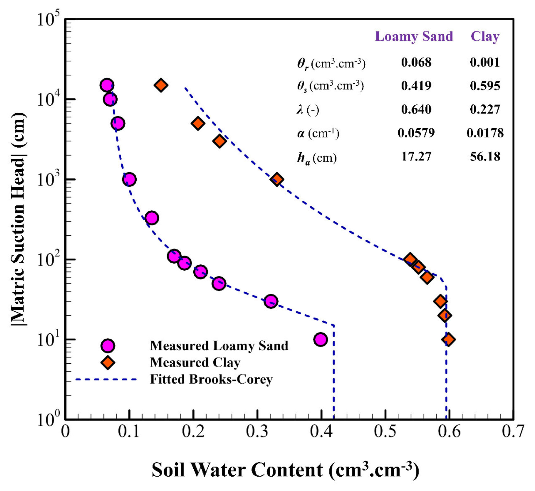
Figure 1. Fitting of laboratory SWRCs using the Brooks and Corey [36] model.
Hydrology 12 00164 g001
Figure 2. Fitting of laboratory SWRCs using the Visser [63] model.
Hydrology 12 00164 g002
Figure 3. Fitting of laboratory SWRCs using the Gardner [64] model.
Hydrology 12 00164 g003
Figure 4. Fitting of laboratory SWRCs using the King [62] and Gillham et al. [66] models.
Hydrology 12 00164 g004
Figure 5. Fitting of laboratory SWRCs using the van Genuchten models (m unconstrained, m = 1 − 1/n, and m = 1 − 2/n).
Hydrology 12 00164 g005
Figure 6. Fitting of laboratory SWRCs using the Tani [67] model.
Hydrology 12 00164 g006
Figure 7. Fitting of laboratory SWRCs using the Campbell [65] and Hutson–Cass [40] models.
Hydrology 12 00164 g007
Figure 8. Fitting of laboratory SWRCs using the Tani [67] and Russo [69] models.
Hydrology 12 00164 g008
Figure 9. Fitting of laboratory SWRCs using the Campbell and Shiozawa [42] model.
Hydrology 12 00164 g009
Figure 10. Fitting of laboratory SWRCs using the Fredlund and Xing [45] model.
Hydrology 12 00164 g010
Figure 11. Fitting of laboratory SWRCs using the van Genuchten and Brooks–Corey models corrected by Fayer and Simmons [47].
Hydrology 12 00164 g011
Figure 12. Fitting of laboratory SWRCs using the Aussoline et al. [49] model.
Hydrology 12 00164 g012
Figure 13. Fitting of laboratory SWRCs using the Khlosi et al. [52] model.
Hydrology 12 00164 g013
Figure 14. Fitting of laboratory SWRCs using the double-exponential Dexter et al. [54] model.
Hydrology 12 00164 g014
Figure 15. Fitting of laboratory SWRCs using the Kosugi lognormal and Romano bimodal lognormal models.
Hydrology 12 00164 g015
Table 1. Correlation matrix for estimated parameters of Visser’s model.
ClayLoamy Sand
abc ϕ abc ϕ
a1.00 1.00
b0.971.00 0.971.00
c−0.98−0.881.00 −1.00−0.971.00
ϕ 0.940.98−0.911.000.951.00−0.941.00
Table 2. Value, standard error (SE), and 95% confidence limits (CLs) of Visser’s model for clay and loamy sand soils.
ClayLoamy Sand
CL CL
ValueSELowerUpperValueSELowerUpper
a29.4212.04−4.0162.862.46110.39−252.10257.03
b0.010.21−0.580.612.98124.48−284.1290.04
c3.280.132.933.644.255.39−8.1816.69
ϕ 0.590.050.460.710.4411.58−26.2727.15
Table 3. Correlation matrix for estimated parameters of van Genuchten’s model considering m = 1 − 1/n and m as a variable parameter. It is worth noting that in heavy soils, θr may become negative, which is considered equal to zero.
m   =   1 1 / n
ClayLoamy Sand
θsαn θrθsαn
θs1.00 θr1.00
α0.711.00 θs−0.171.00
n−0.51−0.881.00 α−0.390.631.00
n0.67−0.37−0.861.00
Variable m
θsαnm θrθsαnm
θs1.00 θr1.00
α−0.211.00 θs0.081.00
n−0.620.821.00 α−0.63−0.061.00
m0.53−0.91−0.981.00n−0.42−0.470.771.00
m0.590.38−0.90−0.961.00
Table 4. Value, standard error (SE), and 95% confidence limits (CLs) of Russo’s model for clay and loamy sand soils.
ClayLoamy Sand
CL CL
ValueSELowerUpperValueSELowerUpper
θs0.590.020.550.630.440.020.400.48
θr0.200.020.160.240.090.010.070.11
β0.660.000.660.676.030.016.016.06
k1138.50801.57−756.923033.92793.1798.31566.471019.88
Table 5. Summary of the reviewed SWRC models.
YearModelParameters
1964Brooks and Corey θr, θs, α, λ
1965Kingθs, ho, b, ε, γ
1966Vissera, b, c, φ
1969Lalibertea, b, c, θr, θs, ha
1970Gardnera, b
1974Campbellθs, ha, b
1976Gillham et al.θs, ho, b, γ
1980van Genuchtenθr, θs, α, n, m
1982Taniθr, θs, hi
1984McKee and Bumbθr, θs, hi
1987Hutson and Cassθs, θi, α, b
1988Russoθr, θs, β, k
1988Vogel and Cislerovaθr, θm, α, n, m
1992Campbell and Shiozawaθa, ho, A, α, m
1994Shiozawa et al.a, b, c, α, n, m
1994Rossi and Nimmoθs, α, β, he, ho
1994Fredlund and Xingθs, a, n, m
1994Zhang and van Genuchtenθr, θs, C1, C2, δ
1994Kosugiθr, θs, ho, ha, n
1995Fayer and Simmons (FSVG)θa, θs, ho, α, n, m
1995Fayer and Simmons (FSBC)θa, θs, ho, α, λ
1996Kosugiθr, θs, ho, n
1998Assouline et al.θL, θs, hL, n, m
2000Webbk, hm, θm
2004Groenevelt and Grantθa, k0, k1, ha, n
2006Khlosi et al. (KCGS)θa, θs, ho, α, n
2006Ippisch et al.θr, θs, α, n, m, ha
2008Dexter et al.C, A1, A2, h1, h2
2009Omutoθr, θs, α1, α2, θ1
2010Groenevelt et al.θa, k0, k1, ha, n
2011Romano et al.θr, θs, w, α1, α2, n1, n2
2013Petersw, α, ho, n
2014Iden et al. (PDI)θr, θs, α, ho, n
2017Vanderlinden et al.A1, A2, h1, h2, k0, k1
2020Duθs, α, n, ho, λ
Disclaimer/Publisher’s Note: The statements, opinions and data contained in all publications are solely those of the individual author(s) and contributor(s) and not of MDPI and/or the editor(s). MDPI and/or the editor(s) disclaim responsibility for any injury to people or property resulting from any ideas, methods, instructions or products referred to in the content.