
Assessment of Baseflow Separation Methods Used in the Estimations of Design-Related Storm Hydrographs Across Various Return Periods


Abstract
1. Introduction
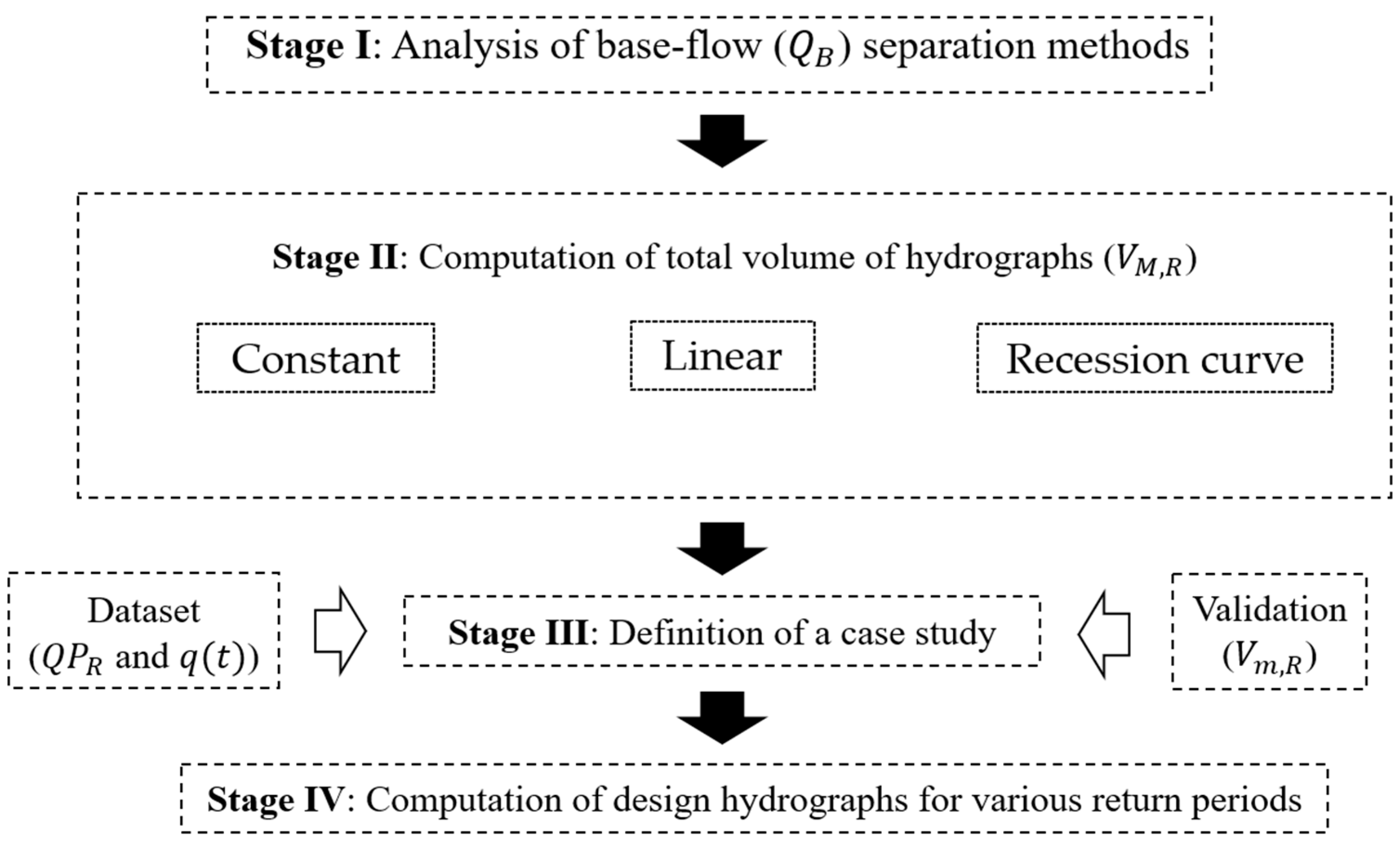
2. Methodology
2.1. Computation of Design-Related Hydrographs
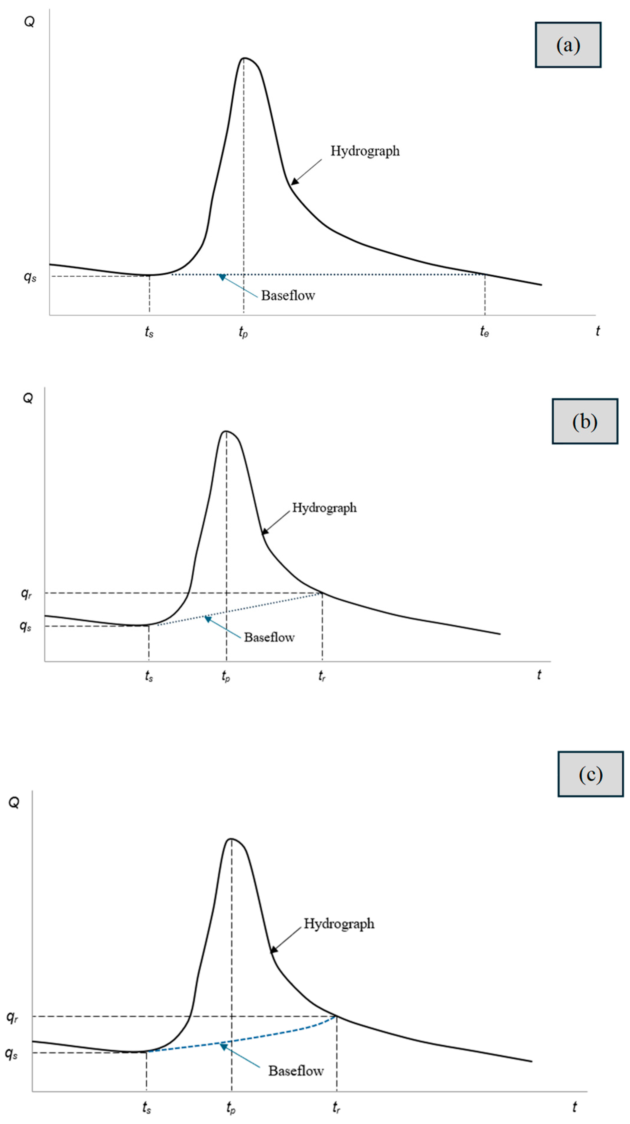
2.2. Baseflow Separation Methods and Hydrograph Volumes
2.2.1. Constant Baseflow
2.2.2. Linear Separation
2.2.3. Master Recession Curve
2.2.4. Other Baseflow Methods
- Boussinesq formula: This approach is derived from the governing equation for flow in saturated porous media. It provides a more physically based alternative to the empirical relationships described in Section 2.2.1, Section 2.2.2 and Section 2.2.3 and reduces the subjectivity typically associated with baseflow separation methods.
- Isotopic method: Certain water isotopes, such as oxygen-18 and deuterium, maintain stable isotopic compositions within specific components of the hydrological cycle, including aquifers and water bodies in which isotopic fractionation does not occur.
2.3. Summary of Baseflow Separation and Hydrograph Volumes
3. Practical Application
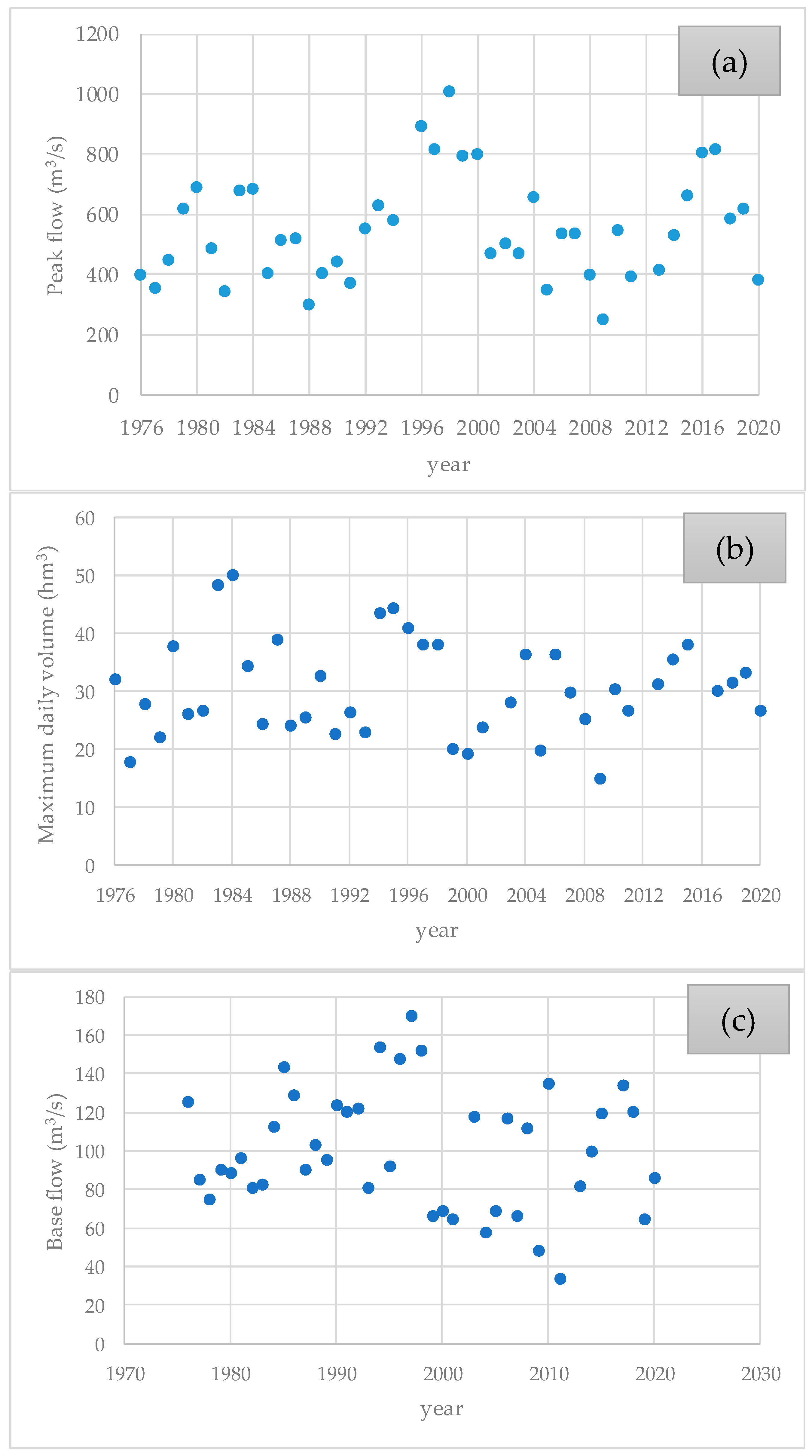
3.1. Case Study, Datasets, and Frequency Analysis
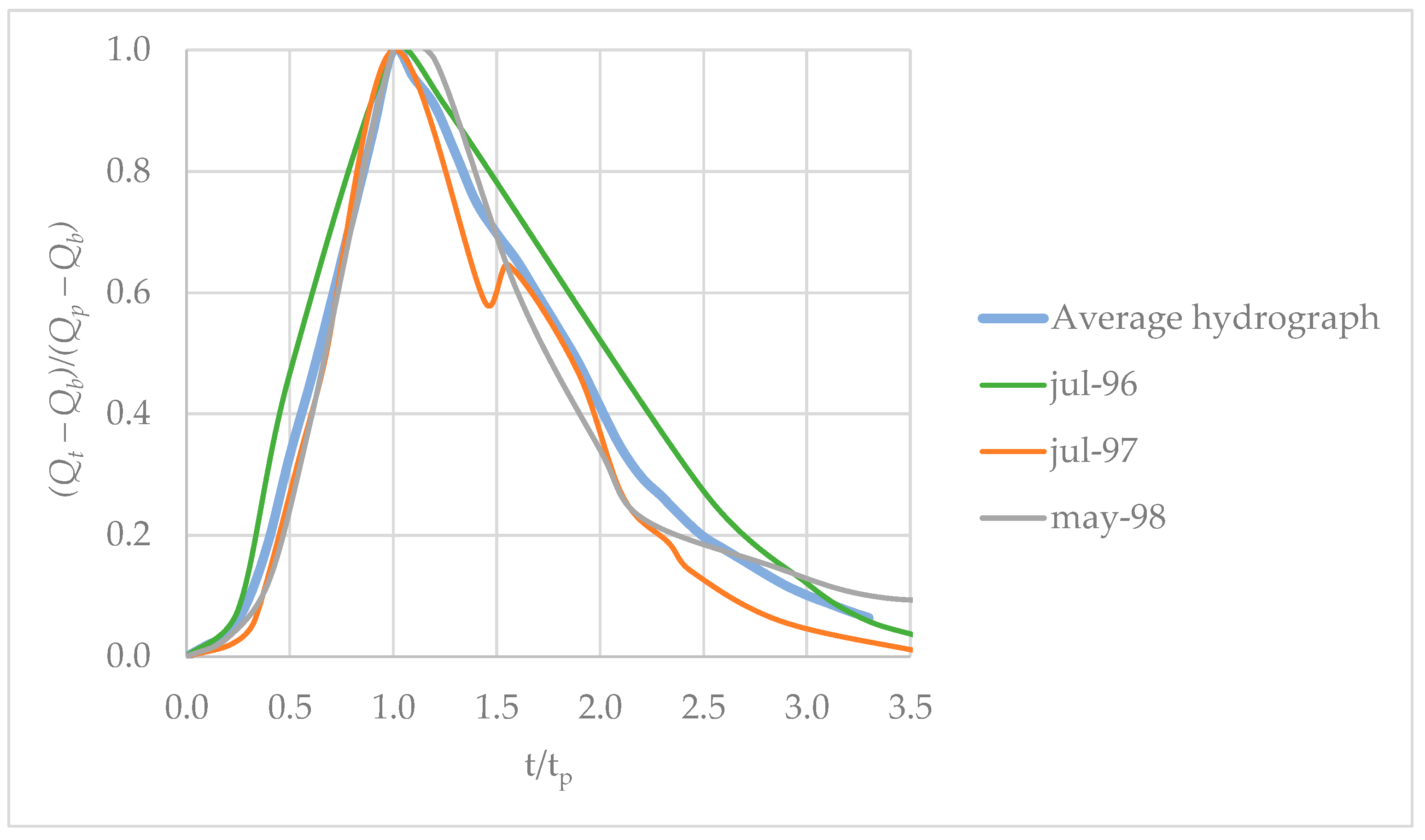
3.2. Computation of Design-Related Hydrographs
4. Discussion
4.1. Advantages and Limitations
4.2. Regional Analysis and Dataset Comparison
4.2.1. Regional Analysis for the Case Study
4.2.2. Comparison of an Additional Stream-Gauge Station
4.3. Application of the Boussinesq Formula and Isotopic Methods
5. Conclusions
- The frequency analysis demonstrated that the L-moments technique was the most effective approach in calculating peak flows, initial baseflows, and the maximum volume values of storm hydrographs for different return periods.
- The findings confirm that the statistical models used are well-suited for predicting events with return periods ranging from 5 to 200 years, as the proposed model successfully reproduces extreme values of peak flows, initial baseflows, and storm hydrograph volumes.
- The linear baseflow separation method provided the highest accuracy, with a root mean square error (RMSE) of 0.35% in terms of maximum volume across different return periods. However, the constant and master recession curve methods also yielded reliable results, with RMSE values of 3.02% and 2.92%, respectively. These results indicate that the proposed model is a valuable tool for hydrologists in computing storm hydrographs for different return periods.
Author Contributions
Funding
Data Availability Statement
Conflicts of Interest
Nomenclature
| Watershed area (km2) | |
| Parameters of the Boussinesq equation | |
| Aquifer width (m) | |
| Concentration sample | |
| Concentration of isotopes | |
| Baseflow volume (m3) | |
| Depth of an aquifer (m) | |
| Discharge of an aquifer (m3/s) | |
| Groundwater level (m) | |
| Decay exponent (s−1) | |
| Saturated hydraulic conductivity of the unconfined aquifer (m/s) | |
| Total length of contributing channels (m) | |
| Slope or factor of the linear baseflow method (m3/s/h) | |
| Number of analysed storm hydrographs (-) | |
| Baseflow discharge (m3/s) | |
| Total discharge of a storm hydrograph (m3/s) | |
| Peak flow (m3/s) | |
| Flow before and after a storm hydrograph (m3/s) | |
| Constant baseflow or initial baseflow discharge (m3/s) | |
| Final discharge of the baseflow function (m3/s) | |
| Drainage density (1/m) | |
| Root mean square error (%) | |
| Storm runoff volume (m3) | |
| Dimensionless hydrograph (-) | |
| Auxiliar variable for integration purposes | |
| Duration of a storm hydrograph (s) | |
| Time (s) | |
| Peak time (s) | |
| Initial time of a recorded hydrograph (s) | |
| / | Final time of a recorded hydrograph (s), where corresponds to a constant baseflow and corresponds to linear and recession curve methods |
| Total modelled volume (m3) | |
| Total measured volume (m3) | |
| Horizontal distance (m) | |
| Isotopic content (‰) | |
| Subscripts | |
| Refers to a return period (years) |
Appendix A. Demonstration of Additional Baseflow Methods
Appendix A.1. Based on the Boussinesq Equation
Appendix A.2. Isotopic Method
References
- Basso, S.; Merz, R.; Tarasova, L.; Miniussi, A. Extreme Flooding Controlled by Stream Network Organization and Flow Regime. Nat. Geosci. 2023, 16, 339–343. [Google Scholar] [CrossRef]
- Chikamori, H. Rainfall-Runoff Analysis of Flooding Caused by Typhoon RUSA in 2002 in the Gangneung Namdae River Basin, Korea. J. Nat. Disaster Sci. 2004, 26, 95–100. [Google Scholar]
- Crookston, B.M.; Erpicum, S. Hydraulic Engineering of Dams. J. Hydraul. Res. 2022, 60, 184–186. [Google Scholar] [CrossRef]
- Assaf, M.N.; Manenti, S.; Creaco, E.; Giudicianni, C.; Tamellini, L.; Todeschini, S. New Optimization Strategies for SWMM Modeling of Stormwater Quality Applications in Urban Area. J. Environ. Manag. 2024, 361, 121244. [Google Scholar] [CrossRef]
- Dotto, C.B.S.; Kleidorfer, M.; Deletic, A.; Fletcher, T.D.; McCarthy, D.T.; Rauch, W. Stormwater Quality Models: Performance and Sensitivity Analysis. Water Sci. Technol. 2010, 62, 837–843. [Google Scholar] [CrossRef]
- Chow, V.T.; Maidment, D.R.; Mays, L.W. Applied Hydrology; McGraw-Hill International Editions: New York, NY, USA, 1988; ISBN 0-07-010810-2. [Google Scholar]
- Ross, C.A.; Ali, G.; Bansah, S.; Laing, J.R. Evaluating the Relative Importance of Shallow Subsurface Flow in a Prairie Landscape. Vadose Zone J. 2017, 16, 1–20. [Google Scholar] [CrossRef]
- Bronstert, A.; Niehoff, D.; Schiffler, G.R. Modelling Infiltration and Infiltration Excess: The Importance of Fast and Local Processes. Hydrol. Process. 2023, 37, e14875. [Google Scholar] [CrossRef]
- Barthel, R.; Banzhaf, S. Groundwater and Surface Water Interaction at the Regional-Scale—A Review with Focus on Regional Integrated Models. Water Resour. Manag. 2016, 30, 1–32. [Google Scholar] [CrossRef]
- Nogueira, G.E.H.; Partington, D.; Heidbüchel, I.; Fleckenstein, J.H. Combined Effects of Geological Heterogeneity and Discharge Events on Groundwater and Surface Water Mixing. J. Hydrol. 2024, 638, 131467. [Google Scholar] [CrossRef]
- Aranguren-Díaz, Y.; Galán-Freyle, N.J.; Guerra, A.; Manares-Romero, A.; Pacheco-Londoño, L.C.; Romero-Coronado, A.; Vidal-Figueroa, N.; Machado-Sierra, E. Aquifers and Groundwater: Challenges and Opportunities in Water Resource Management in Colombia. Water 2024, 16, 685. [Google Scholar] [CrossRef]
- Briggs, M.A.; Newman, C.; Benton, J.R.; Rey, D.M.; Konrad, C.P.; Ouellet, V.; Torgersen, C.E.; Gruhn, L.; Fleming, B.J.; Gazoorian, C.; et al. James Buttle Review: The Characteristics of Baseflow Resilience Across Diverse Ecohydrological Terrains. Hydrol. Process. 2025, 39, e70101. [Google Scholar] [CrossRef]
- Baig, F.; Sherif, M.; Faiz, M.A. Quantification of Precipitation and Evapotranspiration Uncertainty in Rainfall-Runoff Modeling. Hydrology 2022, 9, 51. [Google Scholar] [CrossRef]
- Jehanzaib, M.; Ajmal, M.; Achite, M.; Kim, T.-W. Comprehensive Review: Advancements in Rainfall-Runoff Modelling for Flood Mitigation. Climate 2022, 10, 147. [Google Scholar] [CrossRef]
- Rivera Trejo, F.; Escalante Sandoval, C. Análisis Comparativo de Técnicas de Estimación de Avenidas de Diseño. Ing. Del Agua 1999, 6, 49–54. [Google Scholar] [CrossRef]
- Coronado-Hernández, O.E.; Fuertes-Miquel, V.S.; Arrieta-Pastrana, A. The Development of a Hydrological Method for Computing Extreme Hydrographs in Engineering Dam Projects. Hydrology 2024, 11, 194. [Google Scholar] [CrossRef]
- Shin, M.-J.; Kim, C.-S. Analysis of the Effect of Uncertainty in Rainfall-Runoff Models on Simulation Results Using a Simple Uncertainty-Screening Method. Water 2019, 11, 1361. [Google Scholar] [CrossRef]
- Dotson, H.W. Watershed Modeling with HEC-HMS (Hydrologic Engineering Centers-Hydrologic Modeling System) Using Spatially Distributed Rainfall. In Coping with Flash Floods; Springer: Berlin/Heidelberg, Germany, 2001; pp. 219–230. [Google Scholar]
- Ma, L.; He, C.; Bian, H.; Sheng, L. MIKE SHE Modeling of Ecohydrological Processes: Merits, Applications, and Challenges. Ecol. Eng. 2016, 96, 137–149. [Google Scholar] [CrossRef]
- Swain, S.; Mishra, S.K.; Pandey, A.; Pandey, A.C.; Jain, A.; Chauhan, S.K.; Badoni, A.K. Hydrological Modelling through SWAT over a Himalayan Catchment Using High-Resolution Geospatial Inputs. Environ. Chall. 2022, 8, 100579. [Google Scholar] [CrossRef]
- Hodges, B.R.; Sharior, S.; Tiernan, E.D.; Jenkins, E.; Riaño-Briceño, G.; Davila-Hernandez, C.; Madadi-Kandjani, E.; Yu, C.-W. Introducing SWMM5+. J. Environ. Eng. 2024, 150, 02524003. [Google Scholar] [CrossRef]
- Campisano, A.; Catania, F.V.; Modica, C. Evaluating the SWMM LID Editor Rain Barrel Option for the Estimation of Retention Potential of Rainwater Harvesting Systems. Urban Water J. 2017, 14, 876–881. [Google Scholar] [CrossRef]
- Quintero, F.; Velásquez, N. Implementation of TETIS Hydrologic Model into the Hillslope Link Model Framework. Water 2022, 14, 2610. [Google Scholar] [CrossRef]
- Duncan, H.P. Baseflow Separation—A Practical Approach. J. Hydrol. 2019, 575, 308–313. [Google Scholar] [CrossRef]
- Szilagyi, J.; Parlange, M.B. Baseflow Separation Based on Analytical Solutions of the Boussinesq Equation. J. Hydrol. 1998, 204, 251–260. [Google Scholar] [CrossRef]
- International Atomic Energy Environmental Isotopes in the Hydrological Cycle: Principles and Applications, v. II: Atmospheric Water. 2001. Available online: https://unesdoc.unesco.org/ark:/48223/pf0000149442 (accessed on 15 May 2025).
- Yang, H.; Choi, H.T.; Lim, H. Applicability Assessment of Estimation Methods for Baseflow Recession Constants in Small Forest Catchments. Water 2018, 10, 1074. [Google Scholar] [CrossRef]
- Brutsaert, W.; Nieber, J.L. Regionalized Drought Flow Hydrographs from a Mature Glaciated Plateau. Water Resour. Res. 1977, 13, 637–643. [Google Scholar] [CrossRef]
- Gómez, S.; Guzmán, J. Separation of Base Flow in Upper Part of the Lebrija River Basin. Rev. Fac. Ing. Univ. Antioq. 2011, 61, 41–52. [Google Scholar] [CrossRef]
- Villalba-Barrios, A.F.; Coronado-Hernández, O.E.; Fuertes-Miquel, V.S.; Coronado-Hernández, J.R.; Ramos, H.M. Statistical Approach for Computing Base Flow Rates in Gaged Rivers and Hydropower Effect Analysis. Hydrology 2023, 10, 137. [Google Scholar] [CrossRef]
- Chen, X.; Shao, Q.; Xu, C.Y.; Zhang, J.; Zhang, L.; Ye, C. Comparative Study on the Selection Criteria for Fitting Flood Frequency Distribution Models with Emphasis on Upper-Tail Behavior. Water 2017, 9, 320. [Google Scholar] [CrossRef]
- Anghel, C.G. Revisiting the Use of the Gumbel Distribution: A Comprehensive Statistical Analysis Regarding Modeling Extremes and Rare Events. Mathematics 2024, 12, 2466. [Google Scholar] [CrossRef]
- Coronado-Hernández, O.E. Consideraciones de Incertidumbre en la Estimación de Hidrogramas de Diseño de Estructuras de Desviación y Rebosaderos en Presas. Master’s Dissertation, Universidad de los Andes, Bogotá, Colombia, 2010. [Google Scholar]


| Baseflow Method | Variable | Equation * |
|---|---|---|
| Constant | ||
| Linear | ||
| Master recession curve method | ||
| Boussinesq equation ** | ||
| Isotopic ** | ||
| Station Name | Station Code | Dataset Available | Latitude, Longitude |
|---|---|---|---|
| Páez | 35087020 | 1976–2020 | 5.08, −73.07 |
| San Agustín | 35087010 | 1961–2021 | 4.86, −73.23 |
| Casa de Máquinas | 35087070 | 1982, 1999 | 4.90, −73.23 |
| Chapasía | 35087060 | 1999–2024 | 5.16, −73.09 |
| Distribution | Statistical Tests | ||
|---|---|---|---|
| Kolmogorov-Smirnov | Chi-Square | Anderson-Darling | |
| Peak Flow series | |||
| Pearson III (PM) | 0.075 | 3.326 | 0.244 |
| Generalized Extreme Value (PM) | 0.077 | 3.326 | 0.240 |
| Gumbel (PM) | 0.085 | 1.837 | 0.265 |
| Pearson III (LM) | 0.066 | 2.953 | 0.189 |
| Gumbel (LM) | 0.070 | 2.581 | 0.202 |
| Generalized Extreme Value (LM) | 0.071 | 2.953 | 0.201 |
| Pearson III (MLE) | 0.071 | 2.953 | 0.197 |
| Gumbel (MLE) | 0.075 | 2.581 | 0.213 |
| Generalized Extreme Value (MLE) | 0.080 | 2.581 | 0.233 |
| Daily volume series | |||
| Generalized Extreme Value (PM) | 0.080 | 3.333 | 0.147 |
| Gumbel (PM) | 0.082 | 4.476 | 0.319 |
| Pearson III (PM) | 0.083 | 3.333 | 0.162 |
| Generalized Extreme Value (LM) | 0.072 | 3.714 | 0.135 |
| Pearson III (LM) | 0.072 | 4.476 | 0.137 |
| Gumbel (LM) | 0.074 | 3.333 | 0.219 |
| Gumbel (MLE) | 0.063 | 4.857 | 0.181 |
| Pearson III (MLE) | 0.074 | 5.238 | 0.146 |
| Generalized Extreme Value (MLE) | 0.081 | 2.571 | 0.161 |
| Baseflow series | |||
| Generalized Extreme Value (PM) | 0.085 | 4.857 | 0.236 |
| Pearson III (PM) | 0.088 | 3.333 | 0.272 |
| Gumbel (PM) | 0.132 | 10.571 | 0.666 |
| Generalized Extreme Value (LM) | 0.085 | 4.857 | 0.229 |
| Pearson III (LM) | 0.088 | 4.857 | 0.247 |
| Gumbel (LM) | 0.123 | 5.238 | 0.490 |
| Generalized Extreme Value (MLE) | 0.087 | 3.333 | 0.266 |
| Pearson III (MLE) | 0.094 | 3.333 | 0.276 |
| Gumbel (MLE) | 0.100 | 2.571 | 0.381 |
| Return Period (Years) | Estimated Volume (hm3) * | Computed Volume (hm3) ** | |||
|---|---|---|---|---|---|
| Constant | Linear | Master Recession Curve | |||
| 1 | 200 | 56.4 | 57.7 | 56.5 | 58.2 |
| 2 | 100 | 53.5 | 54.0 | 53.4 | 54.4 |
| 3 | 50 | 50.4 | 50.2 | 50.2 | 50.5 |
| 4 | 20 | 45.8 | 44.7 | 45.6 | 45.0 |
| 5 | 10 | 41.8 | 40.3 | 41.7 | 40.5 |
| 6 | 5 | 37.3 | 35.3 | 37.5 | 35.4 |
| = 6 | RMSE (%) | 3.02 | 0.35 | 2.92 | |
| Distribution | Statistical Tests | ||
|---|---|---|---|
| Kolmogorov–Smirnov | Chi-Square | Anderson–Darling | |
| Chapasía station | |||
| Pearson III (PM) | 0.093 | NaN * | 0.271 |
| Generalized Extreme Value (PM) | 0.105 | NaN | 0.295 |
| Gumbel (PM) | 0.126 | 0.909 | 0.487 |
| Generalized Extreme Value (LM) | 0.090 | NaN | 0.162 |
| Pearson III (LM) | 0.109 | NaN | 0.070 |
| Gumbel (LM) | 0.127 | 0.909 | 0.424 |
| Generalized Extreme Value (MLE) | 0.085 | NaN | 0.159 |
| Gumbel (MLE) | 0.109 | 0.909 | 0.344 |
| Pearson III (MLE) | 0.377 | NaN | 4.195 |
| San Agustín station | |||
| Generalized Extreme Value (PM) | 0.125 | 16.526 | 0.73 |
| Pearson III (PM) | 0.127 | 15.368 | 0.77 |
| Gumbel (PM) | 0.139 | 15.754 | 1.027 |
| Pearson III (LM) | 0.119 | 13.439 | 0.695 |
| Gumbel (LM) | 0.121 | 10.737 | 0.812 |
| Generalized Extreme Value (LM) | 0.121 | 13.053 | 0.71 |
| Gumbel (MLE) | 0.115 | 11.509 | 0.723 |
| Pearson III (MLE) | 0.126 | 14.982 | 0.747 |
| Generalized Extreme Value (MLE) | 0.13 | 12.281 | 0.784 |
| i | Return Period (Years) | Estimated Volume (hm3) | Computed Volume (hm3) |
|---|---|---|---|
| 1 | 200 | 322.02 | 319.0 |
| 2 | 100 | 298.69 | 295.4 |
| 3 | 50 | 276.23 | 271.7 |
| 4 | 20 | 240.91 | 240.1 |
| 5 | 10 | 222.05 | 215.7 |
| 6 | 5 | 196.69 | 190.3 |
| = 6 | RMSE (%) | 1.98% | |
Disclaimer/Publisher’s Note: The statements, opinions and data contained in all publications are solely those of the individual author(s) and contributor(s) and not of MDPI and/or the editor(s). MDPI and/or the editor(s) disclaim responsibility for any injury to people or property resulting from any ideas, methods, instructions or products referred to in the content. |
© 2025 by the authors. Licensee MDPI, Basel, Switzerland. This article is an open access article distributed under the terms and conditions of the Creative Commons Attribution (CC BY) license (https://creativecommons.org/licenses/by/4.0/).
Share and Cite
Coronado-Hernández, O.E.; Méndez-Anillo, R.D.; Saba, M. Assessment of Baseflow Separation Methods Used in the Estimations of Design-Related Storm Hydrographs Across Various Return Periods. Hydrology 2025, 12, 158. https://doi.org/10.3390/hydrology12060158
Coronado-Hernández OE, Méndez-Anillo RD, Saba M. Assessment of Baseflow Separation Methods Used in the Estimations of Design-Related Storm Hydrographs Across Various Return Periods. Hydrology. 2025; 12(6):158. https://doi.org/10.3390/hydrology12060158
Chicago/Turabian StyleCoronado-Hernández, Oscar E., Rafael D. Méndez-Anillo, and Manuel Saba. 2025. "Assessment of Baseflow Separation Methods Used in the Estimations of Design-Related Storm Hydrographs Across Various Return Periods" Hydrology 12, no. 6: 158. https://doi.org/10.3390/hydrology12060158
APA StyleCoronado-Hernández, O. E., Méndez-Anillo, R. D., & Saba, M. (2025). Assessment of Baseflow Separation Methods Used in the Estimations of Design-Related Storm Hydrographs Across Various Return Periods. Hydrology, 12(6), 158. https://doi.org/10.3390/hydrology12060158