
Extraction of Major Groundwater Ions from Total Dissolved Solids and Mineralization Using Artificial Neural Networks: A Case Study of the Aflou Syncline Region, Algeria
 ,
,  and
and 
Abstract
1. Introduction
2. Materials
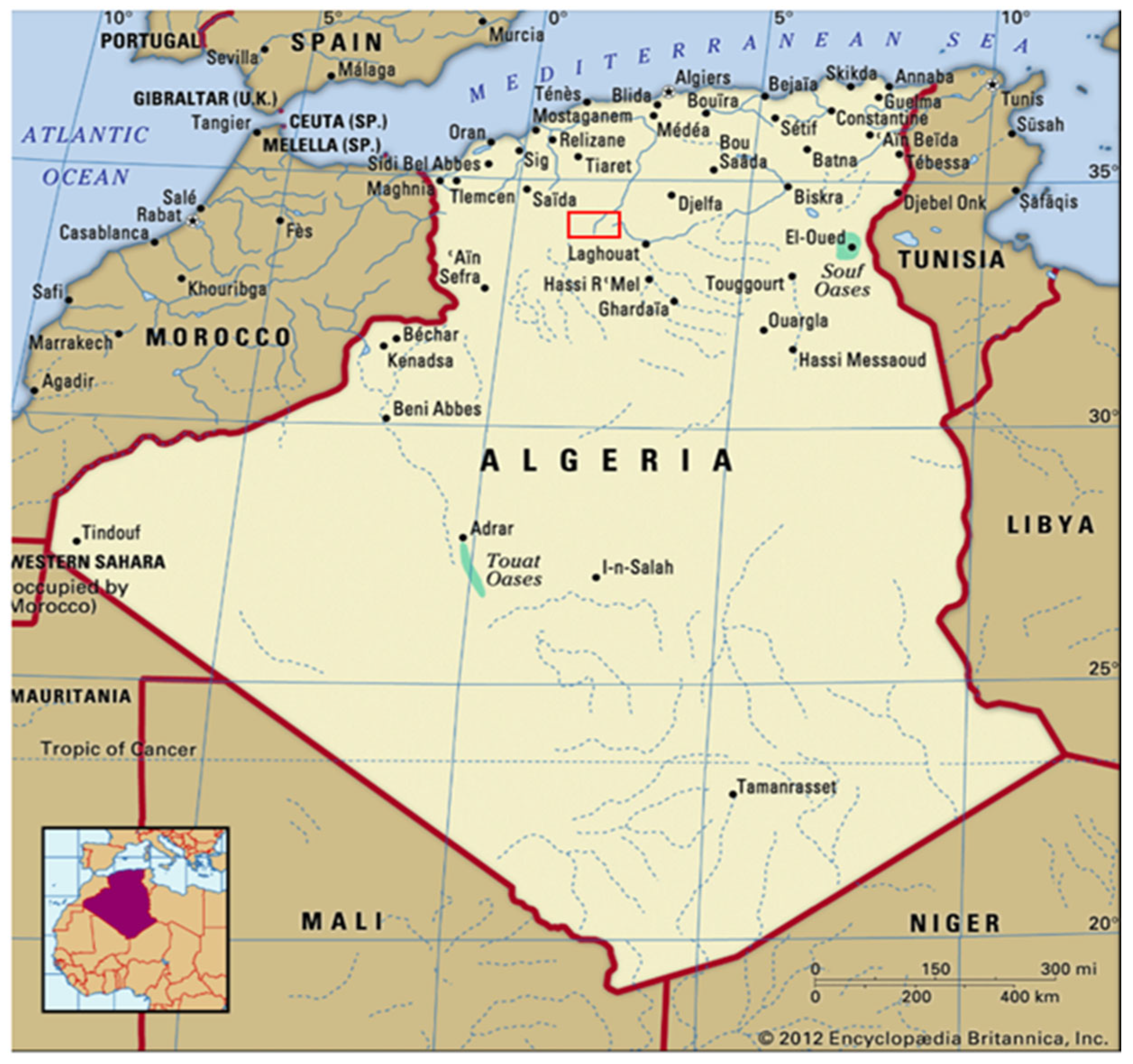
2.1. Study Area and Data Collection
2.2. Mineralization
2.2.1. Laboratory Procedure
2.2.2. The Conversion Factor Method
3. Methodology
3.1. Artificial Neural Networks and Optimization Algorithms
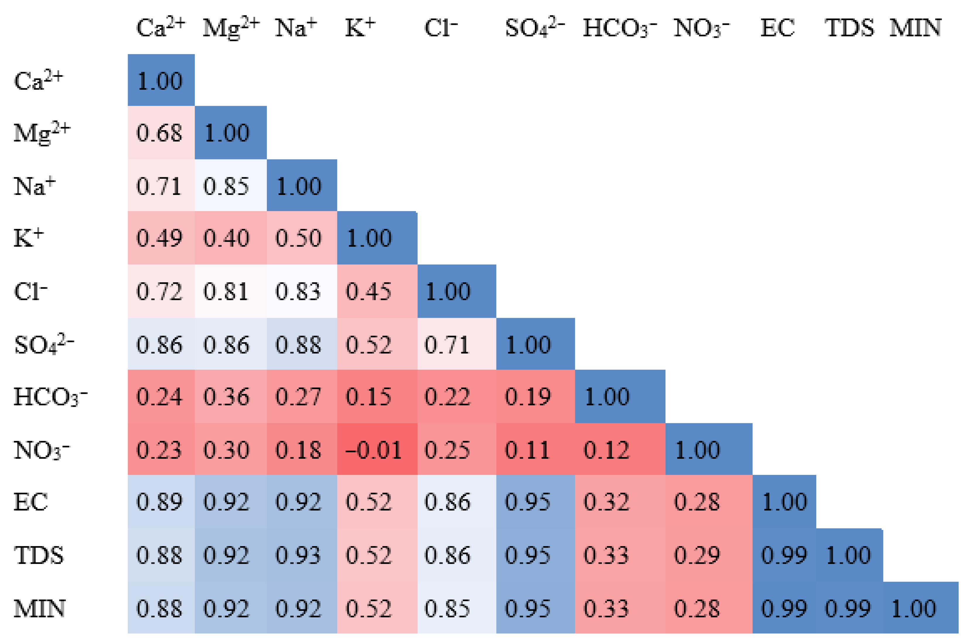
3.2. Model Development
3.3. Measures of Accuracy
3.4. Hyperparameters Selection
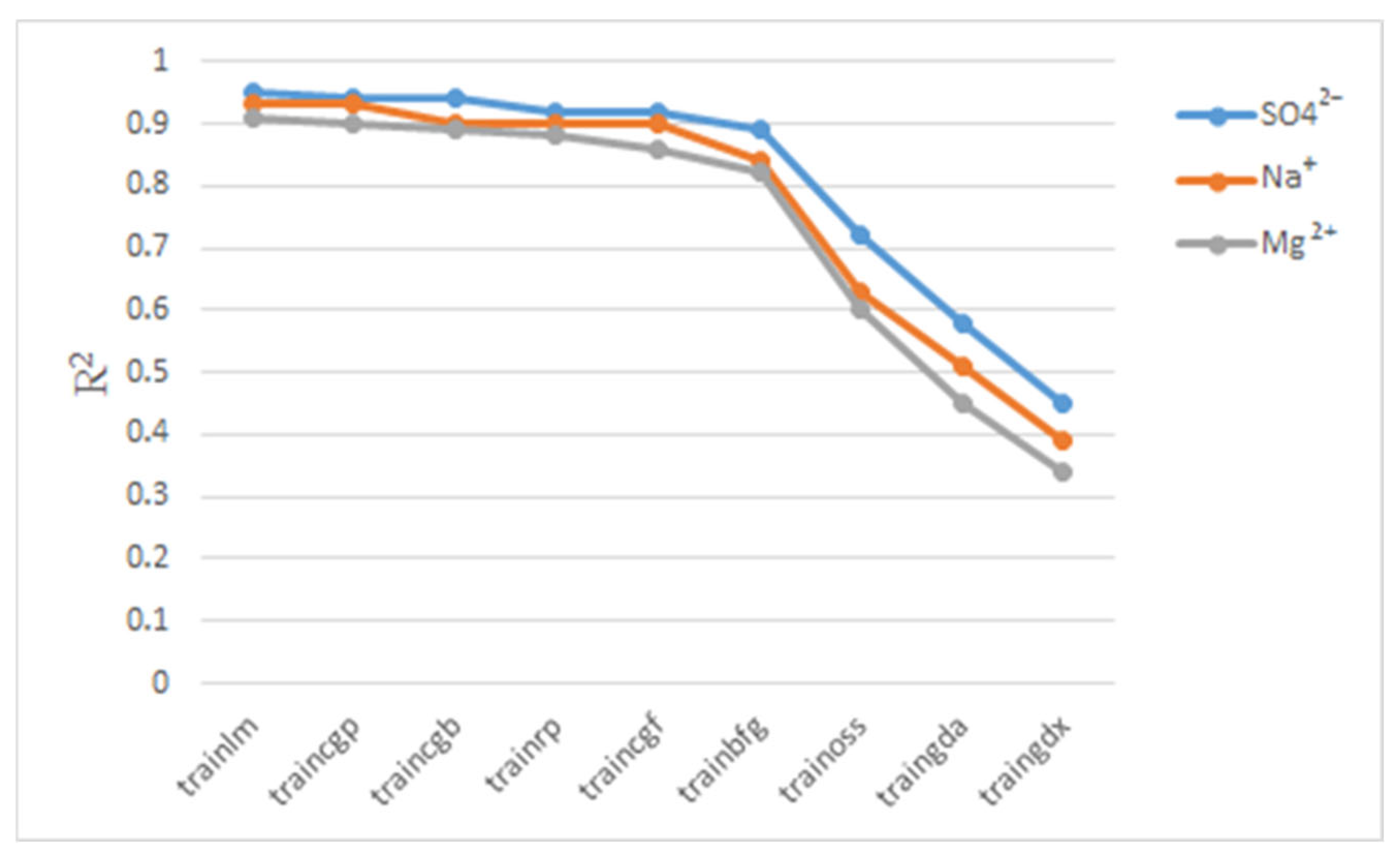
4. Results and Discussion
5. Conclusions
Author Contributions
Funding
Data Availability Statement
Conflicts of Interest
Abbreviations
| TDS | Total dissolved solids |
| MIN | Mineralization |
| MLP | Multilayer perceptron |
| LMBP | Levenberg–Marquardt backpropagation |
| AI | Artificial intelligence |
| WQI | Water quality index |
| ANN | Artificial neural networks |
| EC | Electrical conductivity |
| RBF-NN | Radial basis function neural networks |
| PNN | Probabilistic neural networks |
| FCNN | Feedforward connected neural networks |
| R2 | Coefficient of determination |
| RMSE | Root mean square error |
| CB | Charge balance |
| LMBP-MLP | Levenberg–Marquardt backpropagation multilayer perceptron |
References
- UNESCO. The United Nations World Water Development Report 2018-Nature-Based Solutions for Water; UN: New York, NY, USA, 2019. [Google Scholar]
- Boretti, A.; Rosa, L. Reassessing the projections of the world water development report. NPJ Clean Water 2019, 2, 15. [Google Scholar] [CrossRef]
- Canton, H. Food and agriculture organization of the United Nations—FAO. In The Europa Directory of International Organizations 2021; Routledge: Oxfordshire, UK, 2021; pp. 297–305. [Google Scholar]
- Hamed, Y.; Hadji, R.; Redhaounia, B.; Zighmi, K.; Bâali, F.; El Gayar, A. Climate impact on surface and groundwater in North Africa: A global synthesis of findings and recommendations. Euro-Mediterr. J. Environ. Integr. 2018, 3, 25. [Google Scholar] [CrossRef]
- Bioud, I.; Semar, A.; Laribi, A.; Douaibia, S.; Chabaca, M.N. Assessment of groundwater quality and its suitability for irrigation: The case of Souf Valley phreatic aquifer. Alger. J. Environ. Sci. Technol. 2023, 9, 1429–1441. [Google Scholar]
- Shiri, N.; Shiri, J.; Yaseen, Z.M.; Kim, S.; Chung, I.M.; Nourani, V.; Zounemat-Kermani, M. Development of artificial intelligence models for well groundwater quality simulation: Different modeling scenarios. PLoS ONE 2021, 16, e0251510. [Google Scholar] [CrossRef]
- Alizamir, M.; Ahmed, K.O.; Kim, S.; Heddam, S.; Gorgij, A.D.; Chang, S.W. Development of a robust daily soil temperature estimation in semi-arid continental climate using meteorological predictors based on computational intelligent paradigms. PLoS ONE 2023, 18, e0293751. [Google Scholar] [CrossRef]
- Lopes, M.B.S. The 2017 World Health Organization classification of tumors of the pituitary gland: A summary. Acta Neuropathol. 2017, 134, 521–535. [Google Scholar] [CrossRef]
- Khadra, F.W.; El Sibai, R.; Khadra, W.M. Deriving groundwater major ions from electrical conductivity using artificial neural networks supported by analytical hydrochemical solutions. Groundw. Sustain. Dev. 2024, 24, 101056. [Google Scholar] [CrossRef]
- Tao, H.; Hameed, M.M.; Marhoon, H.A.; Zounemat-Kermani, M.; Heddam, S.; Kim, S.; Sulaiman, S.O.; Tan, M.L.; Sa’adi, Z.; Mehr, A.D.; et al. Groundwater level prediction using machine learning models: A comprehensive review. Neurocomputing 2022, 489, 271–308. [Google Scholar] [CrossRef]
- Khudair, B.H.; Jasim, M.M.; Alsaqqar, A.S. Artificial neural network model for the prediction of groundwater quality. Civ. Eng. J. 2018, 4, 2959–2970. [Google Scholar] [CrossRef]
- Setshedi, K.J.; Mutingwende, N.; Ngqwala, N.P. The use of artificial neural networks to predict the physicochemical characteristics of water quality in three district municipalities, eastern cape province, South Africa. Int. J. Environ. Res. Public Health 2021, 18, 5248. [Google Scholar] [CrossRef]
- Stylianoudaki, C.; Trichakis, I.; Karatzas, G.P. Modeling groundwater nitrate contamination using artificial neural networks. Water 2022, 14, 1173. [Google Scholar] [CrossRef]
- Allawi, M.F.; Al-Ani, Y.; Jalal, A.D.; Ismael, Z.M.; Sherif, M.; El-Shafie, A. Groundwater quality parameters prediction based on data-driven models. Eng. Appl. Comput. Fluid Mech. 2024, 18, 2364749. [Google Scholar] [CrossRef]
- Mateo, L.F.; Más-López, M.I.; García-del-Toro, E.M.; García-Salgado, S.; Quijano, M.Á. Artificial Neural Networks to Predict Electrical Conductivity of Groundwater for Irrigation Management: Case of Campo de Cartagena (Murcia, Spain). Agronomy 2024, 14, 524. [Google Scholar] [CrossRef]
- Al-Sulttani, A.O.; Ali, S.K.; Abdulhameed, A.A.; Jassim, D.T. Artificial Neural Network Assessment of Groundwater Quality for Agricultural Use in Babylon City: An Evaluation of Salinity and Ionic Composition. Int. J. Des. Nat. Ecodyn. 2024, 19, 329–336. [Google Scholar] [CrossRef]
- Sekkoum, M.; Safa, A.; Stamboul, M. Groundwater hydrochemistry of Aflou syncline, Central Saharan Atlas of Algeria. Desalin. Water Treat. 2020, 190, 424–439. [Google Scholar] [CrossRef]
- Cerlini, P.B.; Silvestri, L.; Meniconi, S.; Brunone, B. Simulation of the water table elevation in shallow unconfined aquifers by means of the ERA5 soil moisture dataset: The Umbria region case study. Earth Interact. 2021, 25, 15–32. [Google Scholar] [CrossRef]
- Kim, S.; Cho, J.S.; Park, J.K. Hydrological analysis using the neural networks in the parallel reservoir groups, South Korea. In World Water & Environmental Resources Congress; American Society of Civil Engineers: Reston, VA, USA, 2003. [Google Scholar]
- Kim, S.; Seo, Y.; Lee, C.J. Modeling of rainfall by combining neural computation and wavelet technique. Procedia Eng. 2016, 154, 1231–1236. [Google Scholar] [CrossRef]
- Zakhrouf, M.; Bouchelkia, H.; Stamboul, M.; Kim, S.; Heddam, S. Time series forecasting of river flow using an integrated approach of wavelet multi-resolution analysis and evolutionary data-driven models. A Case Study: Sebaou River (Algeria). Phys. Geogr. 2018, 39, 506–522. [Google Scholar] [CrossRef]
- Hagan, M.T.; Demuth, H.B.; Beale, M. Neural Network Design; PWS Publishing Co., Ltd.: Worcester, UK, 1997. [Google Scholar]
- Haykin, S. Neural Networks: A Comprehensive Foundation; Prentice-Hall Inc.: Upper Saddle River, NJ, USA, 1999. [Google Scholar]
- Kim, S.; Lee, S. Forecasting of flood stage using neural networks in the Nakdong river, South Korea. In Watershed Management and Operations Management; American Society of Civil Engineers: Reston, VA, USA, 2000. [Google Scholar]
- Bishop, C.M.; Nasrabadi, N.M. Pattern Recognition and Machine Learning; Springer: New York, NY, USA, 2006. [Google Scholar]
- Zakhrouf, M.; Bouchelkia, H.; Stamboul, M.; Kim, S.; Singh, V.P. Implementation on the evolutionary machine learning approaches for streamflow forecasting: Case study in the Seybous River, Algeria. J. Korea Water Resour. Assoc. 2020, 53, 395–408. [Google Scholar]
- Rumelhart, D.E.; Hinton, G.E.; Williams, R.J. Learning representations by back-propagating errors. Nature 1986, 323, 533–536. [Google Scholar] [CrossRef]
- Nocedal, J.; Wright, S.J. Numerical Optimization; Springer: New York, NY, USA, 1999. [Google Scholar]
- Elmeddahi, Y.; Ragab, R. Prediction of the groundwater quality index through machine learning in Western Middle Cheliff plain in North Algeria. Acta Geophys. 2022, 70, 1797–1814. [Google Scholar] [CrossRef]
- Ahlgren, P.; Jarneving, B.; Rousseau, R. Requirements for a cocitation similarity measure, with special reference to Pearson’s correlation coefficient. JASIST 2003, 54, 550–560. [Google Scholar] [CrossRef]
- Kim, S.; Seo, Y.; Malik, A.; Kim, S.; Heddam, S.; Yaseen, Z.M.; Kisi, O.; Singh, V.P. Quantification of river total phosphorus using integrative artificial intelligence models. Ecol. Indic. 2023, 153, 110437. [Google Scholar] [CrossRef]
- Seo, Y.; Kim, S.; Singh, V.P. Physical interpretation of river stage forecasting using soft computing and optimization algorithms. In Harmony Search Algorithm: Proceedings of the 2nd International Conference on Harmony Search Algorithm (ICHSA2015); Springer: Berlin/Heidelberg, Germany, 2016; pp. 259–266. [Google Scholar]
- Alizamir, M.; Gholampour, A.; Kim, S.; Keshtegar, B.; Jung, W.T. Designing a reliable machine learning system for accurately estimating the ultimate condition of FRP-confined concrete. Sci. Rep. 2024, 14, 20466. [Google Scholar] [CrossRef]
- Nash, J.E.; Sutcliffe, J.V. River flow forecasting through conceptual models part I—A discussion of principles. J. Hydrol. 1970, 10, 282–290. [Google Scholar] [CrossRef]
- Kim, S.; Singh, V.P.; Lee, C.J.; Seo, Y. Modeling the physical dynamics of daily dew point temperature using soft computing techniques. KSCE J. Civ. Eng. 2015, 19, 1930–1940. [Google Scholar] [CrossRef]
- Reed, M.H. Calculation of multicomponent chemical equilibria and reaction processes in systems involving minerals, gases and an aqueous phase. Geochim. Cosmochim. Acta 1982, 46, 513–528. [Google Scholar] [CrossRef]
- Stuyfzand, P.J. Hydrogeochemcal (HGC 2.1), for Storage, Management, Control, Correction and Interpretation of Water Quality Data in Excel® Spread Sheet; KWR-Rapport B111698-002; KWR: Nieuwegein, The Netherlands, 2012. [Google Scholar]
- Kim, S.; Kim, H.S. Uncertainty reduction of the flood stage forecasting using neural networks model. JAWRA J. Am. Water Resour. Assoc. 2008, 44, 148–165. [Google Scholar] [CrossRef]
- Fushiki, T. Estimation of prediction error by using K-fold cross-validation. Stat. Comput. 2011, 21, 137–146. [Google Scholar] [CrossRef]
- Gu, Y.; Wylie, B.K.; Boyte, S.P.; Picotte, J.; Howard, D.M.; Smith, K.; Nelson, K.J. An optimal sample data usage strategy to minimize overfitting and underfitting effects in regression tree models based on remotely-sensed data. Remote Sens. 2016, 8, 943. [Google Scholar] [CrossRef]
- Kisi, O.; Alizamir, M.; Trajkovic, S.; Shiri, J.; Kim, S. Solar radiation estimation in Mediterranean climate by weather variables using a novel Bayesian model averaging and machine learning methods. Neural Process. Lett. 2020, 52, 2297–2318. [Google Scholar] [CrossRef]


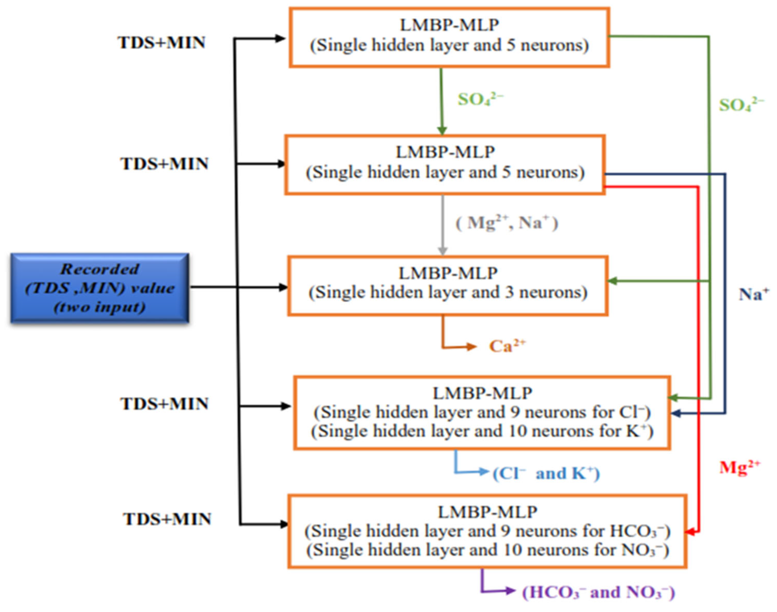
| ANN Model | Features | Output |
|---|---|---|
| LMBP-MLP1 | TDS, MIN | SO42− |
| LMBP-MLP2 | TDS, MIN, SO42− | Mg2+ |
| LMBP-MLP3 | TDS, MIN, SO42− | Na+ |
| LMBP-MLP4 | TDS, MIN, SO42−, Na+, Mg2+ | Ca2+ |
| LMBP-MLP5 | TDS, MIN, SO42−, Na+ | Cl− |
| LMBP-MLP6 | TDS, MIN, SO42−, Na+ | K+ |
| LMBP-MLP7 | TDS, MIN, Mg2+ | HCO3− |
| LMBP-MLP8 | TDS, MIN, Mg2+ | NO3− |
| ANN Model | Output | Training | Validation | Test | All | ||||||||
|---|---|---|---|---|---|---|---|---|---|---|---|---|---|
| R2 | RMSE (mg/L) | NSE | R2 | RMSE (mg/L) | NSE | R2 | RMSE (mg/L) | NSE | R2 | RMSE (mg/L) | NSE | ||
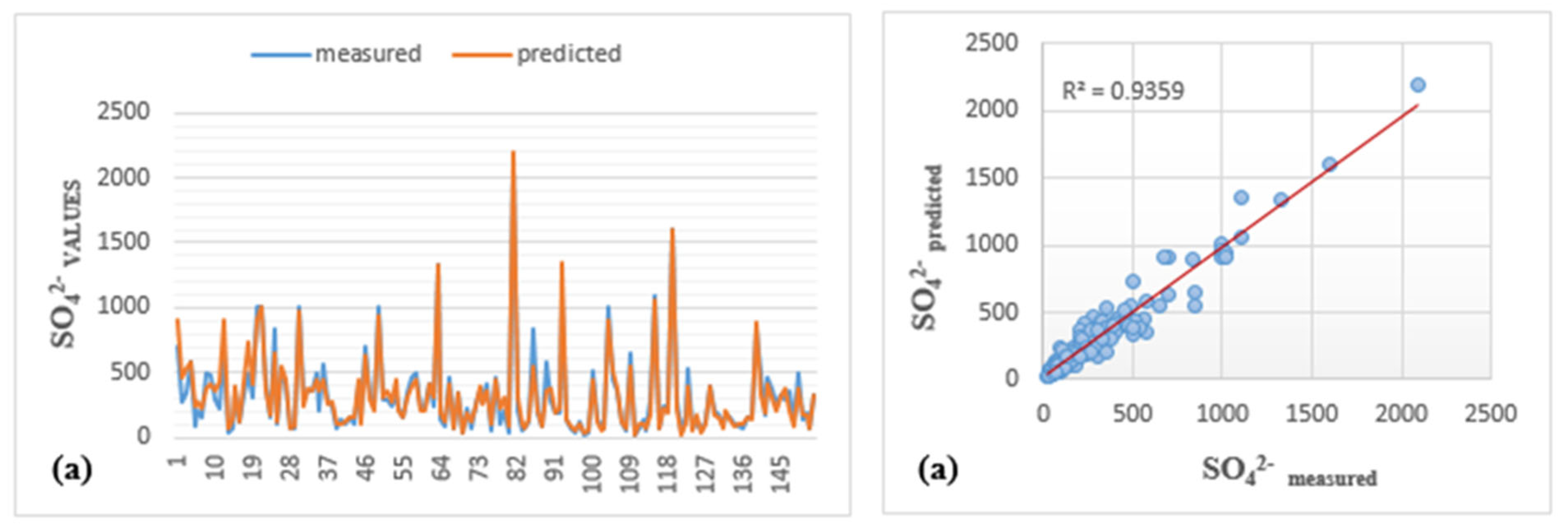
| LMBP-MLP1 | SO42− | 0.923 | 65.730 | 0.920 | 0.964 | 56.970 | 0.962 | 0.842 | 53.660 | 0.840 | 0.936 | 63.368 | 0.930 |
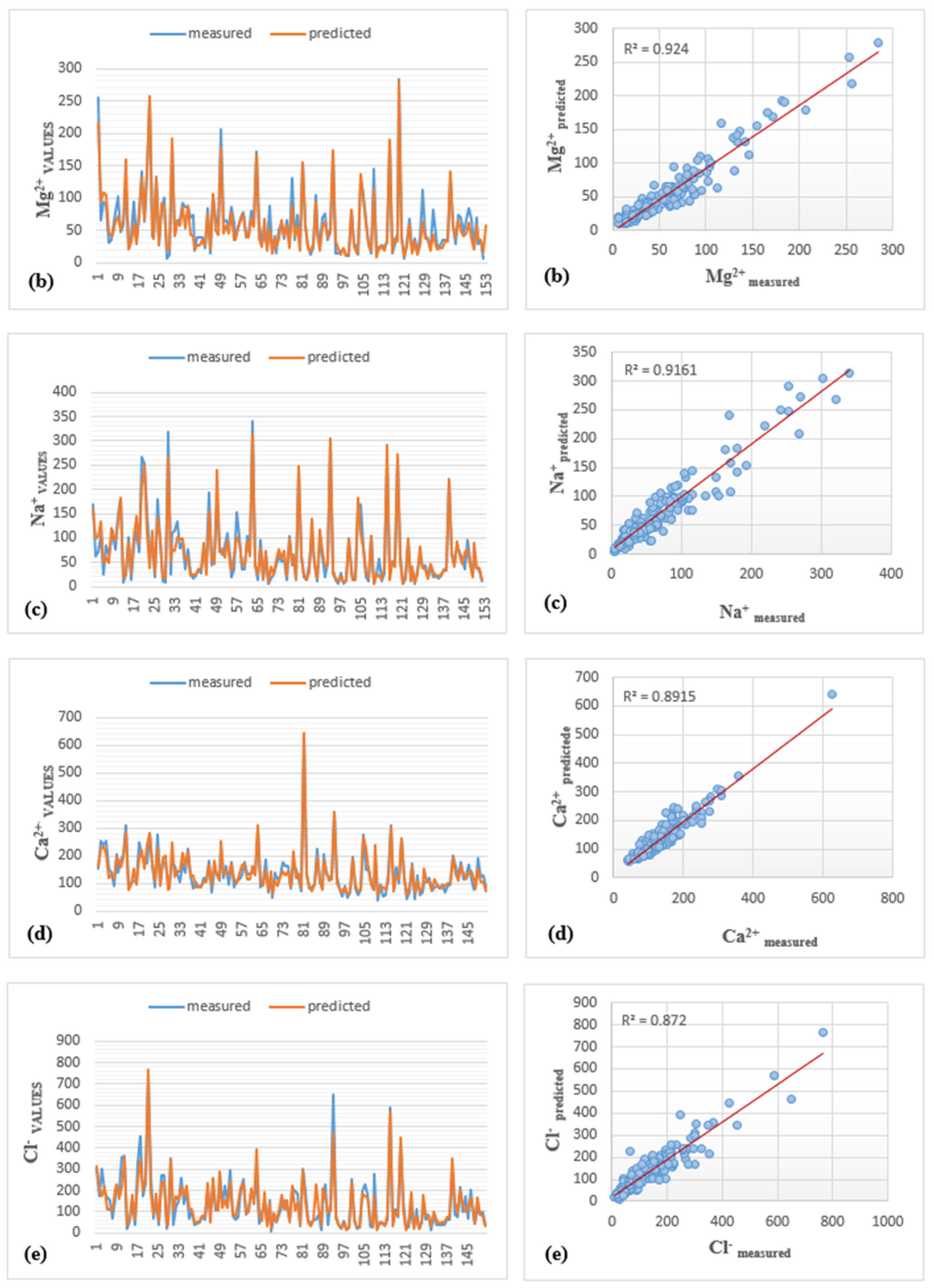
| LMBP-MLP2 | Mg2+ | 0.921 | 14.890 | 0.918 | 0.943 | 11.800 | 0.936 | 0.980 | 12.840 | 0.978 | 0.924 | 14.274 | 0.910 |
| LMBP-MLP3 | Na+ | 0.916 | 20.230 | 0.915 | 0.927 | 17.270 | 0.926 | 0.759 | 14.960 | 0.754 | 0.916 | 19.346 | 0.910 |
| LMBP-MLP4 | Ca2+ | 0.867 | 21.990 | 0.864 | 0.887 | 23.510 | 0.878 | 0.945 | 36.460 | 0.941 | 0.892 | 24.034 | 0.889 |
| LMBP-MLP5 | Cl− | 0.865 | 44.640 | 0.857 | 0.902 | 43.600 | 0.898 | 0.895 | 30.530 | 0.892 | 0.872 | 43.296 | 0.870 |
| LMBP-MLP6 | K+ | 0.533 | 2.990 | 0.535 | 0.601 | 2.850 | 0.531 | 0.045 | 6.480 | 0.003 | 0.441 | 3.482 | 0.440 |
| LMBP-MLP7 | HCO3− | 0.300 | 64.250 | 0.301 | 0.630 | 37.760 | 0.540 | 0.366 | 41.720 | 0.361 | 0.330 | 59.029 | 0.320 |
| LMBP-MLP8 | NO3− | 0.325 | 43.400 | 0.325 | 0.865 | 40.870 | 0.823 | 0.004 | 40.460 | −0.933 | 0.523 | 41.886 | 0.510 |
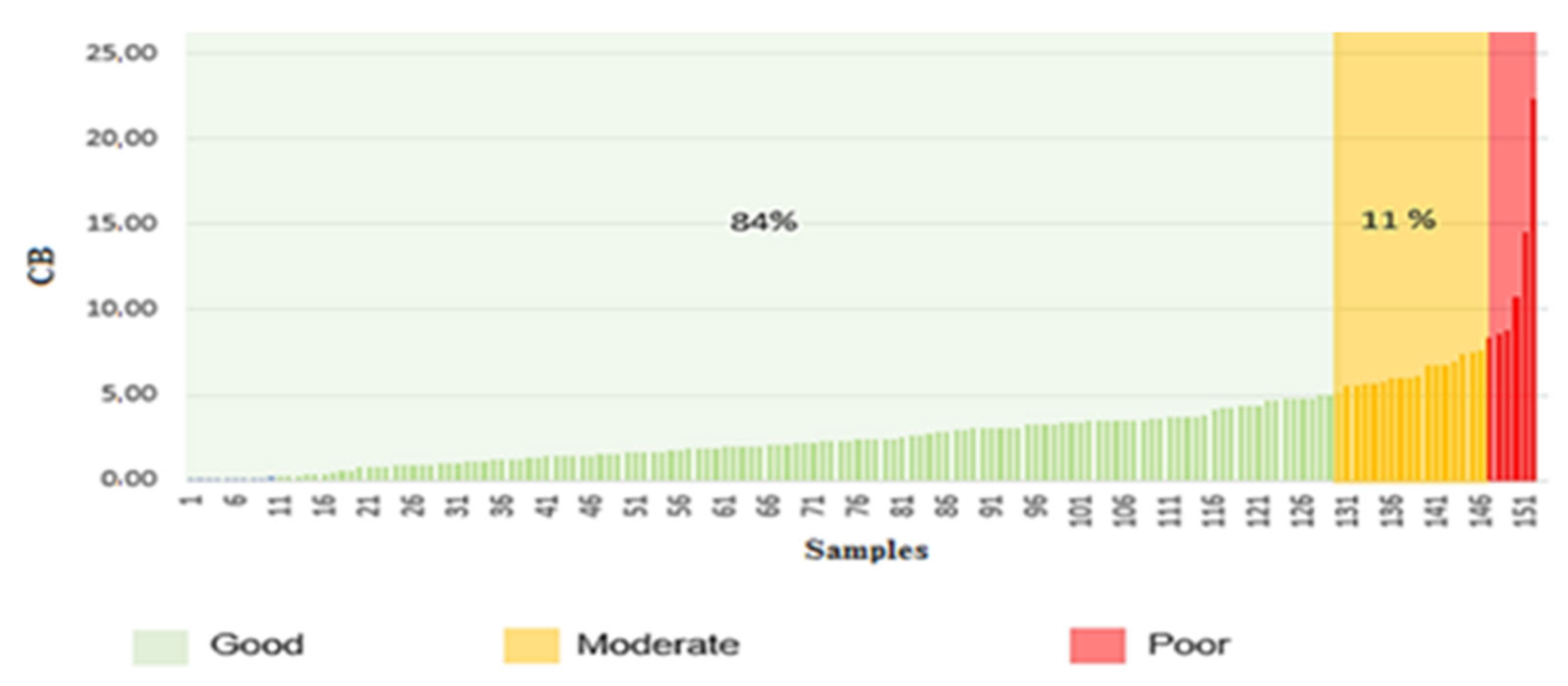
| Location | SO42− Pred. | NO3− Meas. | HCO3− Meas. | Cl− Pred. | Ca2+ Pred. | Mg2+ Pred. | Na+ Pred. | K+ Pred. | CB % | Evaluation |
|---|---|---|---|---|---|---|---|---|---|---|
| Aflou | 105 | 5 | 240 | 45 | 88 | 23 | 23 | 7 | 0.03 | Good |
| 410 | 30 | 326 | 135 | 152 | 68 | 82 | 7 | 3.54 | Good | |
| 906 | 15 | 273 | 210 | 292 | 146 | 168 | 14 | 7.45 | Moderate | |
| 393 | 14 | 239 | 190 | 153 | 61 | 86 | 7 | 3.23 | Good |
| Location | SO42− Pred. | NO3− Meas. | HCO3− Meas. | Cl− Meas. | Ca2+ Pred. | Mg2+ Pred. | Na+ Pred. | K+ Meas. | CB % | Evaluation |
|---|---|---|---|---|---|---|---|---|---|---|
| Ain Madhi | 434 | 9 | 237 | 145 | 206 | 83 | 102 | 5 | 11.60 | Poor |
| 426 | 10 | 232 | 145 | 206 | 80 | 104 | 5 | 11.90 | Poor | |
| 123 | 13 | 212 | 70 | 95 | 27 | 28 | 2 | 0.07 | Good | |
| 124 | 16 | 185 | 93 | 95 | 27 | 28 | 2 | 1.57 | Good | |
| 1677 | 4 | 237 | 400 | 177 | 298 | 270 | 15 | 4.87 | Good | |
| 1227 | 10 | 217 | 370 | 576 | 173 | 247 | 12 | 15.28 | Poor | |
| 291 | 13 | 247 | 240 | 187 | 38 | 140 | 6 | 4.51 | Good | |
| 281 | 2 | 241 | 205 | 183 | 38 | 131 | 6 | 7.40 | Moderate | |
| 352 | 5 | 162 | 220 | 163 | 50 | 104 | 15 | 2.65 | Good | |
| 257 | 34 | 144 | 155 | 128 | 41 | 58 | 6 | 0.77 | Good |
| Location | SO42− Pred. | NO3− Meas. | HCO3− Pred. | Cl− Meas. | Ca2+ Pred. | Mg2+ Pred. | Na+ Pred. | K+ Meas. | CB % | Evaluation |
|---|---|---|---|---|---|---|---|---|---|---|
| Madna | 888 | 7 | 230 | 354 | 199 | 142 | 221 | 12 | 1.28 | Good |
| 903 | 84 | 281 | 250 | 236 | 148 | 209 | 14 | 2.44 | Good | |
| 631 | 54 | 263 | 257 | 185 | 106 | 155 | 12 | 1.11 | Good | |
| 437 | 17 | 247 | 198 | 213 | 82 | 107 | 7 | 7.77 | Moderate | |
| 629 | 71 | 266 | 250 | 181 | 104 | 158 | 14 | 1.64 | Good | |
| 65 | 3 | 167 | 29 | 73 | 16 | 14 | 4 | 6.72 | Moderate |
Disclaimer/Publisher’s Note: The statements, opinions and data contained in all publications are solely those of the individual author(s) and contributor(s) and not of MDPI and/or the editor(s). MDPI and/or the editor(s) disclaim responsibility for any injury to people or property resulting from any ideas, methods, instructions or products referred to in the content. |
© 2025 by the authors. Licensee MDPI, Basel, Switzerland. This article is an open access article distributed under the terms and conditions of the Creative Commons Attribution (CC BY) license (https://creativecommons.org/licenses/by/4.0/).
Share and Cite
Stamboul, M.E.; Habib, A.; Hamimed, A.; Zakhrouf, M.; Chung, I.-M.; Kim, S. Extraction of Major Groundwater Ions from Total Dissolved Solids and Mineralization Using Artificial Neural Networks: A Case Study of the Aflou Syncline Region, Algeria. Hydrology 2025, 12, 103. https://doi.org/10.3390/hydrology12050103
Stamboul ME, Habib A, Hamimed A, Zakhrouf M, Chung I-M, Kim S. Extraction of Major Groundwater Ions from Total Dissolved Solids and Mineralization Using Artificial Neural Networks: A Case Study of the Aflou Syncline Region, Algeria. Hydrology. 2025; 12(5):103. https://doi.org/10.3390/hydrology12050103
Chicago/Turabian StyleStamboul, Mohammed Elamin, Azzaz Habib, Abderrahmane Hamimed, Mousaab Zakhrouf, Il-Moon Chung, and Sungwon Kim. 2025. "Extraction of Major Groundwater Ions from Total Dissolved Solids and Mineralization Using Artificial Neural Networks: A Case Study of the Aflou Syncline Region, Algeria" Hydrology 12, no. 5: 103. https://doi.org/10.3390/hydrology12050103
APA StyleStamboul, M. E., Habib, A., Hamimed, A., Zakhrouf, M., Chung, I.-M., & Kim, S. (2025). Extraction of Major Groundwater Ions from Total Dissolved Solids and Mineralization Using Artificial Neural Networks: A Case Study of the Aflou Syncline Region, Algeria. Hydrology, 12(5), 103. https://doi.org/10.3390/hydrology12050103