Abstract
This research presents a detailed numerical modeling study focused on estimating the concentration of microplastics (MPs) in freshwater ecosystems. This research covers three lakes (Kopa, Zerendinskoye, and Borovoe) and the Yesil River, applying differential equations to model the spatial distribution and seasonal variations in MP concentrations. The methodology integrates field survey data collected during three different seasons (spring, summer, and autumn) from both sediment and water samples. The MP concentrations were found to follow an exponential decay pattern from the shore toward the center of the lakes, with higher concentrations near the shoreline. The modeling framework is calibrated using regression analysis, which provides the best-fit parameters for the distance–concentration curves. This study employs sensitivity analysis to justify the decay coefficient, resulting in a selected value of k = 0.09. Model performance is assessed using statistical metrics such as the root mean square error (RMSE) and the coefficient of determination (R2), ensuring accuracy in predicting MP concentrations across different environmental compartments. This work represents a novel contribution to the field by applying numerical modeling techniques to an understudied geographical area. The findings highlight significant seasonal and spatial variations in MP concentrations, emphasizing the need for comprehensive monitoring. This study’s results contribute valuable insights into the environmental behavior of MPs in freshwater systems and support efforts to develop effective management strategies to mitigate pollution.
1. Introduction
1.1. Microplastic Pollution in Freshwater Systems: Sources, Risks, and Knowledge Gaps
Microplastic (MP) contamination of freshwater ecosystems has become a major environmental problem, given its pervasiveness and potential ecological impacts. MPs enter freshwater systems—rivers, lakes, and wetlands—via multiple pathways, including urban runoff, wastewater discharges, atmospheric deposition [1,2], and land-based sources such as agriculture, plastic waste mismanagement, and landfills [3,4,5], which have become hotspots for MP accumulation [6]. Despite this, freshwater systems have historically received less attention than marine environments [7], even though MP concentrations in freshwater organisms are often comparable to or higher than those found in marine species [8,9,10]. This knowledge gap is critical, given the ecological relevance of freshwater systems for biodiversity and their role as conduits transporting MPs to marine environments [11,12,13].
The ecological impacts of MP contamination in freshwater are diverse. MPs act as vectors for harmful chemicals and pathogenic microorganisms, exacerbating ecological toxicity [10,14,15,16]. They disrupt feeding behaviors and physiology in aquatic fauna [17], accumulate in food webs, and pose risks to human health through trophic transfer and drinking water contamination [3,18,19,20,21]. Nevertheless, scientific focus on lake ecosystems remains limited [9,22,23], often restricted to urban, alpine, or glacial lakes [24]. Furthermore, there is a lack of comprehensive and systematic analyses of MP sources and distribution in freshwater lakes globally [25,26]. This is concerning since lakes provide key ecosystem services (e.g., climate regulation, irrigation, and tourism) and are likely to accumulate MPs at higher rates than oceans [27].
One central challenge identified in the literature is the lack of standardized methodologies for MP sampling and analysis in freshwater environments [22,23,24,25,26,27]. The variability in sampling and detection protocols across studies significantly affects the reliability and comparability of the results [22]. This concern underscores the necessity of a consistent and rigorous data acquisition strategy, which is a strength of the present study and a prerequisite for any robust modeling approach. Spatial heterogeneity in MP distribution—driven by hydrological, climatic, and anthropogenic factors [23]—warrants spatially explicit modeling strategies. Accordingly, this study applies an exponential decay model to MP concentrations observed along lake and river transects, capturing the gradient from shoreline to central zones and reflecting the influence of shoreline use, lake morphology, and dilution.
Further reinforcing the value of sediment data in MP studies, Shi et al. [24] report substantial MP loads embedded in lakebed sediments in Tangxun Lake, China, which are not apparent from water sampling alone. This validates the decision in the current study to incorporate sediment measurements—particularly in the splash zone—as key reference points for calibrating the exponential decay model. The significance of using such empirical models is further underscored by the comprehensive review conducted by Moodley et al. [25], who classify mathematical models into empirical, statistical, and physics-based types. They highlight the practicality and adaptability of empirical models—like the one adopted here—especially in data-scarce contexts where complex hydrodynamic modeling is not feasible. This aligns with the methodological design of the present work, which leverages exponential decay relationships to approximate MP distributions based on limited but spatially and temporally representative field data.
Complementing these modeling considerations, Pan et al. [26] advocate for multi-seasonal sampling and spatially resolved analyses to better capture the dynamic nature of MP pollution in lakes. Their recommendations are directly reflected in this study’s inclusion of data from three seasons (spring, summer, and autumn) and the division of the study area into discrete spatial profiles that account for nearshore and offshore variations. Moreover, the meta-analysis by Chen et al. [27] highlights key environmental drivers, such as hydrodynamic conditions, land use, and point source pollution in determining MP concentrations. These same drivers are explicitly considered in the present modeling framework, particularly in the river segments, where successive increases and decreases in MP levels are interpreted as the combined effect of urban discharge and natural attenuation.
The methodologies used to assess MP contamination in freshwater ecosystems are critical to obtaining reliable data. Due to differences in sampling methods, stations, and detection methods, which can lead to varying results, the conclusions drawn from individual cases are not necessarily directly applicable to studies in other lakes [27]. Carvalho et al. [2] propose a standardized protocol for monitoring MP contamination, emphasizing the need for robust sample processing techniques that can effectively separate MPs from organic matter. This is especially important given the great variability in sample composition in different freshwater environments. In addition, there is a need to harmonize methods, allowing for comparable data across studies and locations, which facilitates a more complete understanding of the distribution of MPs and their ecological consequences [15,28].
Despite methodological improvements, current legislative frameworks addressing MPs in freshwater remain underdeveloped. Stronger policies are urgently needed [29]. Recent proposals by the EU Commission recommend including MPs in monitoring programs once control methods become available [30]. Hence, the development of efficient, cost-effective, and data-adapted assessment methods remains a top research and policy priority [31,32]. As D’Avignon et al. [9] note, MP concentration should be treated as an ecologically relevant water quality indicator. However, uncertainties persist regarding MP sources, accumulation rates, and temporal dynamics, which continue to hinder science-based mitigation strategies [27,33].
1.2. Microplastic Modeling Approaches and Justification of the Empirical Model Used in This Study
In recent years, the modeling of microplastics (MPs) has advanced significantly, encompassing a broad spectrum of methodologies, including hydrodynamic and process-based models, mass-balance frameworks, empirical and statistical approaches, and, more recently, machine learning techniques. These models aim to characterize the transport, fate, and accumulation of MPs in aquatic systems—both marine and freshwater—accounting for physical (e.g., advection, dispersion, and sedimentation), chemical (e.g., sorption of pollutants), and biological processes (e.g., biofouling, degradation, and ingestion by organisms) [25].
According to Moodley et al. [25], five main categories of MP modeling can be distinguished: hydrodynamic, process-based, statistical, mass-balance, and machine learning models. Each modeling framework has strengths and weaknesses depending on the environmental setting, model objectives, and data availability. Despite significant developments, the authors highlight persistent challenges across all categories, including unrealistic input assumptions, poor consideration of vertical mixing or biological processes, and lack of standardization in sampling methods. Most importantly, their review of 61 studies (2012–2022) underscores the scarcity of freshwater-focused models: only 4 in lakes and 16 in rivers, compared to 35 in marine environments—leaving important knowledge gaps in inland MP transport.
Hydrodynamic models, such as Delft3D, MIKE, TELEMAC, and ROMS, allow three-dimensional simulation of MPs, incorporating key forcings like wind, currents, tides, salinity gradients, and thermal stratification [34,35,36]. These models are valuable for detailed assessments; however, their applicability is limited by the need for high-resolution spatiotemporal input data, extensive physical forcing information, and significant computational resources—which are often unavailable in under-monitored regions such as northern Kazakhstan. Process-based models complement hydrodynamic ones by incorporating degradation, biofouling, and resuspension [37,38], although they often lack full field validation.
Statistical and mass-balance approaches have been used to estimate plastic fluxes at larger scales [39,40] but are sensitive to parameter assumptions and are less suited to describing spatially explicit behaviors. More recently, machine learning models—such as convolutional neural networks (CNNs) and support vector machines (SVMs)—have emerged for pattern recognition and rapid classification of microplastics in laboratory and field samples [41,42], though their use in predicting transport and fate is still incipient.
In data-scarce environments, empirical models—particularly those based on exponential or logarithmic decay functions—offer a viable and practical alternative. These models have been effectively used in marine and lacustrine environments to characterize spatial MP concentration gradients arising from dilution, deposition, and reduced inputs away from anthropogenic sources [26,27]. They are particularly suitable for identifying first-order spatial trends when process-level understanding or hydrodynamic calibration data are lacking.
This study adopts a first-order exponential decay model to represent the spatial distribution of MPs across lake transects and river profiles. This approach is supported by consistent empirical observations showing a systematic decrease in MP concentrations from the splash zone toward open water—a pattern reported in similar lacustrine systems [24,27]. This gradient likely results from physical processes such as dilution, settling, and a decrease in direct source contributions with increasing distance from shorelines. The results presented in this work were obtained from a comprehensive sampling campaign assessing MP content in three lakes and one river in northern Kazakhstan. To the best of the authors’ knowledge, this is the first numerical modeling study on MP concentrations in rivers and lakes conducted in this region of Central Asia.
Moodley et al. [25] emphasize that empirical models are especially useful for baseline assessments in developing countries or remote areas, where detailed hydrodynamic modeling is not feasible. When calibrated with field data—as performed in this study—such models can robustly capture the spatial dynamics of MPs. Moreover, they offer simplicity, transparency, and ease of calibration, all of which are critical when integrating results into environmental policy or local monitoring programs. The empirical, spatially calibrated exponential decay models applied to both lake and river data in this study align with global best practices for MP modeling while addressing the specific challenges of an underrepresented geographic region.
Although the empirical model applied here does not explicitly simulate vertical dynamics or interactions with biological processes, it provides a reproducible and spatially explicit first approximation of MP behavior. This type of model can serve as a starting point for future developments incorporating coupled or hybrid modeling strategies, including machine learning, Bayesian inference, or integration with hydrodynamic models [8]. By incorporating both sediment and water data, accounting for seasonal variability, and applying sensitivity analyses to calibrate model parameters, this study contributes a structured and reproducible methodology that can serve as a reference for similar assessments in other freshwater systems worldwide.
2. Materials and Methods
2.1. Description of the Study Area and Previous Works
The study area comprises the Yesil River and three major lakes—Kopa, Zerendinskoye, and Borovoe—located in the Akmola Region of northern Kazakhstan (Figure 1). These water bodies were selected due to their ecological and socio-economic importance, high anthropogenic pressure, and observed or potential microplastic (MP) pollution. Their geographical settings, hydromorphological features, and human influences are particularly relevant for constructing and calibrating hydrodynamic and transport models aimed at simulating MP distribution and behavior.
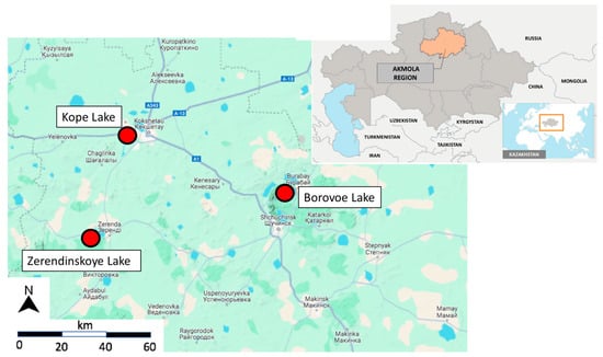
Figure 1.
Location of Kopa, Zerendinskoye, and Borovoe lakes, as originally included in [43].
The lakes selected for monitoring are typical shallow water bodies with recreational and ecological significance, subject to urban, peri-urban, and tourism-related pressures. Lake Kopa is located in the city of Kokshetau and has a surface area of 14 km2, with depths ranging from 2 to 3 m. It is fed by the Chaglinka and Kylshakty rivers and characterized by soft sediment layers, dense aquatic vegetation, and multiple pollution sources, including wastewater discharges and runoff from railway infrastructure.
Lake Borovoe, situated at the base of Mount Kokshe, is a closed-basin lake with an area of 10.5 km2 and average depths between 4.5 and 7 m. It is a major tourist attraction, particularly during summer, with various anthropogenic structures near the shore. This makes it susceptible to MP pollution from recreational activities and infrastructure, providing a context to study spatial gradients and accumulation mechanisms.
Lake Zerendinskoye, with an area of 9.6 km2, is located approximately 50 km from Kokshetau. It has fresh, transparent water, flat sandy bottoms, and limited tourist influence compared to Borovoe, though several facilities, such as schools, health centers, and fishery operations, are present along its shoreline.
The Yesil River is the primary fluvial system in the Akmola Region. It flows from the southeast to the northwest, eventually entering the North Kazakhstan region [44]. The regional segment under study spans approximately 1027 km, draining an area of around 20,000 km2. It features marked seasonality in hydrological regimes, with stable ice cover forming by late November and spring floods peaking between May and June. The influence of summer precipitation on discharge is minimal. Within the urban setting of Astana, the Yesil River is subjected to diverse point and diffuse pollution sources, including industrial zones, overflow dams, recreational embankments, and tributaries such as the Akbulak River. These conditions provide a heterogeneous context for MP input, making the river a dynamic environment for modeling pollutant fate and transport.
This study included extensive and systematic sampling of both water and sediments across seasons (spring, summer, and autumn of 2023). A total of 64 water samples were collected at different depths (surface and 1.5 m) and locations within each water body. Water sampling was conducted using standard volumetric techniques, with filtration through 100 µm mesh to extract MPs. Each sampling campaign considered the hydrodynamic regime, accessibility, and potential pollution sources. Sediment sampling was equally thorough, with 30 designated sites classified into three key zones: open water bottom sediments, water’s edge, and splash zone. This zoning allowed for the assessment of spatial variability and sediment–water interactions regarding MP accumulation. In addition, beach sediments were sampled perpendicularly to shoreline profiles to understand depositional dynamics under wind and wave action.
These sampling activities and the detailed spatial coverage provide critical boundary and calibration data for numerical models aimed at simulating microplastic transport. The model can be informed by flow regime data, sediment characteristics, and observed concentration patterns across various environmental compartments. This level of detail ensures robustness in evaluating MP behavior, identifying hotspots, and projecting the impact of management scenarios in both fluvial and lacustrine environments.
Detailed information about the sampling methodology and data acquisition can be found in a previous work by the authors [43], which details the location of the water bodies (lakes and river), the location of the sampling points, the dates of sampling, and the laboratory results. The microplastic concentration data in the river and the lakes are taken from this previous publication as input data used to calibrate the exponential decay model shown in the next sections.
2.2. Numerical Modeling of Environmental Processes Using Differential Equations
Environmental science is critically important when addressing global issues such as ecosystem conservation, sustainable development, and human well-being [45]. In this field, differential equations play a key role by allowing scientists to describe the complex dynamics of environmental systems through mathematical models [46,47]. The use of differential equations enables a deeper analysis of environmental problems and helps to devise effective solutions [48,49]. As a result, differential equations are an essential tool in environmental science modeling, providing scientists with a clearer understanding of environmental systems and a scientific foundation for tackling environmental challenges.
In environmental science, differential equation modeling follows clear steps [47]. First, the problem is defined, the relevant theory is applied, data are collected, and then the hypothesis is established. For example, suppose that pollutants are evenly distributed in a body of water. Second, formulaic models of differential equations that describe, for example, changes in pollutant concentrations over time and space are used to solve these equations with the aim of obtaining analytical or numerical solutions. Finally, after verification and adjustment with experimental data, the model is used for forecasting and actual environmental management decisions.
For example, consider the diffusion and degradation of pollutants, which can be described using the first-order differential equation shown in Equation (1):
where C is the concentration of the pollutant, and k is a normal number representing the degradation rate.
By separating and integrating the variables, Equation (2) is obtained, showing that the concentration decreases exponentially with time, where Co is the initial pollutant concentration.
Eberhardt et al. [50] suggest that the solutions of these differential equations do not fit the field data well. The main difficulty seems to be that some of the coefficients of the K-matrix are not constants but change in time, often relatively rapidly. Therefore, one must replace such coefficients with functions of time, complicating the model considerably and often leading to intractable equations. Models with constant coefficients can, however, be quite useful in appraising laboratory studies and short-term field studies.
Although simplified, this model provides a basis for practical applications and can be extended as needed, such as to account for spatial distribution and changes in environmental conditions.
2.3. Numerical Modeling of the Concentration of MPs in Lakes
2.3.1. Description of Sampling Data Locations in Lakes
The numerical modeling approach proposed in this study is based on the results of a field survey campaign [43], which allowed for the determination of MP concentrations in sediment and water samples collected from the following points in the lakes:
- Three sediment samples taken from the shoreline of the lake.
- Two freshwater samples collected near the coast and within the interior of the lake.
The sediment samples are located in the splash zone (point ZZ), at the water’s edge (point SW), and in the bottom sediments (point DO), which are separated by 0.85 m and 7.5 m, respectively. The water samples were taken 20 m and 1500 m from the shore, at a depth of 1.5 m.
Figure 2 provides a schematic representation of the location of these sampling points inside each one of the cross-sectional profiles of the lakes. Points A and B in Figure 2 represent the locations where two freshwater samples were collected—one near the coast and the other within the interior of the lakes. These points were selected to analyze the variation in microplastic concentrations between nearshore and offshore water samples.
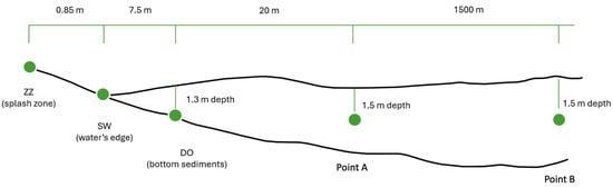
Figure 2.
Location of the sampling points inside the cross-sectional profiles of the lakes.
The GPS coordinates of all the sampling points were recorded [43]. Three different sampling campaigns were conducted, corresponding to the three seasons: spring, summer, and autumn.
2.3.2. Description of the Conceptual Model
For each of the cross-sectional profiles where information is available, a variation model of MP concentration has been fitted. To do this, it was first verified that the highest concentrations were observed in sediment samples from the splash zone (ZZ) and that these concentrations decrease as we approach the center of the lake.
Regression analysis was carried out in order to establish the relation between the independent variable and the dependent variable lo. In this context, it can be used to find the correlation between the MP concentration and the distance in the lake. After this, optimization techniques are used to obtain the best fit parameters for distance–MP concentration characteristic curves, which follow an exponential decay. In order to further sharpen the model so developed, statistical tools can be used to analyze the model behavior to check whether the system is free from error and accuracy of the system in terms of error performance can be verified. For accessing the quality of the proposed model, accurately studying the prediction error is of utmost importance.
However, some techniques available may create misleading results, which might lead to over-fitting the data. The concept behind over-fitting comes into the picture when the training data are fitted very well, but the model fails when new datasets are used as test data. The main aim should be to build up a model that predicts well for new datasets used for testing. Preventing over-fitting and under-fitting is the key to building up robust and reliable systems [51].
In this work, the root mean square error (RMSE) and the coefficient of determination (R2) were used to study the system performance. The RMSE and R2 are two key statistical parameters for evaluating the performance of predictive models, particularly in engineering and environmental science contexts. These metrics provide information on the accuracy and reliability of models that simulate environmental processes, such as pollution prediction, water quality assessment, and ecological modeling.
The RMSE (Equation (3)) is a measure of the differences between predicted and observed values, which quantifies the model’s prediction error.
where = observed experimental data; = predicted data; and N = number of observations.
A lower RMSE indicates a better fit of the model to the data, as it reflects smaller discrepancies between predicted results and actual measurements. It is especially useful because it gives more weight to larger errors, making it sensitive to outliers.
On the other hand, the R2 (Equation (4)) provides a measure of how well the independent variables explain the variability of the dependent variable. A value of R2 close to 1 indicates a better fit of the model to the data.
where SSE = residual sum of squares = ; SST = total sum of squares = ; and = average of the data.
In the study and modeling of MPs, these two metrics have been calculated to validate the models used. Huda et al. [52,53] compared polynomial regression and machine learning models for predicting MP concentrations in beach sediments using the RMSE. In a review of methods for modeling MP transport in marine environments, the R2 was highlighted as a crucial metric for validating the robustness of various modeling approaches, including hydrodynamic and statistical models [34].
In environmental engineering, the R2 is often presented together with the RMSE to provide an overall view of model performance. In Agboola and Benson’s study [54], the authors examined the interactions of MPs with organic chemical contaminants, employing both the RMSE and R2 to evaluate their predictive models. This dual approach allows not only quantifying prediction errors but also understanding the proportion of variance explained by their models, leading to more informed conclusions about the environmental implications of their findings. In the context of freshwater ecosystems, models that predict the transport and fate of MPs can be evaluated using the RMSE and R2 to ensure that they accurately reflect real-world conditions. This is especially relevant in studies assessing the impact of land use on MP concentrations in river waters, as demonstrated by Zhang [55], who provided insights into the characteristics and distribution of MPs while emphasizing the importance of robust modeling techniques.
Therefore, the calibration of the parameters characterizing the exponential model was performed as follows:
- Co: Concentration observed in the sediments of the splash zone (ZZ) in each cross-sectional profile;
- k: Coefficient to be calibrated for the three lakes analyzed in northern Kazakhstan.
The calibration of the exponential coefficient k, which ultimately characterizes the geometry of the concentration curve, must be justified through a sensitivity analysis, comparing the adjustments made in each of the cross-sectional sections studied.
As it is explained in Section 3, in the case of the three lakes studied, all located in northern Kazakhstan, the final value chosen, which provides the best overall fit, was k = 0.09.
For future modeling efforts at other locations or those incorporating a greater amount of data, this value must be verified.
2.4. Numerical Modeling of the Concentration of MPs in Yesil River
2.4.1. Description of Available Data
The numerical modeling approach proposed in this study is based on the results of a field survey campaign, which allowed for the determination of MP concentrations in water samples collected from different sampling points located in the river:
- Samples taken at the water surface;
- Samples taken at 1.5 m below the water surface.
Figure 3 shows the location of the sampling points in the Yesil River. The GPS coordinates of all the sampling points were recorded [43]. For this set of samples, MP concentrations were measured. Water is flowing from sampling point 6 to sampling point 1, defining a one-dimensional profile for which the microplastic concentration is to be modeled. Three different sampling campaigns were conducted, corresponding to the three seasons where the water is not covered by ice: spring, summer, and autumn.
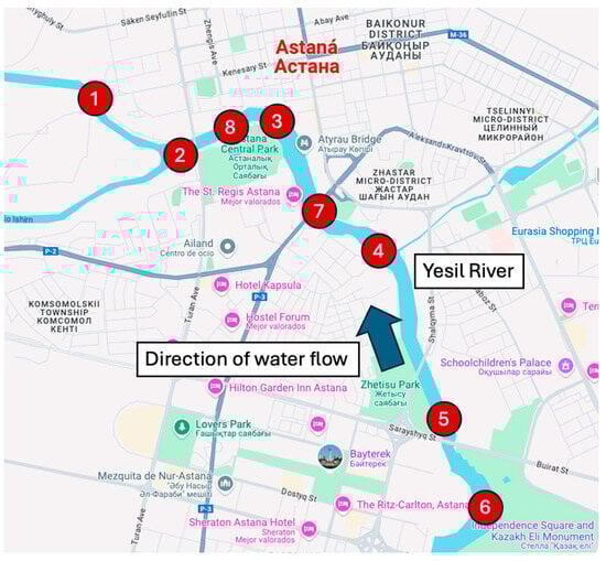
Figure 3.
Location of sampling points in the Yesil River (as originally included in [43]) and direction of the water flow.
2.4.2. Description of the Conceptual Model
The evolution of MP concentration along the river course can be described by concatenating exponential models of the type . To perform this process, the following process is necessary for each dataset corresponding to each station (Figure 4):
- Plot the MP concentration data along the river course.
- Identify river sections where the concentration is decreasing.
- Identify sections where wastewater discharge occurs, causing an increase in MP concentration.
- Perform a parameter sensitivity analysis to determine the optimal value of the exponential decay coefficient (k).
- Perform an independent calibration to calibrate the value of the maximum initial concentration at each discharge point (C0-i), whose positions should have been previously established.
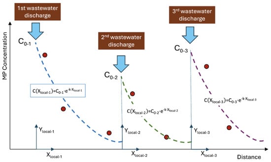
Figure 4.
Conceptual model of the evolution of the concentration of MP along the river course.
The values of the exponential decay coefficient may vary from season to season but must remain constant for all exponential models fitted along the river course for a given season.
As shown in Figure 4, once the value of k is established, it remains to determine the exact position of the discharge points and the corresponding maximum concentration values. In the absence of more information, the position of the discharge points can be determined at the midpoint between two measurement points between which the concentration increases.
The value of the maximum initial concentration in each section must be determined from the corresponding fit. To do this, the criterion of minimizing the root mean square error (RMSE) or maximizing the coefficient of determination (R2) can be used, as was proposed for the case of modeling MP concentration in lakes.
3. Results and Discussion
3.1. Kopa Lake
Figure 5 shows the location of the sampling points in Kopa Lake. In this lake, water samples were taken at a depth of 1.5 m at points 1 to 8, and sediment samples were collected at three locations near points 2 and 6, with the aim of analyzing the concentration of MPs. To study the correlation in MP concentration, profiles 2-8 and 6-8 were analyzed.
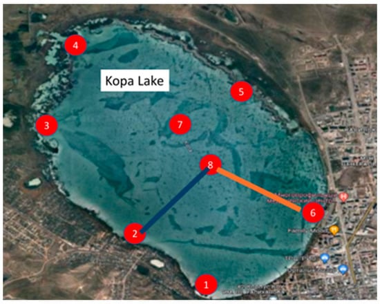
Figure 5.
Location of sampling points and cross-sections in Kopa Lake.
Water samples were collected on three different dates (spring, summer, and autumn) to measure MP concentrations. Only one sediment sample is available for each of the two analyzed sections (2-8 and 6-8). For this reason and modeling purposes, the average annual concentration of MPs in sediments was calculated. The average concentration is used because the exact dates of the sediment sample collection are not available, and only one sediment sample is available for each of the analyzed sections. All these analysis results are shown in Table 1.

Table 1.
Concentration of MPs in water and sediment samples. Kopa Lake.
Therefore, the coefficients of the calibrated model and the values of the R2 and RMSE for profiles 2-8 and 6-8 are shown in Table 2.
Table 2.
Coefficients of the calibrated model for Kopa Lake profiles.
Equations of the calibrated model for Kopa Lake profiles are shown in Equation (5) (profile 2-8) and Equation (6) (profile 6-8):
The MP concentration vs. distance graph for the profiles 2-8 and 6-8 are shown in Figure 6.
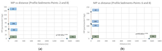
Figure 6.
MP concentration vs. distance for Kopa Lake profiles: (a) profile 2-8; (b) profile 6-8.
The MP concentration vs. distance graph for the first 30 m from the shore on the profiles is shown in Figure 7.
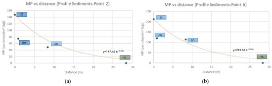
Figure 7.
MP concentration vs. distance for the first 30 m from the shore on Kopa Lake profiles: (a) profile 2-8; (b) profile 6-8.
3.2. Zerendinskoye Lake
Figure 8 shows the location of the sampling points in Zerendinskoye Lake. In this lake, water samples were taken at a depth of 1.5 m at points 1 to 8, and sediment samples were collected at three locations near points 1, 5, and 6, with the aim of analyzing the concentration of MPs. To study the correlation in MP concentration, profiles 1-8, 5-7, and 6-7 were analyzed.
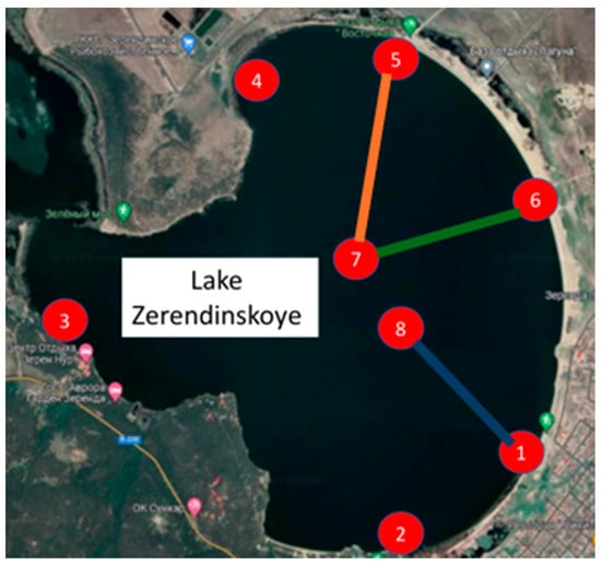
Figure 8.
Location of sampling points and cross-sections in Zerendinskoye Lake.
For this lake, the sampling strategy followed the same approach as described for Kopa Lake. The results are shown in Table 3.
Table 3.
Concentration of MPs in water and sediment samples. Zerendinskoye Lake.
Therefore, the coefficients of the calibrated model and the values of the R2 and RMSE for profiles 1-8, 5-7, and 6-7 are shown in Table 4.
Table 4.
Coefficients of the calibrated model for Zerendinskoye Lake profiles.
Equations of the calibrated model for Zerendinskoye Lake profiles are shown in Equation (7) (profile 1-8), Equation (8) (profile 5-7), and Equation (9) (profile 6-7):
The MP concentration vs. distance graph for whole profiles is shown in Figure 9.
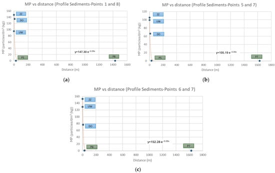
Figure 9.
MP concentration vs. distance for Zerendinskoye Lake profiles: (a) profile 1-8; (b) profile 5-7; (c) profile 6-7.
The MP concentration vs. distance graph for the first 30 m from the shore on the profiles is shown in Figure 10.
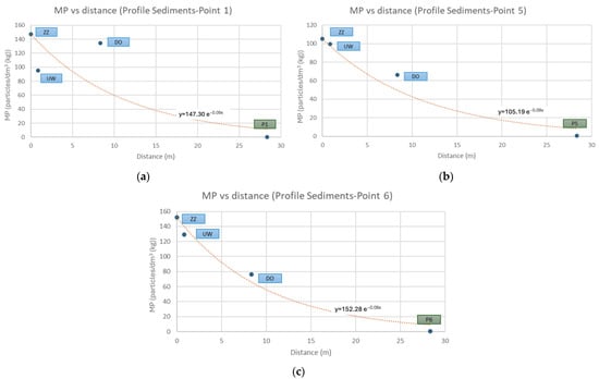
Figure 10.
MP concentration vs. distance for the first 30 m from the shore on Zerendinskoye Lake profiles: (a) profile 1-8; (b) profile 5-7; (c) profile 6-7.
3.3. Borovoe Lake
Figure 11 shows the location of the sampling points in Borovoe Lake. In this lake, water samples were taken at a depth of 1.5 m at points 1 to 8, and sediment samples were collected at three locations near points 4, 5, and 6, with the aim of analyzing the concentration of MPs. To study the correlation in MP concentration, profiles 4-8, 5-8, and 6-8 were analyzed.
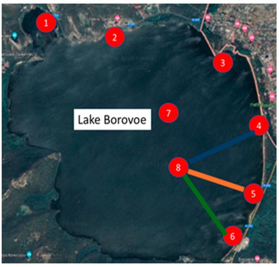
Figure 11.
Location of sampling points and cross-sections in Borovoe Lake.
As in the two previous lakes, the sampling strategy followed the same approach. The results are shown in Table 5.
Table 5.
Concentration of MPs in water and sediment samples. Borovoe Lake.
Therefore, the coefficients of the calibrated model and the values of the R2 and RMSE for Borovoe Lake profiles are shown in Table 6.
Table 6.
Coefficients of the calibrated model for Borovoe Lake profiles.
The calibrated model equations for Borovoe Lake profiles are provided in Equation (10) (profile 4-8), Equation (11) (profile 5-8), and Equation (12) (profile 6-8):
The MP concentration vs. distance graph for whole profiles is shown in Figure 12.
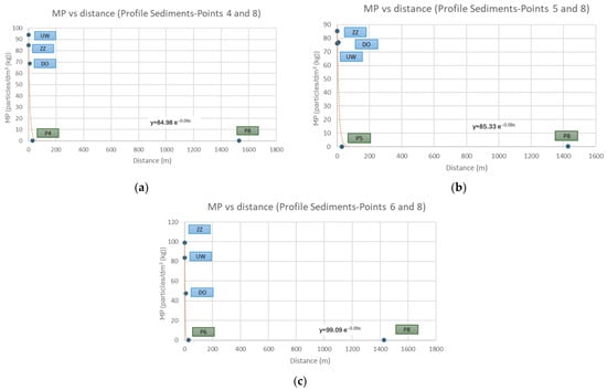
Figure 12.
MP concentration vs. distance for Borovoe Lake profiles: (a) profile 4-8; (b) profile 5-8; (c) profile 6-8.
The MP concentration vs. distance graph for the first 30 m from the shore on the profiles is shown in Figure 13.
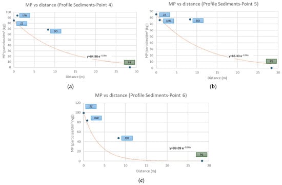
Figure 13.
MP concentration vs. distance for the first 30 m from the shore on Borovoe Lake profiles: (a) profile 4-8; (b) profile 5-8; (c) profile 6-8.
3.4. Yesil River
In the river, water samples were collected on three different dates (spring, summer, and autumn). The results of these analyses are shown in Table 7.
Table 7.
Concentration of MPs in water samples. Yesil River.
A visual representation of the variability of the concentrations of microplastics on the profile is shown in Figure 14 (water surface data) and Figure 15 (1.5 m depth data). In many cases, and for all the seasons, MP concentrations at 1.5 m depth are higher than those found at the water surface.
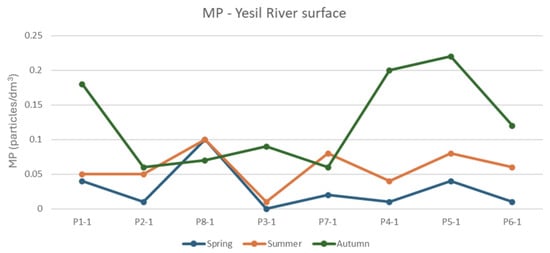
Figure 14.
MP concentrations at water surface for the three seasons.
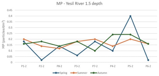
Figure 15.
MP concentrations at 1.5 m depth for the three seasons.
For modeling purposes, the MP concentrations data have been obtained as the average of the available data at the water surface and at 1.5 m depth.
3.4.1. Modeling of Autumn Data
Figure 16 shows the average MP concentration values in autumn, obtained as the average of the available data measured at the water surface and those measured at 1.5 m depth. Figure 16 shows that two profiles should be modeled: profile 4-7 and profile 3-8. Following the conceptual model explained in Section 2.4.2, each one of these profiles should be modeled independently.
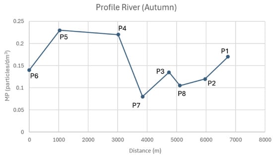
Figure 16.
Average MP concentration values in autumn.
Figure 17 shows the adjusted model for river profiles in autumn. The values of the coefficients (C0 and k) for the calibrated model, considering the values obtained for a set of simulations, are shown in Table 8.
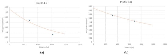
Figure 17.
Adjusted model for river profiles in autumn: (a) profile 4-7; (b) profile 3-8.
Table 8.
Coefficients of the calibrated model in autumn. Yesil River.
Therefore, the equations of the calibrated model for Yesil River profiles in autumn are shown in Equation (13) (profile 4-7) and Equation (14) (profile 3-8):
3.4.2. Modeling of Summer Data
Figure 18 shows the average MP concentration values in autumn, obtained in the same way as in the autumn period. Figure 18 shows that four profiles should be modeled independently: profile 6-5, profile 4-7, profile 3-8, and profile 2-1.
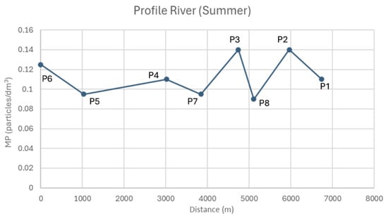
Figure 18.
Average MP concentration values in summer.
Figure 19 shows the adjusted model for river profiles in summer. The values of the coefficients (C0 and k) for the calibrated model, considering the values obtained for a set of simulations, are shown in Table 9.
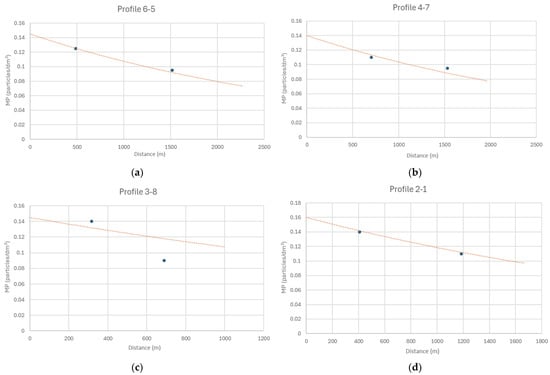
Figure 19.
Adjusted model for river profiles in summer: (a) profile 6-5; (b) profile 4-7; (c) profile 3-8; (d) profile 2-1.
Table 9.
Coefficients of the calibrated model in summer. Yesil River.
Therefore, the equations of the calibrated model for Yesil River profiles in summer are shown in Equation (15) (profile 6-7), Equation (16) (profile 4-7), Equation (17) (profile 3-8), and Equation (18) (profile 2-1):
3.4.3. Modeling of Spring Data
Figure 20 shows the average MP concentration values in spring, which were obtained in the same way as in the other periods. Figure 20 shows that the profiles to be modeled are the same as in the summer period.
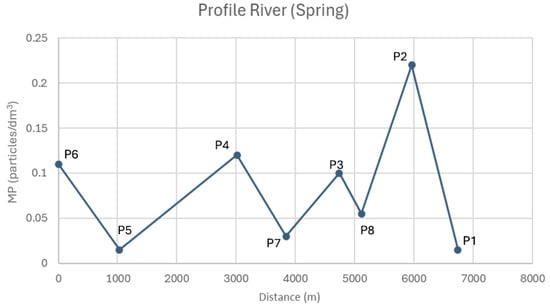
Figure 20.
Average MP concentration values in spring.
Figure 21 shows the adjusted model for river profiles in spring. The values of the coefficients (C0 and k) for the calibrated model, considering the values obtained for a set of simulations, are shown in Table 10.
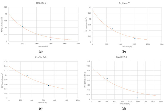
Figure 21.
Adjusted model for river profiles in spring: (a) profile 6-5; (b) profile 4-7; (c) profile 3-8; (d) profile 2-1.
Table 10.
Coefficients of the calibrated model in spring. Yesil River.
Therefore, the equations of the calibrated model for Yesil River profiles in spring are shown in Equation (19) (profile 6-7), Equation (20) (profile 4-7), Equation (21) (profile 3-8), and Equation (22) (profile 2-1):
The justification of the exponential decay parameter value (k) in the lakes and the maximum initial concentration (C0) and the exponential decay parameter value (k) in the river is contained in the Supplementary Material, in Tables S1–S13.
Accounting for the results obtained, Figure 22, Figure 23 and Figure 24 show the modeling profiles of the Yesil River in autumn, summer, and spring, respectively.
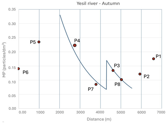
Figure 22.
Adjusted model for autumn. Yesil River.
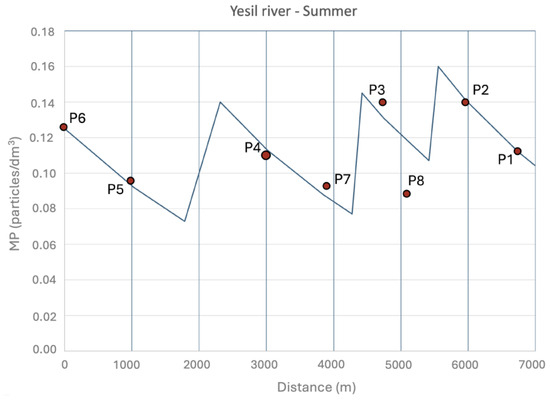
Figure 23.
Adjusted model for summer. Yesil River.
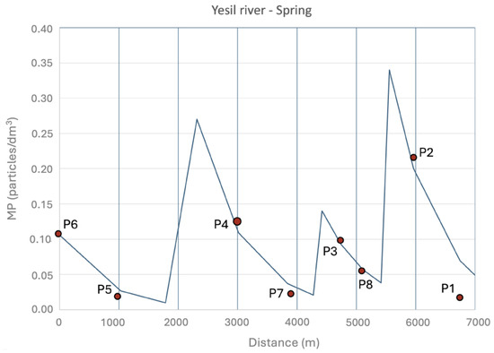
Figure 24.
Adjusted model for spring. Yesil River.
The results shown in the figures are satisfactory, even accounting for the extremely linted amount of data. The observed data are adequately reproduced by the model, particularly during the summer and spring seasons. However, the model struggles to reproduce the autumn data corresponding to sampling points P6, P5, P2, and P1, as increasing MP concentrations are observed at these points.
The variation in k values for the river across different seasons is likely influenced by seasonal hydraulic conditions. During periods of higher flow, such as spring and early summer, increased discharge and turbulence can enhance MP resuspension, transport, and dilution, leading to a slower decay of concentration along the river profile (i.e., lower k values). Conversely, in lower flow conditions, reduced turbulence and sedimentation processes may cause MPs to settle more quickly, resulting in steeper concentration gradients and higher k values. This explanation aligns with studies on MP transport in rivers, where hydrodynamic forces strongly influence the dispersion and retention of particles in different flow regimes.
The sources identified through modeling can be linked to site-specific activities. The model indicated localized increases in MP concentrations at certain points along the Yesil River, suggesting possible inputs from urban wastewater discharges, stormwater runoff, or industrial effluents. These results highlight the need to integrate hydrodynamic data and land use assessments in future research to refine PM transport models. The seasonal dependence of k values underscores the importance of accounting for dynamic flow conditions when assessing the fate of PM in freshwater systems. In future work, field-measured flow velocity, discharge rates, and sediment transport parameters could be incorporated to strengthen the predictive capabilities of the model considered in this research, which reproduces the concentration of microplastics in rivers and lakes in the Akmola area.
4. Limitations and Further Research
In the absence of prior studies addressing the decay of microplastic (MP) concentrations in freshwater ecosystems of the Akmola Region, this study represents a preliminary effort to model MP concentration trends in lakes and rivers using an exponential decay approach.
The choice of a first-order exponential decay model for the spatial variation in microplastic (MP) concentrations was based on both theoretical considerations and empirical evidence from field measurements. This approach aligns with well-established contaminant transport models used in environmental engineering, as indicated in the manuscript with bibliographic references. The field measurements indicated that MP concentrations were highest at the shoreline and decreased progressively toward open water, following an exponential trend. Regression analysis confirmed that the decay pattern of MP concentrations with distance from the shore closely matched an exponential function, supporting the suitability of a first-order model. Therefore, in view of the results obtained, the model used provides a first valid fit that explains the concentration of PM in these freshwater ecosystems.
The model was formulated for cross-sectional profiles, analyzing transport perpendicular to the shoreline, where gradual dilution and sedimentation dominate. The assumption of unidirectional transport is reasonable at the local scale of each profile because wind-driven currents and density stratification primarily disperse MPs offshore. Moreover, lateral mixing and long-term recirculation occur at larger scales. Based on the results obtained in this modeling, possible future research would be to incorporate hydrodynamic models to capture these effects in a more explicit and local way.
To improve the understanding of MP pollution dynamics, future research should incorporate seasonally adjusted monitoring strategies that account for peak contamination periods and potential resuspension events. The integration of hydrodynamic and sediment transport measurements into these monitoring programs will enable a more comprehensive characterization of MP behavior. Although the current study provides a first-order approximation of MP distribution in the region’s freshwater bodies, future model refinements should include key hydrodynamic parameters such as flow velocity, turbulence, and sediment interactions to enhance predictive capability and accuracy.
The modeling framework developed herein is adaptable to other freshwater systems with diverse hydrological and geographical characteristics, including larger river networks and reservoirs, thereby facilitating assessments of how land use, wastewater discharges, and urbanization influence MP pollution. Technological advancements, such as remote sensing, microplastic tracking techniques, and artificial intelligence-based modeling, present promising opportunities to improve MP detection, distribution analysis, and fate prediction. As more studies on MP modeling in freshwater environments and across varying geographical contexts become available, comparative assessments will become increasingly feasible. To support this advancement, future research should aim to expand the dataset through additional sampling campaigns in both lakes and rivers and integrate outputs from hydrodynamic and sediment transport models to further validate and enhance the robustness of the proposed modeling approach.
5. Conclusions
This report presents a modeling methodology for determining MP concentrations in lakes and rivers based on a limited dataset obtained from a field survey campaign. For both lakes and rivers, the proposed methodology is grounded in the determination of the parameters (k and C0) characterizing a decreasing exponential model, expressed as . This model is widely used in environmental engineering to describe the spatial variation in contaminant concentrations.
For lakes, the proposed model has been applied to data from sampling campaigns conducted in Lakes Kopa, Zerendinskoye, and Borovoe, located in North Kazakhstan. The modeling results demonstrate satisfactory fits, even with an extremely limited dataset. A sensitivity analysis has led to the adjustment of a single decay coefficient (k = 0.09) for the exponential model, common to all three lakes. A total of eight transverse profiles, extending from the shores to the lake centers, were analyzed. The maximum concentration value in each profile (C0) corresponds to the MP concentration in the sediments at the point farthest from the lake center. Thus, the proposed model enables the determination of concentrations in sediments or water at any point in the lake, simply by determining the pair of values C0 and k.
For rivers, the proposed model has been applied to data from a sampling campaign conducted on the Yesil River as it passes through Astana. In this case, MP concentration values were available at only eight points along the river’s longitudinal profile. Consequently, a one-dimensional transport model was proposed. Given the variable MP concentrations along the river, with observed increases and decreases, it was necessary to calibrate successive models defined for each river section. This variability may be attributed to the presence of point sources along the river, whose positions were clearly identified in the different sections.
The sensitivity analysis for the exponential model of microplastic (MP) concentration showed that a single decay coefficient (k) was sufficient for lakes, but in the Yesil River, seasonal variations allowed for the calibration of distinct k values for spring, summer, and autumn. The seasonal variation in k is mainly attributed to hydrodynamic conditions: high flows during spring and early summer lead to lower k values due to enhanced MP transport and dilution, while lower flows in other seasons increase k values due to greater sedimentation and retention. The model also revealed that MP sources in the Yesil River are linked to localized human activities such as urban wastewater, stormwater, and industrial discharges, while in lakes, higher concentrations near shores are likely due to recreational activities, runoff, and organic debris accumulation.
The results indicate that MP transport and distribution are dependent on seasonal hydrodynamic conditions, with differences in decay coefficients (k values) suggesting that flow rates, turbulence, and sedimentation dynamics influence MP retention and dispersion in both lakes and rivers. These seasonal differences should be considered when designing remediation approaches. For instance, during high-flow periods (spring and early summer), MPs are likely to remain suspended for longer distances due to increased turbulence and flow velocity. In contrast, during low-flow conditions (autumn and winter), MPs tend to accumulate more rapidly in sediments, particularly near shorelines.
This study highlights the significant influence of seasonal variability on the distribution and behavior of microplastics (MPs) in freshwater systems, with important implications for environmental management and policy design. The timing of remediation efforts emerges as a critical factor: in lakes, shoreline clean-up and sediment dredging should be scheduled during low-flow periods, when MPs are more spatially concentrated, whereas in rivers, actions aimed at reducing MP inputs—particularly from stormwater and wastewater discharges—should be intensified during high-flow periods, when the potential for downstream transport is greatest. These findings also support the need for seasonally adjusted monitoring programs. Given the dynamic nature of MP concentrations across different hydrological conditions, monitoring efforts must be designed to capture peak contamination periods and potential resuspension events, thereby ensuring a more accurate representation of environmental risk. From a regulatory perspective, seasonal fluctuations in MP levels suggest that mitigation strategies—such as advanced wastewater treatment or stormwater management—should be temporally optimized to address periods of elevated MP loads. Failure to consider seasonal dynamics may result in suboptimal or counterproductive interventions, including the unintended resuspension of settled MPs. To improve the design of mitigation strategies, future research should incorporate hydrodynamic modeling, allowing for a more detailed understanding of the physical processes governing MP transport and fate across seasons. Seasonality, therefore, must be regarded as a key variable in the formulation of any effective and sustainable MP pollution control framework.
Supplementary Materials
The following supporting information can be downloaded at https://www.mdpi.com/article/10.3390/hydrology12040093/s1, Tables S1 to S13: Justification of the exponential decay parameter value (k) in the lakes and the maximum initial concentration (C0) and the exponential decay parameter value (k) in the river.
Author Contributions
Conceptualization, N.S.S. and J.R.-I.; methodology, N.S.S., M.-E.R.-C. and J.R.-I.; software, M.-E.R.-C. and J.R.-I.; validation, N.S.S.; formal analysis, M.-E.R.-C. and J.R.-I.; investigation, N.S.S. and J.R.-I.; resources, N.S.S.; data curation, L.A.M. and Z.M.S.; writing—original draft preparation, N.S.S., M.-E.R.-C. and J.R.-I.; writing—review and editing, M.-E.R.-C. and J.R.-I.; visualization, M.-E.R.-C. and J.R.-I.; supervision, N.S.S. and J.R.-I.; project administration, N.S.S.; funding acquisition, M.-E.R.-C. and J.R.-I. All authors have read and agreed to the published version of the manuscript.
Funding
This research was funded by the Science Committee of the Ministry of Science and Higher Education of the Republic of Kazakhstan through the research project entitled “Health Risk Modelling Based on the Identification of Microplastics in Water Systems and the Reasoning About Actions to Manage the Water Resources Quality” (Grant No. AP14869081).
Data Availability Statement
Data is contained within the article.
Acknowledgments
The authors acknowledge Erasmus + CBHE project «Land management, Envi-ronment and SoLId-WastE: inside education and business in Central Asia» (LESLIE). Project number: ERASMUS-EDU-2023-CBHE No. 101129032. for its cooperation in the dissemination of this work.
Conflicts of Interest
The authors declare no conflicts of interest.
References
- Eckert, E.M.; Di Cesare, A.; Kettner, M.T.; Arias-Andres, M.; Fontaneto, D.; Grossart, H.-P.; Corno, G. Microplastics increase impact of treated wastewater on freshwater microbial community. Environ. Pollut. 2018, 234, 495–502. [Google Scholar] [CrossRef] [PubMed]
- de Carvalho, A.R.; Van-Craynest, C.; Riem-Galliano, L.; ter Halle, A.; Cucherousset, J. Protocol for microplastic pollution monitoring in freshwater ecosystems: Towards a high-throughput sample processing—MICROPLASTREAM. MethodsX 2021, 8, 101396. [Google Scholar] [CrossRef] [PubMed]
- McNeish, R.E.; Kim, L.H.; Barrett, H.A.; Mason, S.A.; Kelly, J.J.; Hoellein, T.J. Microplastic in riverine fish is connected to species traits. Sci. Rep. 2018, 8, 11639. [Google Scholar] [CrossRef]
- Samudra, D.; Aunurohim; Setiawan, E. Preliminary Report of Microplastics Presence on East Java Freshwater Sponges at Brantas Porong River. BIO Web Conf. 2024, 94, 04019. [Google Scholar] [CrossRef]
- Salikova, N.S.; Rodrigo-Ilarri, J.; Rodrigo-Clavero, M.-E.; Urazbayeva, S.E.; Askarova, A.Z.; Magzhanov, K.M. Environmental Assessment of Microplastic Pollution Induced by Solid Waste Landfills in the Akmola Region (North Kazakhstan). Water 2023, 15, 2889. [Google Scholar] [CrossRef]
- Jiang, C.; Yin, L.; Wen, X.; Du, C.; Wu, L.; Long, Y.; Liu, Y.; Ma, Y.; Yin, Q.; Zhou, Z.; et al. Microplastics in Sediment and Surface Water of West Dongting Lake and South Dongting Lake: Abundance, Source and Composition. Int. J. Environ. Res. Public Health 2018, 15, 2164. [Google Scholar] [CrossRef]
- Jaikumar, I.M.; Tomson, M.; Pappuswamy, M.; Krishnakumar, V.; Shitut, A.; Meyyazhagan, A.; Balasubramnaian, B.; Arumugam, V.A. Detrimental effects of microplastics in aquatic fauna on marine and freshwater environments—A comprehensive review. J. Appl. Biol. Biotechnol. 2022, 11, 28–35. [Google Scholar] [CrossRef]
- Covernton, G.A.; Davies, H.L.; Cox, K.D.; El-Sabaawi, R.; Juanes, F.; Dudas, S.E.; Dower, J.F. A Bayesian analysis of the factors determining microplastics ingestion in fishes. J. Hazard. Mater. 2021, 413, 125405. [Google Scholar] [CrossRef]
- D’avignon, G.; Gregory-Eaves, I.; Ricciardi, A. Microplastics in lakes and rivers: An issue of emerging significance to limnology. Environ. Rev. 2022, 30, 228–244. [Google Scholar] [CrossRef]
- Zhao, H.; Zhou, Y.; Han, Y.; Sun, Y.; Ren, X.; Zhang, Z.; Wang, Q. Pollution status of microplastics in the freshwater environment of China: A mini review. Water Emerg. Contam. Nanoplastics 2022, 1, 5. [Google Scholar] [CrossRef]
- Jeyavani, J.; Sibiya, A.; Stalin, T.; Vigneshkumar, G.; Al-Ghanim, K.A.; Riaz, M.N.; Govindarajan, M.; Vaseeharan, B. Biochemical, Genotoxic and Histological Implications of Polypropylene Microplastics on Freshwater Fish Oreochromis mossambicus: An Aquatic Eco-Toxicological Assessment. Toxics 2023, 11, 282. [Google Scholar] [CrossRef]
- Clayer, F.; Jartun, M.; Buenaventura, N.T.; Guerrero, J.-L.; Lusher, A. Bypass of booming inputs of Urban and Sludge-Derived Microplastics in a Large Nordic Lake. Environ. Sci. Technol. 2021, 55, 7949–7958. [Google Scholar] [CrossRef]
- Lambert, S.; Wagner, M. Microplastics Are Contaminants of Emerging Concern in Freshwater Environments: An Overview. In Handbook of Environmental Chemistry; Springer: Berlin, Germany, 2018; pp. 1–23. [Google Scholar]
- Wagner, M.; Scherer, C.; Alvarez-Muñoz, D.; Brennholt, N.; Bourrain, X.; Buchinger, S.; Fries, E.; Grosbois, C.; Klasmeier, J.; Marti, T.; et al. Microplastics in freshwater ecosystems: What we know and what we need to know. Environ. Sci. Eur. 2014, 26, 12. [Google Scholar] [CrossRef] [PubMed]
- Dris, R.; Imhof, H.; Sanchez, W.; Gasperi, J.; Galgani, F.; Tassin, B.; Laforsch, C. Beyond the ocean: Contamination of freshwater ecosystems with (micro-)plastic particles. Environ. Chem. 2015, 12, 539–550. [Google Scholar] [CrossRef]
- Zhang, J.; Wang, J.; Wang, X.; Liu, S.; Zhou, L.; Liu, X. Evaluation of Microplastics and Microcystin-LR Effect for Asian Clams (Corbicula fluminea) by a Metabolomics Approach. Mar. Biotechnol. 2023, 25, 763–777. [Google Scholar] [CrossRef] [PubMed]
- Murphy, F.; Quinn, B. The effects of microplastic on freshwater Hydra attenuata feeding, morphology & reproduction. Environ. Pollut. 2018, 234, 487–494. [Google Scholar] [CrossRef] [PubMed]
- Munno, K.; Helm, P.A.; Jackson, D.A.; Rochman, C.; Sims, A. Impacts of temperature and selected chemical digestion methods on microplastic particles. Environ. Toxicol. Chem. 2018, 37, 91–98. [Google Scholar] [CrossRef]
- Dent, A.R.; Chadwick, D.D.A.; Eagle, L.J.B.; Gould, A.N.; Harwood, M.; Sayer, C.D.; Rose, N.L. Microplastic burden in invasive signal crayfish (Pacifastacus leniusculus) increases along a stream urbanization gradient. Ecol. Evol. 2023, 13, e10041. [Google Scholar] [CrossRef]
- Yoon, H.; Park, B.; Rim, J.; Park, H. Detection of Microplastics by Various Types of Whiteleg Shrimp (Litopenaeus vannamei) in the Korean Sea. Separations 2022, 9, 332. [Google Scholar] [CrossRef]
- He, H.; Cai, S.; Chen, S.; Li, Q.; Wan, P.; Ye, R.; Zeng, X.; Yao, B.; Ji, Y.; Cao, T.; et al. Spatial and Temporal Distribution Characteristics and Potential Sources of Microplastic Pollution in China’s Freshwater Environments. Water 2024, 16, 1270. [Google Scholar] [CrossRef]
- Lu, H.-C.; Ziajahromi, S.; Neale, P.A.; Leusch, F.D. A systematic review of freshwater microplastics in water and sediments: Recommendations for harmonisation to enhance future study comparisons. Sci. Total Environ. 2021, 781, 146693. [Google Scholar] [CrossRef]
- Nava, V.; Chandra, S.; Aherne, J.; Alfonso, M.B.; Antão-Geraldes, A.M.; Attermeyer, K.; Bao, R.; Bartrons, M.; Berger, S.A.; Biernaczyk, M.; et al. Plastic debris in lakes and reservoirs. Nature 2023, 619, 317–322. [Google Scholar] [CrossRef]
- Shi, M.; Li, R.; Xu, A.; Su, Y.; Hu, T.; Mao, Y.; Qi, S.; Xing, X. Huge quantities of microplastics are “hidden” in the sediment of China’s largest urban lake—Tangxun Lake. Environ. Pollut. 2022, 307, 119500. [Google Scholar] [CrossRef] [PubMed]
- Moodley, T.; Abunama, T.; Kumari, S.; Amoah, D.; Seyam, M. Applications of mathematical modelling for assessing microplastic transport and fate in water environments: A comparative review. Environ. Monit. Assess. 2024, 196, 667. [Google Scholar] [CrossRef]
- Pan, T.; Liao, H.; Yang, F.; Sun, F.; Guo, Y.; Yang, H.; Feng, D.; Zhou, X.; Wang, Q. Review of microplastics in lakes: Sources, distribution characteristics, and environmental effects. Carbon. Res. 2023, 2, 25. [Google Scholar] [CrossRef]
- Chen, L.; Zhou, S.; Zhang, Q.; Su, B.; Yin, Q.; Zou, M. Global occurrence characteristics, drivers, and environmental risk assessment of microplastics in lakes: A meta-analysis. Environ. Pollut. 2024, 344, 123321. [Google Scholar] [CrossRef]
- Lee, J.; Ju, S.; Lim, C.; Kim, K.T.; Kye, H.; Kim, J.; Lee, J.; Yu, H.-W.; Lee, I.; Kim, H.; et al. Evaluation of vertical distribution characteristics of microplastics under 20 μm in lake and river waters in South Korea. Environ. Sci. Pollut. Res. 2023, 30, 99875–99884. [Google Scholar] [CrossRef]
- Xu, C.; Zhang, B.; Gu, C.; Shen, C.; Yin, S.; Aamir, M.; Li, F. Are we underestimating the sources of microplastic pollution in terrestrial environment? J. Hazard. Mater. 2020, 400, 123228. [Google Scholar] [CrossRef]
- Backhaus, T. Commentary on the EU Commission’s proposal for amending the Water Framework Directive, the Groundwater Directive, and the Directive on Environmental Quality Standards. Environ. Sci. Eur. 2023, 35, 22. [Google Scholar] [CrossRef]
- Wendt-Potthoff, K.; Avellán, T.; van Emmerik, T.; Hamester, M.; Kirschke, S.; Kitover, D.; Schmidt, C. Monitoring Plastics in Rivers and Lakes: Guidelines for the Harmonization of Methodologies; United Nations Environment Programme: Nairobi, Kenya, 2020; Available online: http://www.un.org/Depts/ (accessed on 21 January 2025).
- Zhang, Y.; Wu, H.; Xu, L.; Liu, H.; An, L. Promising indicators for monitoring microplastic pollution. Mar. Pollut. Bull. 2022, 182, 113952. [Google Scholar] [CrossRef]
- Barone, M.; Dimante-Deimantovica, I.; Busmane, S.; Koistinen, A.; Poikane, R.; Saarni, S.; Stivrins, N.; Tylmann, W.; Uurasjärvi, E.; Viksna, A. What to monitor? Microplastics in a freshwater lake—From seasonal surface water to bottom sediments. Environ. Adv. 2024, 17, 100577. [Google Scholar] [CrossRef]
- Cai, C.; Zhu, L.; Hong, B. A review of methods for modeling microplastic transport in the marine environments. Mar. Pollut. Bull. 2023, 193, 115136. [Google Scholar] [CrossRef] [PubMed]
- Jalón-Rojas, I.; Wang, X.H.; Fredj, E. A 3D numerical model to Track Marine Plastic Debris (TrackMPD): Sensitivity of microplastic trajectories and fates to particle dynamical properties and physical processes. Mar. Pollut. Bull. 2019, 141, 256–272. [Google Scholar] [CrossRef]
- Daily, J.; Hoffman, M.J. Modeling the three-dimensional transport and distribution of multiple microplastic polymer types in Lake Erie. Mar. Pollut. Bull. 2020, 154, 111024. [Google Scholar] [CrossRef]
- Critchell, K.; Lambrechts, J. Modelling accumulation of marine plastics in the coastal zone; what are the dominant physical processes? Estuar. Coast. Shelf Sci. 2016, 171, 111–122. [Google Scholar] [CrossRef]
- He, B.; Smith, M.; Egodawatta, P.; Ayoko, G.A.; Rintoul, L.; Goonetilleke, A. Dispersal and transport of microplastics in river sediments. Environ. Pollut. 2021, 279, 116884. [Google Scholar] [CrossRef]
- Liubartseva, S.; Coppini, G.; Lecci, R.; Clementi, E. Tracking plastics in the Mediterranean: 2D Lagrangian model. Mar. Pollut. Bull. 2018, 129, 151–162. [Google Scholar] [CrossRef]
- Siegfried, M.; Koelmans, A.A.; Besseling, E.; Kroeze, C. Export of microplastics from land to sea. A modelling approach. Water Res. 2017, 127, 249–257. [Google Scholar] [CrossRef]
- Guo, X.; Wang, J. Projecting the sorption capacity of heavy metal ions onto microplastics in global aquatic environments using artificial neural networks. J. Hazard. Mater. 2021, 402, 123709. [Google Scholar] [CrossRef]
- Lin, J.-Y.; Liu, H.-T.; Zhang, J. Recent advances in the application of machine learning methods to improve identification of the microplastics in environment. Chemosphere 2022, 307, 136092. [Google Scholar] [CrossRef]
- Salikova, N.S.; Rodrigo-Ilarri, J.; Makeyeva, L.A.; Rodrigo-Clavero, M.-E.; Tleuova, Z.O.; Makhmutova, A.D. Monitoring of Microplastics in Water and Sediment Samples of Lakes and Rivers of the Akmola Region (Kazakhstan). Water 2024, 16, 1051. [Google Scholar] [CrossRef]
- Kazbekov, A.K.; Kabiev, E.K. Hydrogeological and Engineering-Geological Studies in Northern Kazakhstan; Polygraphy: Kokshetau, Kazakhstan, 1997. [Google Scholar]
- Tsokos, C.P.; Xu, Y. Modeling carbon dioxide emissions with a system of differential equations. Nonlinear Anal. Theory Methods Appl. 2009, 71, e1182–e1197. [Google Scholar] [CrossRef]
- Tiwari, E.; Singh, N.; Khandelwal, N.; Monikh, F.A.; Darbha, G.K. Application of Zn/Al layered double hydroxides for the removal of nano-scale plastic debris from aqueous systems. J. Hazard. Mater. 2020, 397, 122769. [Google Scholar] [CrossRef] [PubMed]
- Zhao, S.; Qi, Z.; Lu, J. The role of differential equations in environmental science modeling. Int. J. Math. Syst. Sci. 2024, 7, 4733. [Google Scholar]
- Kafle, R.C.; Pokhrel, K.P.; Khanal, N.; Tsokos, C.P. Differential equation model of carbon dioxide emission using functional linear regression. J. Appl. Stat. 2019, 46, 1246–1259. [Google Scholar] [CrossRef]
- Liu, Y.; Chen, C.; Alotaibi, R.; Shorman, S.M. Study on audio-visual family restoration of children with mental disorders based on the mathematical model of fuzzy comprehensive evaluation of differential equation. Appl. Math. Nonlinear Sci. 2022, 7, 307–314. [Google Scholar] [CrossRef]
- Eberhardt, L.L.; Gilbert, R.O.; Hollister, H.L.; Thomas, J.M. Sampling for Contaminants in Ecological Systems. Environ. Sci. Technol. 1976, 10, 917–925. [Google Scholar] [CrossRef]
- Lourembam, D.; Mukherjee, S. An Empirical Exponential Model based on Reflectivity Measurements for Soil Nitrogen Detection. Int. J. Comput. Appl. 2017, 172, 21–25. [Google Scholar] [CrossRef]
- Huda, F.R.; Richard, F.S.; Rahman, I.; Hua, C.T.; Wanwen, C.A.; Müller, M. Comparison of Polynomial and Machine Learning Regression Models to Predict LDPE, PET, and ABS Concentrations in Beach Sediment Based on Spectral Reflectance. 2022. Available online: https://www.researchsquare.com/article/rs-1633429/v1 (accessed on 21 January 2025).
- Huda, F.R.; Richard, F.S.; Rahman, I.; Moradi, S.; Hua, C.T.Y.; Wanwen, C.A.S.; Fong, T.L.; Mujahid, A.; Müller, M. Comparison of learning models to predict LDPE, PET, and ABS concentrations in beach sediment based on spectral reflectance. Sci. Rep. 2023, 13, 6258. [Google Scholar] [CrossRef]
- Agboola, O.D.; Benson, N.U. Physisorption and Chemisorption Mechanisms Influencing Micro (Nano) Plastics-Organic Chemical Contaminants Interactions: A Review. Front. Environ. Sci. 2021, 9, 678574. [Google Scholar] [CrossRef]
- Zhang, L.; Li, X.; Li, Q.; Xia, X.; Zhang, H. The effects of land use types on microplastics in river water: A case study on the mainstream of the Wei River, China. Environ. Monit. Assess. 2024, 196, 349. [Google Scholar] [CrossRef]
Disclaimer/Publisher’s Note: The statements, opinions and data contained in all publications are solely those of the individual author(s) and contributor(s) and not of MDPI and/or the editor(s). MDPI and/or the editor(s) disclaim responsibility for any injury to people or property resulting from any ideas, methods, instructions or products referred to in the content. |
© 2025 by the authors. Licensee MDPI, Basel, Switzerland. This article is an open access article distributed under the terms and conditions of the Creative Commons Attribution (CC BY) license (https://creativecommons.org/licenses/by/4.0/).