Abstract
This study explores the application of Temporal Fusion Transformers (TFTs) to improve the predictability of hourly potential hydropower production for a small run–of–the–river hydropower plant in Portugal. Accurate hourly power forecasts are essential for optimizing participation in the spot electricity market, where deviations incur penalties. This research introduces the novel application of the TFT, a deep–learning model tailored for time series forecasting and uncovering complex patterns, to predict hydropower production based on meteorological data, historical production records, and plant capacity. Key challenges such as filtering observed hydropower outputs (to remove strong, and unpredictable human influence) and adapting the historical series to installed capacity increases are discussed. An analysis of meteorological information from several sources, including ground information, reanalysis, and forecasting models, was also undertaken. Regarding the latter, precipitation forecasts from the European Centre for Medium–Range Weather Forecasts (ECMWF) proved to be more accurate than those of the Global Forecast System (GFS). When combined with ECMWF data, the TFT model achieved significantly higher accuracy in potential hydropower production predictions. This work provides a framework for integrating advanced machine learning models into operational hydropower scheduling, aiming to reduce classical modeling efforts while maximizing energy production efficiency, reliability, and market performance.
1. Introduction
Worldwide, over 81% of energy consumption is met by fossil fuels (such as oil, coal, and natural gas), which are non–renewable sources [1]. These energy sources are among the leading contributors to carbon emissions, polluting the environment and exacerbating climate change. Shifting towards green energy and reducing dependence on fossil fuels can improve human health, reduce the destruction of endangered ecosystems, and help mitigate major global economic impacts. Renewables are developing at a very fast pace. It is expected that the share of renewables in final energy consumption rises from 13%, in 2023, to 20% in 2030 [2]. Europe aspires to surpass the global trend, having established the goal of expanding the renewable share of the Union’s final energy use from 24.5%, in 2023, to 42.5%, in 2030 [3].
Focusing on electricity, changes are even more important. Indeed, renewables will increase their share of the electricity market significantly, being projected to account for 46% of global electricity generation by 2030. Hydropower, traditionally the largest renewable contributor to electricity production, will follow this trend, but will grow at a slower rate than solar and wind [2].
Hydropower’s role in the electricity market is larger than its production share. In fact, beyond being a renewable operation with relatively low greenhouse gas emissions, hydropower can be a dispatchable energy source [4,5,6]. This means that it can be programmed quickly and on demand by power grid operators, contributing to the stability of electricity grids. It is one of the most efficient and cost–effective renewable energies, making it central to global efforts to oppose climate change and achieve the United Nations’ Sustainable Development Goals [7]. However, recent discussions (e.g., [8]) have highlighted the fact that constructing artificial reservoirs for hydropower plants leads to biogenic greenhouse gas emissions, such as carbon dioxide (CO2), methane (CH4), and nitrous oxide (N2O), which are released from the degradation of biomass when land is flooded.
By 2050, hydropower demand is expected to rise by 400 GW [9]. In Portugal, hydropower plays a particularly significant role in the energy sector, historically establishing itself as a key part of the country’s energy mix [10]. As hydropower continues to evolve, nations like Portugal can improve their energy security, reduce the drain on the economy represented by foreign fossil fuels, and contribute to mitigating the effects of global climate change.
Predicting hydropower production is a crucial yet highly complex task. This is due to its strong dependence on meteorology and intricate hydrological processes. Indeed, meteorology (rainfall in particular) is notoriously difficult to predict. This is especially true when high spatial and temporal resolutions are required, which is the case of hydropower production prediction. The dynamic and heterogeneous nature of hydrological processes, the reliability of meteorological forecasting models, and the common limitations bound to ground observations are some of the factors that hinder the performance of traditional hydrological prediction models. Operators must understand and incorporate these limitations into their strategies, using predictive tools to minimize risks and improve the reliability of their production.
While storage–based hydropower systems benefit from the capacity to offset production and, therefore, regulate inflows, partially matching them with electricity needs, run–of–the–river plants rely almost entirely on real–time streamflow, leaving little space for error or adjustment in operation [11]. Additionally, in spot electricity markets—the case of the Iberian Electricity Market (MIBEL), which includes Portugal and Spain—hydropower producers are required to submit day–ahead hourly forecasts of electricity production and deviations from those forecasts often resulting in financial penalties [12]. Consequently, and to avoid penalties, accurate hourly potential hydropower production forecasts are essential to optimize revenue, enabling operators to manage fluctuations in energy production efficiently and respond proactively to changing inflow conditions.
Regarding the task of modeling hydropower production in run–of–the–river hydropower plants, diverse models are typically employed, covering several aspects of the operation. Even before operations start, one can consider the use of the following tools: (i) hydrological models (rainfall–runoff), that convert meteorological data into streamflow, (ii) computational fluid dynamics (CFD) models, used to predict and visualize the behavior of water flow in real–word conditions (for example, modeling energy losses and cavitation problems in hydraulic circuits), and (iii) system optimization models to determine the most efficient operation of turbines and reservoirs based on flow variability, e.g., [13,14,15]. Increasingly, machine learning (ML) techniques are being employed to improve the effectiveness and efficiency of such modeling efforts.
During operation, modeling is also helpful, particularly in predicting inflows. When predicting hydraulic variables, deterministic approaches have traditionally been employed. Such predictions propose a single “deterministic” estimate. Although helpful, the “best guesses” that result from deterministic models fail to account for the variability and uncertainty inherent, and, to a greater or lesser extent, streamflow prediction is often marked by considerable uncertainty. This can restrict the usefulness of deterministic models (Figure 1a). Accordingly, ensemble predictions have become common [16], as they consider multiple possible scenarios. However, even ensemble forecasts (Figure 1b) may fall short of offering correct probabilities of occurrence for all scenarios. The more complex, probabilistic predictions (Figure 1c) have emerged as a promising alternative. They offer a range of potential outcomes, each being assigned a specific probability. In the past, probabilistic hydrological models relied on a heavy mathematical and statistical basis, often requiring strong case–specific assumptions, and their application was accordingly difficult. With the development of ML, however, quasi non–parametric deterministic models are becoming increasingly powerful. Such ML models are being increasingly used in the field of water resources and offer very interesting opportunities regarding hydrological forecasting.
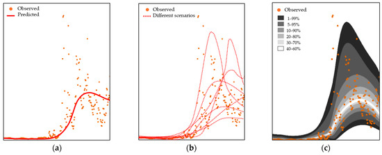
Figure 1.
Examples of (a) deterministic prediction, (b) ensemble prediction, and (c) probabilistic predictions. Bands indicate the percentage of observations expected to fall within their bounds.
This study investigates the application of a deep learning model, the Temporal Fusion Transformer (TFT) [17], to perform probabilistic forecasts of hourly potential hydropower production in the run–of–the–river hydropower plant of Covas do Barroso, in Portugal. The TFT is a recent deep learning model specialized in time series forecasting that combines the strengths of Long Short–Term Memory (LSTM) [18] with self–attention (transformer architecture) [19]. The former has gained traction within the hydrological community (e.g., [20]), and their performance is improving to the point of challenging long–held beliefs about the need for physically and/or conceptually based hydrological models [21]. The latter has been instrumental in the development of Large Language Models (LLMs), achieving state–of–the–art performance across numerous natural language processing tasks, including machine translation, text summarization, and conversational.
The analysis is based on earlier work, where TFTs were already applied to predict daily streamflow with satisfactory results [22]. Notably, in the task of rainfall–runoff modeling, TFTs surpassed the performance of the classical Hydrologiska Byråns Vattenbalansavdelning (HBV) model [23]. Here, the focus is somewhat different, with emphasis on forecasting hourly potential hydropower production. To that end, an analysis of the influence of meteorological forecasts from two main sources was first compared: the European Centre for Medium–Range Weather Forecasts (ECMWF), and the Global Forecast System (GFS). Secondly, historical hydropower production records were pre–processed to filter out human “interference” and account for modifications in the infrastructure (e.g., increases in installed capacity over time). Finally, a TFT model capable of forecasting potential hydropower production intended for use in the day–ahead spot market was trained and evaluated.
The manuscript is structured in the following sections:
- Introduction (Section 1);
- Section 2 is dedicated to describing the case study—the Covas do Barroso small hydropower plant;
- Section 3 describes the adopted methodology, with emphasis on the workflow;
- Results and discussion are addressed in Section 4;
- Main conclusions are drawn in Section 5, along with propositions for future work.
2. Case Study
The Covas do Barroso run–of–the–river hydropower scheme is located in the northern region of Portugal, in southwestern Europe (Figure 2a), more specifically, in the municipality of Boticas, in the district of Vila Real. It is and has been in operation since 1996 [24]. Inflows to the powerhouse come from two weirs built on the Covas River and the Couto River. Illustrated in Figure 2b, the catchment under study has an area of 80.2 km2, corresponding to 58.9 km2 on the Couto River (West) and 21.3 km2 on the Covas River (East). The average annual precipitation in the region was estimated at 1750 mm, and the average annual flow was quantified at 3.33 m3/s. Figure 3 shows a schematic representation of the hydropower scheme. Although it is a run–of–river scheme, its operation follows a “pond–and–release” regime, based on the available storage capacity along the channel, particularly when natural streamflow falls below the turbines’ minimum allowable flow. The channel’s storage capacity is approximately 3000 m3. The scheme also includes priority discharge systems for ecological and irrigation purposes. The scheme is owned by the private Portuguese company Lusiterg—Gestão e Produção Energética and operated under an O&M services rendering contract by Hidroeg —Projectos Energéticos, also a Portuguese company responsible for building, managing, and operating power facilities designed to produce electricity from renewable energy sources [24].
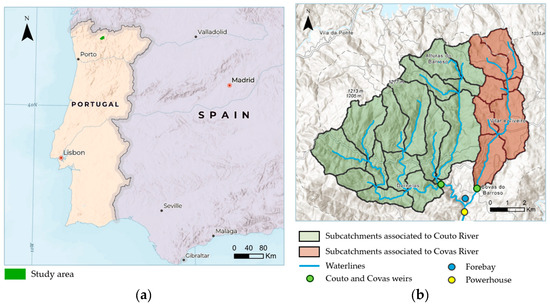
Figure 2.
Study area overview: (a) a map of Portugal highlighting the location of the study area (in green); and (b) the catchment of the Covas de Barroso hydropower plant (HPP), including its tributaries (depicted in blue), their respective catchments (outlined in black), and other HPP’s components.
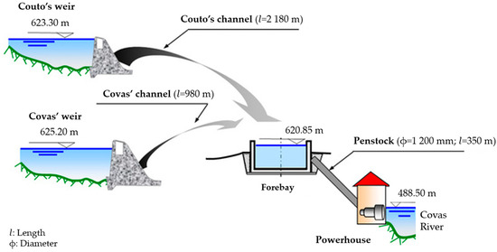
Figure 3.
Schematic representation of the hydropower scheme of Covas do Barroso. Adapted from [24].
The powerhouse is equipped with two identical Francis turbines, designed for a gross head loss of 132.75 m. The maximum total turbined flow rate is 5.70 m3/s. The average equivalent useful head is approximately 130.10 m, corresponding to a total installed power of 6.4 MW and an estimated average annual energy production of 15.2 GW.
The streamflow that exceeds the capacity of the water intakes of the weirs on the Couto or Covas rivers is spilled over their respective weirs, bypassing the hydraulic system. Because the streamflow over the weirs is not available, there is no way to monitor high streamflow, directly or indirectly, posing a challenge to model calibration. Predicting potential hydropower production directly—without working previously on water flow and converting them to power output—makes it possible to overcome that limitation.
3. Methodology and Data Characterization
3.1. Overview
The adopted methodology was designed to address the key challenges of hydropower forecasting using ML techniques. As laid out in the introduction, there are three main parts to this work:
- (1)
- Data collection, validation, pre–processing, and feature engineering. The most significant part in this step was the removal of human “interference” in the hydropower production data.
- (2)
- Comparison of different sources of meteorological data. Here, data from ground, reanalysis, and forecast sources were compared.
- (3)
- Deep learning model development to forecast hourly potential hydropower production at the Covas de Barroso scheme.
Naturally, steps (2) and (3) entailed performance assessments, in turn to objectively compare the quality of the different meteorological data and to develop and validate the forecasting model.
Step (3), synthesized in Figure 4, required feature engineering as a means to the generation of informative inputs to the model and the tuning of the TFT network architecture and hyperparameters. Usually, this is an iterative process which involves tuning the hyperparameters (external configuration variables used to manage model training), such as learning rate, batch size, and dropout rate. It also involves defining training and validation processes (calibration), with a particular focus on preventing overfitting. In this study, this aspect was not explored in depth, relying instead on gained insights from existing literature and previous research.
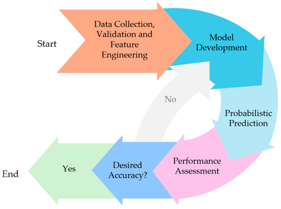
Figure 4.
Adopted methodology for model development. As referred, the recursive nature of the hyperparameter optimization process was not explored in full detail. Consequently, this part of the methodology is depicted in a lighter color to indicate its reduced emphasis here.
To inspect the TFT’s performance, development was undertaken in two steps. First, a “pseudo–forecasting” model was trained. Here, the model presented information on hydropower production up to the forecast preparation time, as well as access to “known” meteorological data from ERA5–Land covering and future time steps. On a second step, real forecasts were made, using meteorology from ECMWF and the GFS (as there are insufficient forecasts available in time to train the TFT directly with forecasts). Doing so entailed intermediate actions:
- (1)
- Linear adjustment of ECMWF and GFS data to ERA5–Land conditions. In case of temperature, achieving the same mean and standard deviation. In the case of precipitation, obtaining the same mean. Corrections were based on the civil year of 2022. We applied similar corrections to the previous work [22].
- (2)
- Hiding information not known at the time of operational decisions. For practical purposes, placements of hydropower in the day–ahead market must be made during the afternoon (assumed as 4 PM in the case of this work). This means that, at the time of the decision, meteorological forecasts used for the day–ahead are approximately 16 h old (00:00 UTC cycle), and their effective lead times range from 24 to 48 h.
All predictions were made with an hourly time step.
The work conducted on TFTs represents a follow–up of a previous publication that applied them to streamflow prediction [22]. There was an effort to avoid redundant aspects, particularly in the methodology, but also to provide the necessary information for the reader to follow this work independently.
3.2. Data Collection, Validation, and Feature Engineering
3.2.1. Potential Hydropower Production Data
The hydropower production data analyzed at Covas do Barroso spans the period from 2006 to 2023. The data kindly provided by Lusiterg—Gestão e Produção Energética were nearly complete, which was highly beneficial as the availability of continuous data is helpful to ensure that the predictive model learns effectively. The time step of the original records was 15 min, then aggregated to hourly values.
The major challenge associated with these data, not usually present in similar cases focusing on streamflow, is bound to the various constraints from technical and human nature that influence production (e.g., outliers caused by the start and interruption of operations, other random errors, long–term updates to the infrastructure, electromechanical issues and planned maintenance, limitations of the electricity grid, and intermittent “pond–and–release” operations during low flows). While most of these outliers reflect physical and operational processes, occasional sensor inaccuracies, data logging inconsistencies, or supervisory control and data acquisition (SCADA) system malfunctions may also contribute. These can lead to discrepancies between the potential and the actual hydropower output. Here, effects were analyzed and handled individually. Data pre–processing was undertaken in three main steps:
- (1)
- Low–flow filter to remove the effect of “pond–and–release” operations.
“Pond–and–release” operations are undertaken due to limitations in the minimum streamflow allowed through the turbines (Figure 5a). When inflows fall below that threshold, a small volume available along the conveyance channels and forebay is used to store water so that one turbine may function, though for a short period, at its minimum nominal flow.The conveyance channels and forebay were designed to provide a storage capacity compatible with a maximum of 5 to 6 turbine startups. Once the stored water is exhausted, operations stop, and the process of refilling them is restarted. In the case of Covas do Barroso, turbines should not operate significantly below 1.20 to 1.25 MW.
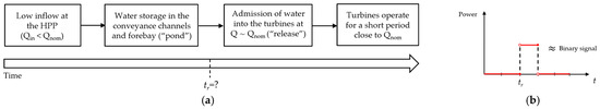
Figure 5.
Rationale behind the low–flow filter: (a) process of “pond–and–release” and (b) representation of this operation with “release” at tr for a short period of time. Here, Qin is the inflow in the HPP, Qnom is the nominal flow of turbines, and tr the instant of “release”. The red line represents the relative variation in hydropower output over time in a “pond–and–release” operation.
Once the system enters the “pond–and–release” operation, it is necessary to decide on the instant of “release” (tr). This is dependent on several factors, such as the nominal flow of turbines (Qnom), inflow (Qin), financial penalties in the energy market, and submitted generation bids. Trying to predict the exact timing of power production resulting from the combination of these variables can be complex. Besides that, the output in these cases is similar to a binary signal (turbining close to Qnom or not turbining, Figure 5b). Making the TFT (and other deep learning models) predict power output during “pond–and–release” can heavily deteriorate the quality of the results over the time series. Applying a filter overcomes this problem by transforming the data (intermittent signal) into inflow. In this way, the TFT focuses on providing useful information into the normal operational regime, and the complex task of scheduling under “pond–and–release” is left to the operators.
The filtering operation, whose result is illustrated in Figure 6, was accomplished as follows:
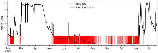
Figure 6.
Illustration of the effect of the low–flow filter to remove the effect of “pond–and–release” operations.
- Creation of a binary series where ones (1) represent turbining and zeros (0) represent no turbining. A threshold of 0.5 was used (comfortably below the minimum operation setting of the turbines);
- “Forward” pass filtering of the binary series, where the average fraction of time between “pond–and–release” cycles is calculated. Averaging is performed from the end of one cycle to the end of the following one;
- “Backward” pass filtering of the binary series, where the average fraction of time between “pond–and–release” cycles is again calculated. Now, averaging is performed from the start of one cycle to the start of the following one;
- Averaging of the “forward” and “backward” series and applying a rolling window of 4 days for smoothing (the long window is justified by the relative stability of low flows, which typically correspond to dry catchment conditions. These results in the fraction of the time the powerhouse was effectively in operation;
- Calculation of the “pond–and–release” setting over time and smoothing with a rolling window of 4 days. Obtains values close to the aforementioned 1.20 to 1.25 MW interval;
- Multiplication of the fraction of the time of effective powerhouse operation by the time series of “pond–and–release” settings obtained in the previous two steps;
- Replacement of raw “pond–and–release” data within the complete power output series by the potential production series obtained above.
- (2)
- High–flow filter to remove outliers.
Next, the evident presence of outliers in the production time series had to be dealt with. To do so, a so–called high–flow filter procedure was implemented as follows:
- Calculate the absolute difference between the low–flow filtered series and a smoothed signal defined as the average of forward and backward exponential moving windows (span of 8 steps, or 2 h);
- Select periods where the difference is greater than a certain threshold (0.2 MW was assumed) as an indication of outliers;
- Prolong outlier events. After applying a centered rolling maximum (span of 4 steps, or 1 h), prolong events until 95% of the power generation before the start of the event or a fixed threshold of 4 MW was surpassed up to a maximum duration of 2 days. Refer to Figure 7 for an illustration;
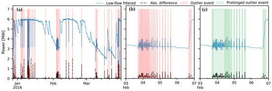 Figure 7. Illustration of the intermediate steps of the high–flow filter for outliers: (a) example of selection of outlier periods; (b) detail of February 2016; (c) and detail of prolonged outlier events in February 2016.
 - Erase outlier periods and linear interpolation of the erased data on the log–log space, resulting in a corrected time series of potential hydropower production where the impact of “pond–and–release” operations is not felt, and outliers were removed (Figure 8).
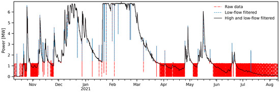 Figure 8. Illustration of the combined effect of the low–flow and high–flow filters.
- (3)
- Accounting for changes in installed capacity.
In 2013, the installed capacity at Covas do Barroso was increased from 5.8 to 6.1 MW. In 2019, another upgrade was made, updating that value to 6.4 MW. Finally, in 2020, a capacity of 6.7 MW was reached. To train the TFT, a series representing these changes was included as an additional exogenous input. In detail, to also account for smaller, continuous fluctuations in the status of the hydropower scheme (e.g., due to equipment settings and wear and tear, resistance to the flow in hydraulic circuits, changes in the rating curve of the river at the outlet of the powerhouse, etc.), a continuous series representing actual installed capacity was used. That series was built by retrieving the maximum power output of every hydrological year and associating it with the start of the matching period (the 1st of October, prior to the onset of the wet season). Values for all remaining dates were estimated by linear interpolation (Figure 9).
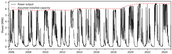
Figure 9.
Filtered power output records at Covas do Barroso and assumed time series of installed capacity.
3.2.2. Meteorological Data
Potential hydropower in run–of–the–river schemes is strongly linked to available streamflow. In turn, streamflow is heavily dependent on the hydrological state of the contributing catchments (e.g., soil moisture, infiltration) and meteorology. Consequently, the quality of the meteorological data can greatly affect the quality of potential hydropower predictions. With the previous assertion in mind, several sources of meteorological data (precipitation and temperature) were considered:
- Ground–based observations:
- (i)
- From the Portuguese National Water Resources Information System (SNIRH): For this project, hourly precipitation data were collected from the SNIRH [25] at rain gauges in Vila da Ponte, Telhado, Alturas do Barroso, Vilar do Porro, Salto, and Couto de Dornelas, all located within or close to the catchment under study (Figure 10). Of those records, Vila da Ponte, Telhado, and Salto appeared to be of higher quality, having time series with fewer gaps, showing precipitations of similar magnitude, and evidencing a synchronicity of events that should be expected of nearby gauges. Accordingly, more attention was given to them. The analyzed data covered the period spanning from 2015 to 2023.
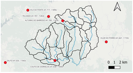 Figure 10. Location of the rain gauges considered near the catchment of Covas do Barroso hydropower plant, with the respective coordinates (latitude, longitude) in the WGS84 (EPSG:4326) datum.
 - (ii)
- From ERA5–Land: ERA5–Land reanalysis data [26] were also used to characterize hourly temperature and precipitation. These data, produced by the European Centre for Medium–Range Weather Forecasts (ECMWF), were aggregated for the studied catchment and adjusted to the national time zone. Generally, regarding precipitation, ERA5–Land data have the advantage of high consistency over time, without gaps, convenient temporal discretization (hourly), and relatively detailed spatial resolution (0.1 × 0.1° grids).
Figure 11 compares precipitation measurements from SNIRH (for Salto, Telhado and Vila da Ponte) and ERA5–Land for November 2020 in the studied catchment. As can be seen, although the evolution of the precipitation in both sources is similar, ERA5–Land misses some precipitation peaks (e.g., between 21 and 25 November 2022).
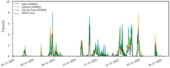
Figure 11.
Comparison of the observed values of precipitation from SNIRH and ERA5–Land in the in–study catchment, in November 2022.
Moreover, looking at the cumulative series of precipitation from both sources (Figure 12), the largest deviations in ERA5–Land values happened during spring (May and June) with the accumulation of events that were not registered by the rain gauges. To facilitate the joint analysis of cumulative and instantaneous values, Figure 13, focusing on November 2022, was also included below.
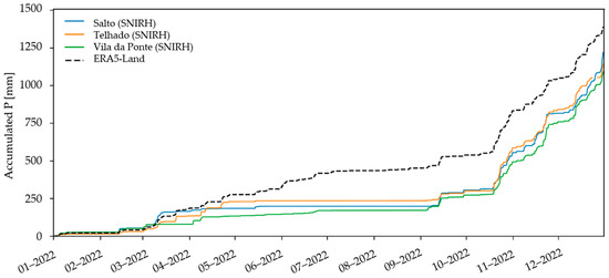
Figure 12.
Comparison of the cumulative series of precipitation from SNIRH and ERA5–Land in the in–study catchment during the civil year of 2022.
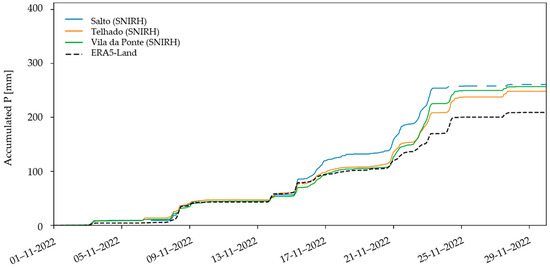
Figure 13.
Comparison of the cumulative series of precipitation from SNIRH and ERA5–Land in the in–study catchment during November 2022.
- Forecasts:
- (i)
- From the ECMWF: ECMWF ensemble forecasts [27], which are reputed for their comparative accuracy worldwide (e.g., [28,29]), were shared by the Portuguese Institute for Sea and Atmosphere (IPMA) for the purposes of this study. The data corresponds to an ensemble of forecasts covering the civil year of 2022. The details are a 5–day forecast horizon and a tri–hourly time step, with spatial discretization of 0.10 × 0.10°.The ECMWF data corresponded to the 00:00 UTC production cycle and precipitation were pre–processed for the studied catchment from 1 January 2022 forward. After spatial aggregation, they were resampled to hourly time steps: temperature linearly and precipitation in 3 equal values for each 3 h block. Finally, the time zone was updated to local time.A comparison of ECMWF data with ground observations is presented in Figure 14, which contains forecasts for a lead time of 0 days and forecasts for a lead time of 3 days (the forecast lead time is progressive, and the reference lead time is relative to the 00:00 UTC cycle. In the case of “ECMWF 0 days” data, end–of–first–day forecasts have lead times closer to 24 h. In the case of “ECMWF 3 days” data, end–of–first–day forecasts have lead times closer to 60 h). Time series are shown with individual ensemble members represented in gray, and the ensemble average is represented by the black dashed line. The degradation of forecast quality with increasing lead time is evident, both in terms of increasing uncertainty and the inability to accurately predict the timing of some events (e.g., 8 November 2022).
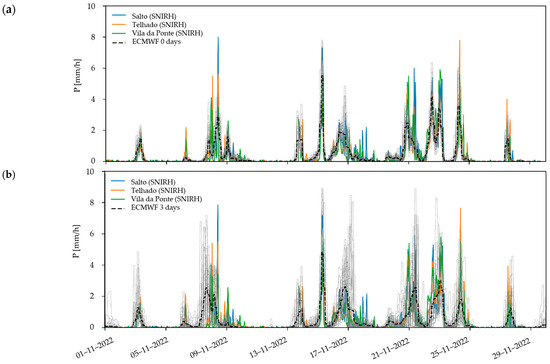 Figure 14. Comparison of the ECMWF forecasts with SNIRH data for November 2022, namely (a) same–day forecast and (b) 3–day forecast. Individual ensemble members are shown in gray. Ensemble average is shown by the black dashed line.That said, it is also fair to mention that the overall precipitation variation is well captured. Indeed, the high quality of the forecast is also visible through the comparison of the accumulated precipitation series (Figure 15), where the ECMWF forecast appears to be superior to the ERA5–Land data (see Figure 13). In the following analysis, only the average value of the ensemble is considered.
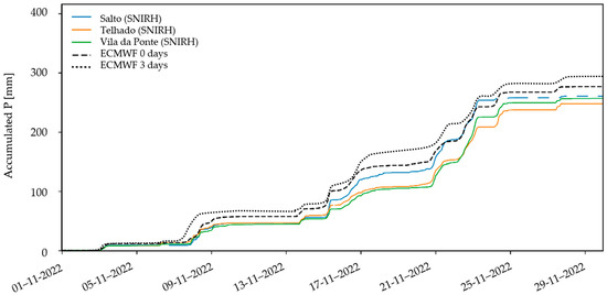 Figure 15. Comparison of the cumulative series of precipitation from rain gauges (SNIRH) and the average of ensembles from the ECMWF, for same–day and 3–day forecasts, in the studied catchment, in November 2022.
 - (ii)
- From the GFS: Alongside the ECMWF product, GFS, from the US National Centers for Environmental Prediction (NCEP), is a global weather forecasting model [30]. Compared to the former, it has the advantage of being publicly available. However, the entire ECMWF real–time catalog will be fully and freely available under a CC–BY–4.0 license starting 1 October 2025. On the other hand, its performance is arguably worse. The GSF forecasts corresponding to the 00:00 UTC production cycle have a 3 h time step, being prepared in 0.25 × 0.25° grids. They were also adjusted to the national time zone and aggregated for the catchment of Covas do Barroso.A comparison of GFS forecasts with ground observations is performed in Figure 16. Again, the 3–day lead time forecast is clearly worse than the same–day forecast, which is a reasonable finding. More informatively, the GFS forecasts appear less accurate than the ECMWF.Regarding the accumulated values (Figure 17), it can be highlighted that the behavior is satisfactory. Contrary to what would be expected, the accumulated values at different horizons change markedly (this observation is also valid for extended periods and other regions). This hints at a potential bias in the forecasts that is a function of lead time.
3.3. Model Development for Potential Hydropower Production Forecasting
Previous state–of–the–art studies have surveyed the potential of various deep learning models for hydrological applications. For example, Farfán–Durán and Cea [31] concluded that recurrent neural networks (RNNs), such as gated recurrent unit (GRU) and LSTM, can outperform convolutional neural networks (CNNs) in streamflow prediction and shorter lead times.
The Temporal Fusion Transformer (TFT) is a deep neural network apt for complex, multi–horizon, and multivariate time series problems. It is a powerful “tool” for prediction tasks based on observed tendencies [17]. Based on the “transformer” design (self–attention) [19] and LSTM [18], TFTs contain several features that are particularly interesting when working on time series (Figure 18).
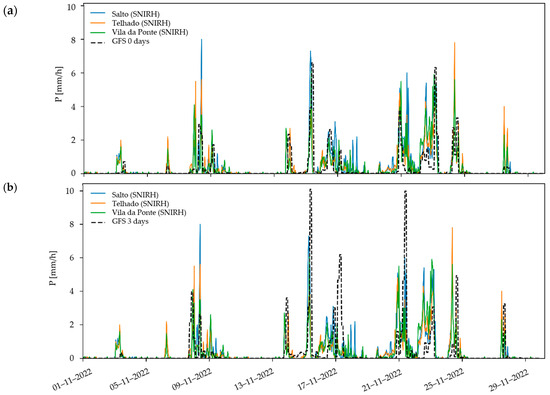
Figure 16.
Comparison of the GFS forecasts with SNIRH data for November 2022, namely (a) same–day forecast and (b) 3–day forecast. Ensemble average shown by black dashed line.
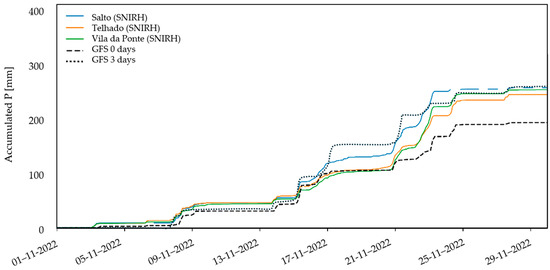
Figure 17.
Comparison of the cumulative series of precipitation from SNIRH and the average of ensembles from GFS, for same–day and 3–day forecasts, in the studied catchment, in November 2022.
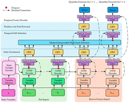
Figure 18.
TFT architecture overview. The model incorporates static variables, past inputs, and known future inputs, with a focus on dynamic variable selection. The gated recurrent networks (GRNs) are used to enhance the model’s ability to capture temporal dependencies. S represents the static variables, denotes the time series inputs, t is the current instant in analysis, k is the number of instants preceding t, and n is the forecast horizon. Adapted from [17].
Generically, TFTs are composed of the following:
- (1)
- Variable selection networks, dynamically selecting relevant input variables at each time step, enhancing interpretability and efficiency;
- (2)
- Static variable encoders that are used for processing static features that remain constant over time;
- (3)
- Encoder–Decoder LSTMs, which capture temporal dependencies by processing past and future variables separately, with encoders and decoders, respectively;
- (4)
- Multi–head attention, enabling the model to focus on different aspects of the input sequence for improved forecasting;
- (5)
- Residual connections, dropout, gates, and normalization. These techniques help enhance training and generalization ability, as well as prevent overfitting.
For more specific details about TFTs, please consult the work of Lim et al. [17].
Koya and Roy [32] demonstrated that TFTs can surpass LSTM and Transformer models in streamflow prediction. Therefore, TFTs were chosen as the deep learning model for hydropower production, as hydropower generation is significantly dependent on streamflow, as previously mentioned.
The modeling process was conducted in Python 3.9.18 (December 2023) using the PyTorch v.2.5.1 library and the PyTorch Forecasting v.1.1.1 package [33]. The adopted integrated development environment (IDE) was Eclipse (with the PyDev extension).
As inputs, hourly precipitation, temperature, and assumed installed capacity (as mentioned in Figure 8), total hours since the start of the time series, and two–yearly cycles (sine and cosine with a period equal to the total number of hours in a year) were added. No static covariates were considered in this work. The target was the potential hydropower after pre–processing.
In the previous study [22] (more details on the model can be found there), we have explored TFTs for the similar problem of streamflow prediction and strengthened domain–specific knowledge on the effect TFT hyperparameters (e.g., learning rate, dropout rate, hidden size, patience). In this case, additional preliminary simulations were conducted to fine–tune the architecture of the network (e.g., number of hidden neurons, attention heads, and LSTM layers) to the prediction of hourly potential hydropower production. For each simulation, the available data were divided into training, validation, and test periods, as is common practice in ML applications. The division of the full analysis period (2015–2023) was constrained by the availability of ECMWF forecasts covering only the civil year of 2022, which was accordingly “saved” for testing. Validation spanned from October 2020 to December 2021 (the start of this period in October is justified by the hydrological year, which, in Portugal, is defined from 1 October to 30 September). The remaining data were used for training.
The training process of the TFT was guided by minimizing the quantile loss function, using the Ranger optimizer [34]. To ensure stable convergence, we employed a learning rate decay strategy in which the learning rate was gradually reduced by a factor of 10 at each 4 epochs of training. The initial learning rate was set to 0.0001. This approach prevents oscillations in weight updates and accelerates convergence toward an optimal solution.
To assess convergence, we monitored the validation loss over successive epochs and employed an early stopping criterion with a patience parameter of 14 epochs. Training was halted to prevent overfitting and unnecessary computational work if the validation loss did not improve within this window. Additionally, we applied dropout regularization of 30% to enhance generalization performance, and block overfitting as well.
Empirically, we observed that our model converges within approximately 30–40 epochs for the specifications in Table 1. Table 1 presents the adopted hyperparameters in the final TFT model. More information on the denotation of each hyperparameter is available on PyTorch Forecasting v1.1.1 [33,35] and PyTorch Lightning v1.9.4 [36] documentation.

Table 1.
Adopted hyperparameters in the final TFT model.
3.4. Performance Assessment
3.4.1. Deterministic Predictions
The simplest error metric used here is the mean absolute error (MAE)—Equation (1). Its optimal value is 0 and has data units. The larger the disparities between observed and predicted values, the larger the MAE.
Above, is the time step, is the total number of time steps considered, is the observed variable at the th time step, and is the predicted variable at the th time step.
The Nash–Sutcliffe efficiency (NSE) [37] is a popular metric to assess the performance of deterministic models, particularly among the hydrology community. It is scale invariant, and the optimal value is 1. It can be calculated through Equation (2):
where additionally to the description of the previous variables, is the sample mean of the observed variable.
The Kling–Gupta efficiency (KGE) metric was proposed by Gupta et al. [38] and presents an alternative to the NSE. It can be calculated according to Equations (3)–(6). It is also dimensionless, and its optimal value is also 1.
Increasing deviations between the observed and predicted values decrease the value of both NSE and KGE.
Above, in addition to the previous definitions, is the Pearson correlation coefficient, the sample mean of the predictions, the sample standard deviation of the predicted variable, and the sample standard deviation of the observed variable.
In the results presented below, deterministic performance metrics calculated for probabilistic (TFT) and ensemble (ECMWF and GFS) time series are always computed based on expected values.
3.4.2. Probabilistic Predictions
The Continuous Ranked Probability Score (CRPS) [39] can be used to evaluate the performance of deterministic, ensemble, and probabilistic predictions, being, in that regard, extremely versatile. It has the data units and is defined by Equation (7):
where is the value of the cumulative distribution function of the predicted variable at the th time step, and is the Heaviside step function.
A perfect prediction results in a CRPS of 0. When used to assess deterministic predictions, the CRPS can be simplified to the MAE. It can, therefore, be used to compare directly probabilistic, ensemble, and deterministic predictions (in detail, a correction can be applied to the CRPS that accounts for the number of ensemble members. See [39] for more details).
Predictive quantile–quantile (QQ) plots are grounded on the quantile distribution of the observed and predicted variables and were used here as a basis for evaluating reliability ()—Equation (8) [40]. Reliability consists of the complementary area between the obtained QQ plot for the prediction and a perfect diagonal (Figure 19). Deviations from the diagonal reflect different types of shortcomings in predictions. Values of equal to 1 are desired [40]. It is also a dimensionless variable.
Above, is the p–value of the th ranked prediction, and is the theoretical p–value of the th ranked prediction.
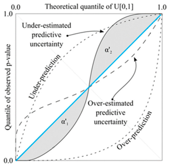
Figure 19.
QQ plot and respective interpretation concerning probabilistic predictions. The diagonal (blue line) represents the desired reliability line. Adapted from [40].
Because reliability is largely decoupled from the “magnitude” of the predictive uncertainty, it is useful to combine it with additional metrics that evaluate the sharpness or resolution of the prediction. The relative resolution (), expressed in Equation (9) and usually in the data units, is a straightforward way to do so [40]. The smaller the “width” of the predictive uncertainty, the greater the relative resolution.
In the above equation, is the sample standard deviation of the predicted streamflow at the th time step.
4. Results and Discussion
4.1. Comparison of Meteorological Data Sources
Following the analysis of meteorological data, some observations can be made based on a comparison of model performances computed for the civil year of 2022 (common period of all datasets):
- The ECMWF temperature forecasts are closer to the reference (ERA5–Land) than the GFS ones, as consistently evidenced in Figure 20 for different lead times and perfomance metrics. This is supported by the fact that, in relation to GFS, ECMWF’s CRPS and MAE are lower and KGE and NSE are higher.
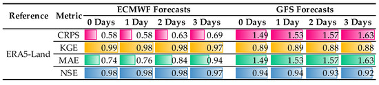 Figure 20. Performance metrics for different temperature data. The color bars are proportional to the values in each metric.
 - ECMWF precipitation forecasts outperform GFS forecasts when compared with the records from the Salto and Telhado rain gauge stations, as sustained by Figure 21.
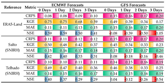 Figure 21. Performance metrics for different precipitation data. The color bars are proportional to the values in each metric.
 - The degradation of ECMWF precipitation forecasts with increasing forecast lead times is significant. However, at least up to the 3–day horizon, this degradation is not yet complete (see Figure 21).
- The value of GFS precipitation forecasts over Covas do Barroso is questionable, regardless of the considered lead time (see, for example, the NSE values presented in Figure 21).
4.2. Pseudo–Forecasting of Hourly Potential Hydropower Production
Focusing on hourly potential hydropower production, a TFT model was trained in the framework of a “pseudo–forecasting” task. In this case, the inputs are the latest “observed” potential hydropower production plus “known” meteorology from ERA5–Land.
The full results for a 1–day forecast horizon are illustrated in Figure 22, referring to the total analysis period and where the training, validation and testing periods are identified. It should be noted that this is a case “halfway” between simulation and forecasting (thus, denominated “pseudo–forecasting”). Numerical results are presented in Figure 23. Naturally, performance is degraded with increasing lead time. Climatology and persistence are used as benchmarks. The former represents the long–term distribution of the variable as a function of the time of the year, while the latter consists of the last recorded value being propagated forward in time. Climatology metrics are independent of lead time. Persistence values are particularly good for very short lead times, degrading rapidly. It is interesting to remark that the performance of the TFT generally falls between them both.
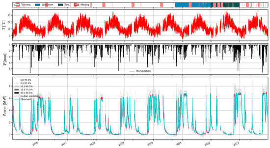
Figure 22.
Simulation with known effective power (1–day lead time), for the complete period from 2015 to 2023. ERA5–Land precipitation and temperature were used as input.
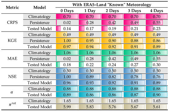
Figure 23.
Performance metrics for the pseudo–forecasting of potential hydropower production. Color bars are proportional to the values of each metric. Civil year of 2022.
One aspect of the performance metrics that should immediately catch the attention of the reader is that TFT performances for the lead time of “0 days” (the shortest lead time possible—1 h) are markedly inferior to the one achieved by the persistence benchmark. Without context, that is strange because the TFT could “easily” assume persistence for short lead times and transition to more elaborate “rainfall–production” transformations as the lead time increased. Obviously, that was not the case. Instead, the TFT models that were tested tended to err more on the side of the “rainfall–production” transformations, effectively almost neglecting the latest observed production records.
The reason for this counterintuitive behavior lies in the relatively long horizon of the forecasts, which span over 120 hourly time steps. The loss function that was used—quantile loss—steers the backpropagation process by averaging quantile losses computed over the full forecasting horizon. When the autocorrelation in the series affects only a relatively short number of time steps over the whole forecasting horizon, that information is diluted and not picked up by the network. Indeed, when the same model is trained for a shorted horizon which is, in its entirety, affected by autocorrelation, the TFT relies on it instead of meteorology to make predictions.
4.3. Forecasting of Hourly Potential Hydropower Production
Both forecasts with ECMWF and GFS data were performed in an operational setting (the model has information about the potential hydropower) based on the information known at 4 PM on the day the forecast is issued. As an example, the results of a forecast made at 16:00 on October 8 are presented as follows:
- 1–day horizon: potential powers from 00:00 to 23:00 on 9 October;
- 2–day horizon: potential powers from 00:00 to 23:00 on 10 October;
- So forth until a 4–day horizon to ensure next–business–day predictions in the case of a weekend following a holiday (or vice versa).
Figure 24 shows detailed forecasts for the months of November and December 2022, obtained for horizons of 1, 2, 3, and 4 days with ECMWF data. Observations about these forecasts can be made:
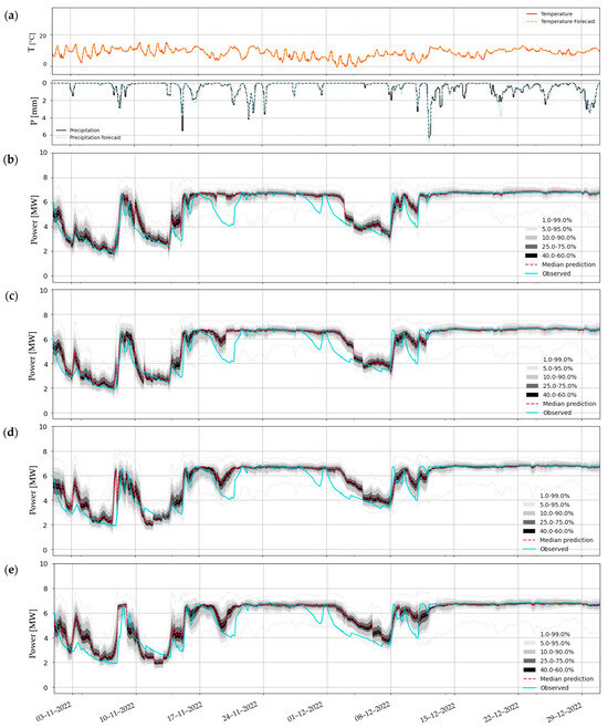
Figure 24.
Set of probabilistic predictions of potential hydropower production at Covas do Barroso, for November and December 2022: (a) meteorological forecasts (ECMWF), and horizons of (b) 1, (c) 2, (d) 3, and (e) 4 days.
- The TFT was able to effectively identify the moment of increases in potential power, particularly for the 1– and 2–day forecast horizons (e.g., 8 November 2022, 15 November 2022, 8 December 2022). However, there is room for improvement in the model’s ability to reproduce power decreases, as demonstrated on dates like 20 November 2022 and 30 November 2022.
- Predicted (dashed light blue line) and observed (black line) precipitations are satisfactorily accurate for the represented period (see Figure 24a).
Below, in Figure 24, meteorological forecasts for the months of November and December are presented, as well as hydropower forecasts from GFS data sources, corresponding to the different forecast horizons. Some observations about these forecasts are as follows:
- There are clear discontinuities from one day to the next in the forecasts (something that in the previous forecasts was not that flagrant). This is because the forecasts are not “continuous” for a given horizon but are updated daily with new meteorology data. As such, they correspond to a discontinuous horizon. What is here, for convenience, called the “1–day horizon” actually consists of forecasts with horizons varying between 8 and 31 h. Something similar happens for the other horizons;
- There may be significant disparities between predicted (dashed light blue line) and observed (black line) precipitation, even for the 1–day horizon (see Figure 25a);
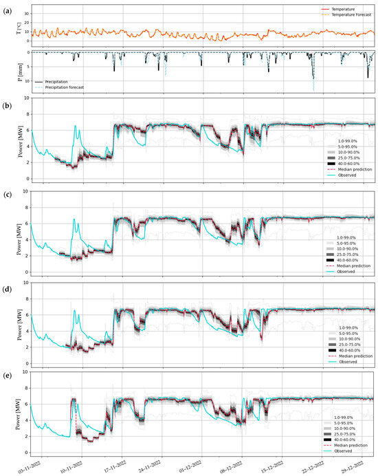 Figure 25. Set of probabilistic predictions of potential hydropower production at Covas do Barroso, for November and December 2022: (a) meteorological forecasts (GFS), and horizons of (b) 1, (c) 2, (d) 3, and (e) 4 days.
 - Here, the TFT model fails to capture most of the potential hydropower observed between 8 and 15 November, and between 6 and 12 December. Forecasts based on GFS data are far from perfect, and less accurate than the ones produced with ECMWF data, solely based on the presented plots. This is likely largely due to the lower quality of precipitation forecasts (as sustained previously by Figure 20).
Performance metrics are presented in Figure 26 for the TFT model with forecasts from ECMWF and GFS. Additionally, for benchmarking purposes, metrics associated with climatology (historical variability of the series on each day of the year) and persistence (which assumes forecasts equal to the last observed value) were included. Thus, the following can be considered the main findings:
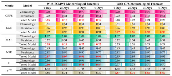
Figure 26.
Performance metrics for potential hydropower forecasting models. Color bars are proportional to the values in each metric. The best alternative for each horizon and metric is marked in bold red font.
- As expected, after analyzing the meteorological forecasts and the plots, power forecasts with ECMWF meteorological information are more accurate. However, the model has some shortcomings regarding the KGE. Interestingly, it is noted that the relative deviation (inversely proportional to relative resolution) is smaller when the same TFT is fed with GFS data. This fact clearly indicates that the source of the deviation is the weather forecasts. If it is persistent, it can be partially corrected through a simple linear transformation;
- As expected, after analyzing the graphs of the various forecasts, it can be argued that the TFT model fed with ECMWF data achieves the best performance (CRPS, MAE, and NSE).
Figure 27 depicts the QQ plots for operational potential hydropower forecasts from ECMWF and GFS data. As previously mentioned, the former achieved higher resolution and reliability, also supported by Figure 27a. Also, from the shape of the QQ plots, it can be ascertained that both models have some tendency toward underprediction, particularly GFS’.
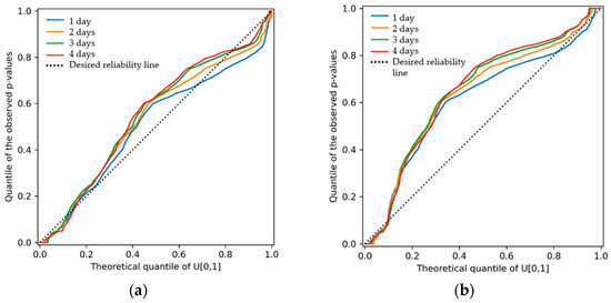
Figure 27.
QQ plots for operational potential hydropower forecasts based on (a) ECMWF and (b) GFS data at different forecast horizons.
Despite the encouraging results, there are several obstacles to the practical application of the methodology described that we believe are worth addressing:
- (1)
- Data quality and availability: A significant challenge for any ML model is the quality and availability of data. Using reliable meteorological sources like ECMWF precipitation forecasts and reanalysis data can help address this concern, as well as the plant’s historical production data;
- (2)
- Integration with existing systems: Incorporating TFTs into current hydropower plant management systems can be complex, particularly as these systems were not originally designed for ML integration. As ML becomes more dominant and accessible, we believe the proposed framework can be gradually introduced alongside existing systems;
- (3)
- Interpretability and trust: One of the main concerns with ML models is that they are often seen as “black boxes”, making it hard for operators to “trust” their predictions. The attention mechanisms can highlight which factors—like meteorological data and past production records—influence the model’s decisions (through the attention scores);
- (4)
- Computational resources and ongoing maintenance: Implementing a ML–based forecasting system requires investment in both software and hardware. Plus, these models need continuous maintenance—like retraining with new data and tuning hyperparameters—to stay accurate, requiring specialized expertise in ML.
5. Conclusions
After a detailed assessment of the quality of meteorological data and the implementation of two models for forecasting potential hydropower production at the Covas do Barroso run–of–the–river small hydropower plant, in northern Portugal, several key insights have been identified:
- Superior accuracy of ECMWF: ECMWF meteorological forecasts of temperature and precipitation are more accurate than GFS forecasts. Focusing on precipitation, ECMWF’s product comes closer to ground–based data;
- Effectiveness of the TFT model: the TFT model, especially when combined with ECMWF forecasts, can satisfactorily forecast potential hydropower production, outperforming forecasts made based on GFS data;
- Potential for operational application: the results suggest that the TFT model presents a promising avenue for operational forecasting in Covas do Barroso and similar hydropower schemes, paving the way for enhanced decision making and more rationalized use of renewable energy resources. This said, despite a confirmed capacity to predict the ascending “limb” of the production following rainfall events, there is still a significant margin for improvement. Such improvements may be achieved through several axes of research, some of those being (i) modifications in model training aiming to focus the “attention” of the TFT to short and long lead times alike, possibly by using a custom loss function; (ii) further enhancing the choice of hyperparameters; or (iii) exploring other sets of inputs.
To undertake the analysis, it was necessary to pre–process the time series of actual hydropower production records with filtering operations of some complexity. The description of those operations, aiming at removing the effects of “pond–and–release” operations, outliers, and generally unpredictable anthropogenic influence, may be useful to other researchers and/or practitioners.
As a final note, it can be emphasized that the application of ML models such as TFTs is very practical and achieves satisfactory performance. For example, to model hydropower production within a physically based framework would entail the simulation of hydrology, the hydraulic system of the scheme, and the operational features of the electromechanical equipment involved in hydropower production. On the contrary, TFTs can bypass that considerable complexity and be used to predict the variable of interest directly.
Author Contributions
R.F., R.M. and J.P.M. undertook the bulk of the modeling work. N.L. facilitated access to data and provided expertise on meteorological forecasts. M.M.P. contributed with experience in hydrological modeling and the hydropower sector, as well as detailed knowledge of the case study. P.B. provided expertise in hydropower scheduling control and the operational functioning of turbines for this specific case study. All authors have read and agreed to the published version of the manuscript.
Funding
We are thankful for the Portuguese Foundation for Science and Technology’s support through funding UIDB/04625/2020 from the research unit CERIS.
Data Availability Statement
The datasets presented in this article are not readily available due to copyright reasons. Hydropower production data were kindly provided by Lusiterg—Gestão e Produção Energética, and are not publicly available. Requests to access the datasets from ECMWF should be directed to ECMWF or if you are a user from within a Member or Co-operating State of ECMWF, please contact a Computing Representative from your country. Further inquiries about this matter can be directed to the corresponding author.
Acknowledgments
The authors are thankful to IPMA for sharing ECMWF’s meteorological forecasts. Also, we express our gratitude to Lusiterg—Gestão e Produção Energética for sharing data on the Covas do Barroso hydropower scheme and Hidroerg—Projectos Energéticos for taking the time to discuss its operation. In particular, this gratitude is owed to Pedro Eira Leitão.
Conflicts of Interest
The authors declare no conflicts of interest.
References
- Energy Institute; KPMG; Kearney. Statistical Review of World Energy, 73rd ed.; Energy Institute: London, UK, 2024; ISBN 978-1-78725-408-4. Available online: https://www.energyinst.org/statistical-review (accessed on 23 January 2025).
- International Energy Agency. Renewables 2024—Analysis and Forecast to 2030; Report; International Energy Agency: Paris, France, 2024; pp. 15–16. Available online: https://www.iea.org/reports/renewables-2024 (accessed on 23 January 2025).
- European Environment Agency. Share of Energy Consumption from Renewable Sources in Europe. Available online: https://www.eea.europa.eu/en/analysis/indicators/share-of-energy-consumption-from (accessed on 23 January 2025).
- Rodríguez-Sarasty, J.A.; Debia, S.; Pineau, P.-O. Deep Decarbonization in Northeastern North America: The Value of Electricity Market Integration and Hydropower. Energy Policy 2021, 152, 112210. [Google Scholar] [CrossRef]
- Brandão, S.Q.; Rego, E.E.; Pillar, R.V.; de Carvalho, R.N.F. Hydropower Enhancing the Future of Variable Renewable Energy Integration: A Regional Analysis of Capacity Availability in Brazil. Energies 2024, 17, 3339. [Google Scholar] [CrossRef]
- Dimanchev, E.G.; Hodge, J.L.; Parsons, J.E. The Role of Hydropower Reservoirs in Deep Decarbonization Policy. Energy Policy 2021, 155, 112369. [Google Scholar] [CrossRef]
- Llácer-Iglesias, R.M.; López-Jiménez, P.A.; Pérez-Sánchez, M. Hydropower Technology for Sustainable Energy Generation in Wastewater Systems: Learning from the Experience. Water 2021, 13, 3259. [Google Scholar] [CrossRef]
- Levasseur, A.; Mercier-Blais, S.; Prairie, Y.T.; Tremblay, A.; Turpin, C. Improving the Accuracy of Electricity Carbon Footprint: Estimation of Hydroelectric Reservoir Greenhouse Gas Emissions. Renew. Sustain. Energy Reviews. 2021, 136, 110433. [Google Scholar] [CrossRef]
- Schmitt, R.J.P.; Rosa, L. Dams for Hydropower and Irrigation: Trends, Challenges, and Alternatives. Renew. Sust. Energy Rev. 2024, 199, 114439. [Google Scholar] [CrossRef]
- Teotónio, C.; Fortes, P.; Roebeling, P.; Rodriguez, M.; Robaina-Alves, M. Assessing the Impacts of Climate Change on Hydropower Generation and the Power Sector in Portugal: A Partial Equilibrium Approach. Renew. Sust. Energy Rev. 2017, 74, 788–799. [Google Scholar] [CrossRef]
- Bernardes, J.; Santos, M.; Abreu, T.; Prado, L.; Miranda, D.; Julio, R.; Viana, P.; Fonseca, M.; Bortoni, E.; Bastos, G.S. Hydropower Operation Optimization Using Machine Learning: A Systematic Review. AI 2022, 3, 78–99. [Google Scholar] [CrossRef]
- Aineto, D.; Iranzo-Sánchez, J.; Lemus-Zúñiga, L.G.; Onaindia, E.; Urchueguía, J.F. On the Influence of Renewable Energy Sources in Electricity Price Forecasting in the Iberian Market. Energies 2019, 12, 2082. [Google Scholar] [CrossRef]
- Mendieta, J.D.P.; Hidalgo, I.G.; Cioffi, F. Impact of Different Hydrological Models on Hydroelectric Operation Planning. Renew. Energy 2024, 232, 120975. [Google Scholar] [CrossRef]
- Akinyemi, O.S.; Liu, Y. CFD Modeling and Simulation of a Hydropower System in Generating Clean Electricity from Water Flow. Int. J. Energy Environ. Eng. 2015, 6, 357–366. [Google Scholar] [CrossRef]
- Hatamkhani, A.; Moridi, A.; Yazdi, J. A Simulation–Optimization Models for Multi-Reservoir Hydropower Systems Design at Watershed Scale. Renew. Energy 2020, 149, 253–263. [Google Scholar] [CrossRef]
- Cloke, H.L.; Pappenberger, F. Ensemble Flood Forecasting: A Review. J. Hydrol. 2009, 375, 613–626. [Google Scholar] [CrossRef]
- Lim, B.; Arık, S.Ö.; Loeff, N.; Pfister, T. Temporal Fusion Transformers for Interpretable Multi-Horizon Time Series Forecasting. Int. J. Forecast. 2021, 37, 1748–1764. [Google Scholar] [CrossRef]
- Hochreiter, S.; Schmidhuber, J. Long Short-Term Memory. Neural Comput. 1997, 9, 1735–1780. [Google Scholar] [CrossRef] [PubMed]
- Vaswani, A.; Shazeer, N.; Parmar, N.; Uszkoreit, J.; Jones, L.; Gomez, A.N.; Kaiser, Ł.; Polosukhin, I. Attention Is All You Need. In Proceedings of the 31st Conference on Neural Information Processing Systems (NIPS 2017), Long Beach, CA, USA, 4–9 December 2017; Available online: https://proceedings.neurips.cc/paper/2017/file/3f5ee243547dee91fbd053c1c4a845aa-Paper.pdf (accessed on 17 March 2024).
- Kratzert, F.; Klotz, D.; Brenner, C.; Schulz, K.; Herrnegger, M. Rainfall–Runoff Modelling Using Long Short-Term Memory (LSTM) Networks. Hydrol. Earth Syst. Sci. 2018, 22, 6005–6022. [Google Scholar] [CrossRef]
- Nearing, G.S.; Kratzert, F.; Sampson, A.K.; Pelissier, C.S.; Klotz, D.; Frame, J.M.; Prieto, C.; Gupta, H.V. What Role Does Hydrological Science Play in the Age of Machine Learning? Water Resour. Res. 2021, 57, e2020WR028091. [Google Scholar] [CrossRef]
- Francisco, R.; Matos, J.P. Deep Learning Prediction of Streamflow in Portugal. Hydrology 2024, 11, 217. [Google Scholar] [CrossRef]
- Lindström, G.; Johansson, B.; Persson, M.; Gardelin, M.; Bergström, S. Development and Test of the Distributed HBV-96 Hydrological Model. J. Hydrol. 1997, 201, 272–288. [Google Scholar] [CrossRef]
- Hidroerg—Projetos Energéticos. Covas Do Barroso HPP. Available online: http://en.hidroerg.pt (accessed on 2 November 2024).
- Sistema Nacional de Recursos Hídricos (Agência Portuguesa do Ambiente). Hourly Precipitation Records [Data Set]. 2024. Available online: https://snirh.apambiente.pt/ (accessed on 7 October 2024).
- Muñoz-Sabater, J.; Dutra, E.; Agustí-Panareda, A.; Albergel, C.; Arduini, G.; Balsamo, G.; Boussetta, S.; Choulga, M.; Harrigan, S.; Hersbach, H.; et al. ERA5-Land: A State-of-the-Art Global Reanalysis Dataset for Land Applications. Earth Syst. Sci. Data 2021, 13, 4349–4383. [Google Scholar] [CrossRef]
- European Centre for Medium-Range Weather Forecasts (ECMWF). IFS Documentation—Cy47r3. ECMWF. 2021. Available online: https://www.ecmwf.int (accessed on 21 March 2025).
- Ferreira, G.W.S.; Reboita, M.S.; Drumond, A. Evaluation of ECMWF-SEAS5 Seasonal Temperature and Precipitation Predictions over South America. Climate 2022, 10, 128. [Google Scholar] [CrossRef]
- Lopes, F.M.; Dutra, E.; Boussetta, S. Evaluation of Daily Temperature Extremes in the ECMWF Operational Weather Forecasts and ERA5 Reanalysis. Atmosphere 2024, 15, 93. [Google Scholar] [CrossRef]
- U.S. National Centers for Environmental Prediction (NCEP). Global Forecast System Documentation. Available online: https://www.emc.ncep.noaa.gov/emc/pages/numerical_forecast_systems/gfs.php (accessed on 1 October 2024).
- Farfán-Durán, J.F.; Cea, L. Streamflow Forecasting with Deep Learning Models: A Side-by-Side Comparison in Northwest Spain. Earth Sci. Inform. 2024, 17, 5289–5315. [Google Scholar] [CrossRef]
- Koya, R.S.; Roy, T. Temporal Fusion Transformers for Streamflow Prediction: Value of Combining Attention with Recurrence. J. Hydrol. 2024, 637, 131301. [Google Scholar] [CrossRef]
- Oreshkin, B.N.; Carpov, D.; Smelyanskiy, M. PyTorch Forecasting: A Package for Time Series Forecasting with Deep Learning; v.1.1.1; GitHub Repository: Cambridge, MA, USA, 2020; Available online: https://github.com/jdb78/pytorch-forecasting (accessed on 21 October 2024).
- Wright, L. Ranger—A Synergistic, Optimizer; GitHub Repository: Seattle, WA, USA, 2019; Available online: https://github.com/lessw2020/Ranger-Deep-Learning-Optimizer (accessed on 10 March 2025).
- Beitner, J. PyTorch Forecasting v.1.1.1 Documentation: TemporalFusionTransformer. 2020. Available online: https://pytorch–forecasting.readthedocs.io/en/stable/api/pytorch_forecasting.models.temporal_fusion_transformer.TemporalFusionTransformer.html#pytorch_forecasting.models.temporal_fusion_transformer.TemporalFusionTransformer (accessed on 18 June 2024).
- Falcon, W. PyTorch Lightning Team. PyTorch Lightning Documentation 1.9.4; Trainer: San Francisco, CA, USA, 2023; Available online: https://lightning.ai/docs/pytorch/stable/common/trainer.html# (accessed on 18 June 2024).
- Nash, J.E.; Sutcliffe, J.V. River Flow Forecasting through Conceptual Models Part I—A Discussion of Principles. J. Hydrol. 1970, 10, 282–290. [Google Scholar] [CrossRef]
- Gupta, H.V.; Kling, H.; Yilmaz, K.K.; Martinez, G.F. Decomposition of the Mean Squared Error and NSE Performance Criteria: Implications for Improving Hydrological Modelling. J. Hydrol. 2009, 377, 80–91. [Google Scholar] [CrossRef]
- Hersbach, H. Decomposition of the Continuous Ranked Probability Score for Ensemble Prediction Systems. Weather. Forecast. 2000, 15, 559–570. [Google Scholar] [CrossRef]
- Renard, B.; Kavetski, D.; Kuczera, G.; Thyer, M.; Franks, S.W. Understanding Predictive Uncertainty in Hydrologic Modeling: The Challenge of Identifying Input and Structural Errors. Water Resour. Res. 2010, 46, W05521. [Google Scholar] [CrossRef]
Disclaimer/Publisher’s Note: The statements, opinions and data contained in all publications are solely those of the individual author(s) and contributor(s) and not of MDPI and/or the editor(s). MDPI and/or the editor(s) disclaim responsibility for any injury to people or property resulting from any ideas, methods, instructions or products referred to in the content. |
© 2025 by the authors. Licensee MDPI, Basel, Switzerland. This article is an open access article distributed under the terms and conditions of the Creative Commons Attribution (CC BY) license (https://creativecommons.org/licenses/by/4.0/).