
Comparative Analysis of SPEI and WEI+ Indices: Drought and Water Scarcity in the Umbria Region, Central Italy


Abstract
1. Introduction
2. Materials and Methods
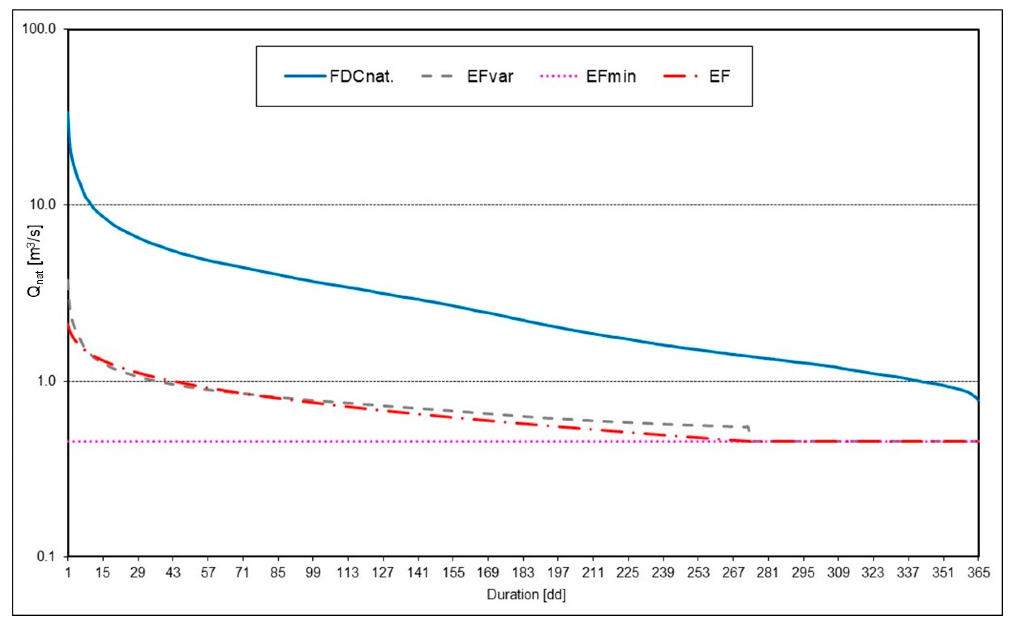
2.1. Water Exploitation Index (WEI+)
2.2. Standardized Precipitation-Evapotranspiration Index (SPEI)
2.3. Spatial Data Interpolation: Kriging Method
2.4. Spatial Data Quantification
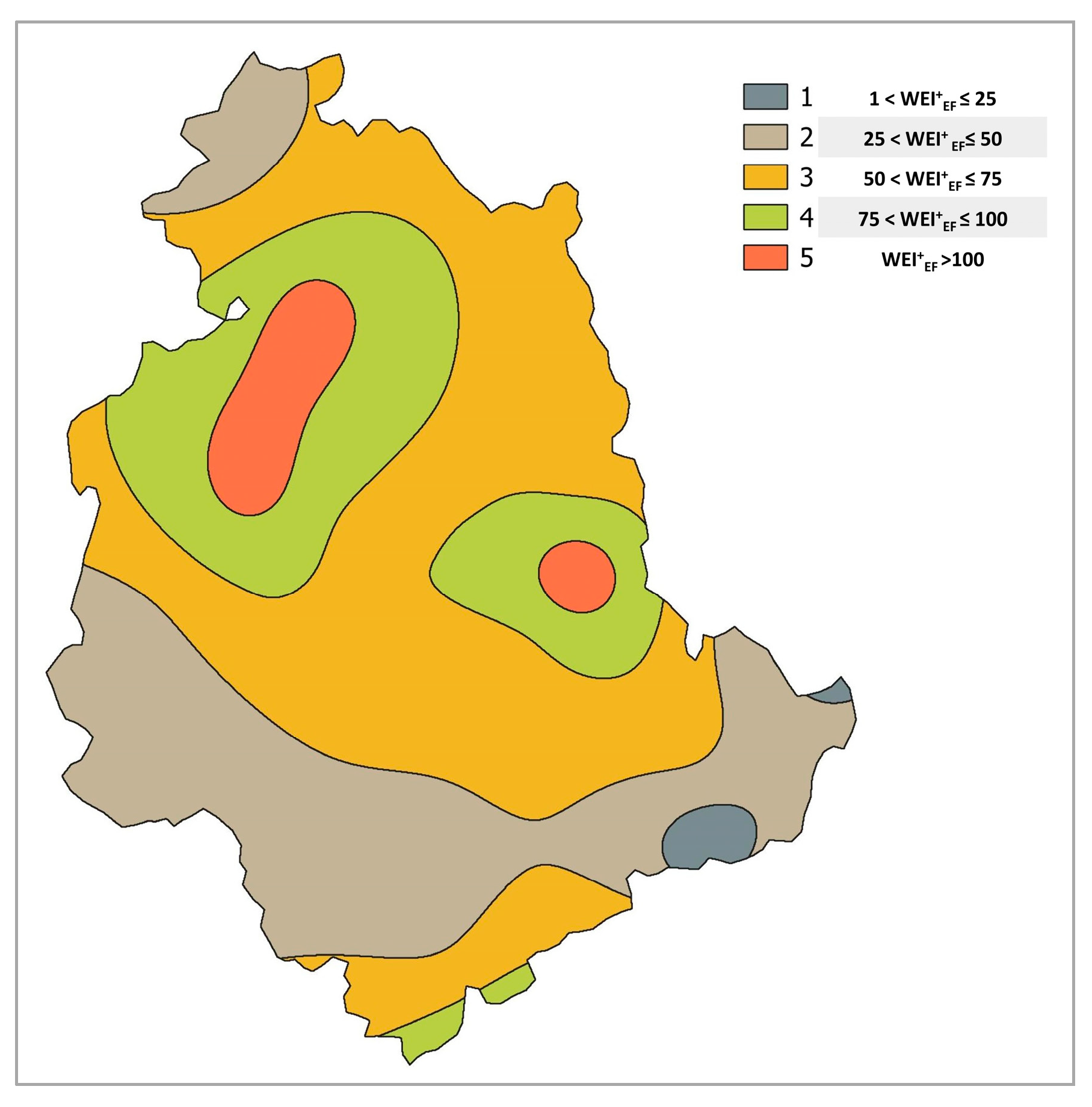
- Both for spatialized values of the WEI+EF and SPEI, within the Umbria region boundary, classes characterized by the same amplitude, with an increasing criticality level, were identified. In particular, five classes were found for the WEI+EF (Table 2) [52], and four classes were found both for the average and 10th percentile values of SPEI 3 sept (Table 3). The four SPEI classes were selected to ensure that the intervals were symmetrically distributed around a specific value. For the average, this value was zero, representing the mean of the normal standard distribution. For the 10th percentile, the value was −1, which was considered the threshold separating normal conditions from moderately dry conditions (Table 1).
- 2.
- 3.
- The QGIS Clip raster by mask layer tool allowed us to clip the raster maps of SPEI 3 using, as a mask, the vector WEI+ zones in Figure 3. In this way, it was possible to identify how many pixels in the SPEI maps were included in the different classes of WEI+EF. As an example, Figure 4 shows the distribution of SPEI 3 sept values (10th percentile) that belong to the 4th class of WEI+EF.
- 4.
- For each WEI+EF class, a specific expression was set in the QGIS Raster Calculator tool, and the SPEI pixels (for both the average and 10th percentile classes) were classified according to the intervals in Table 3.
3. Study Area and Data
4. Results
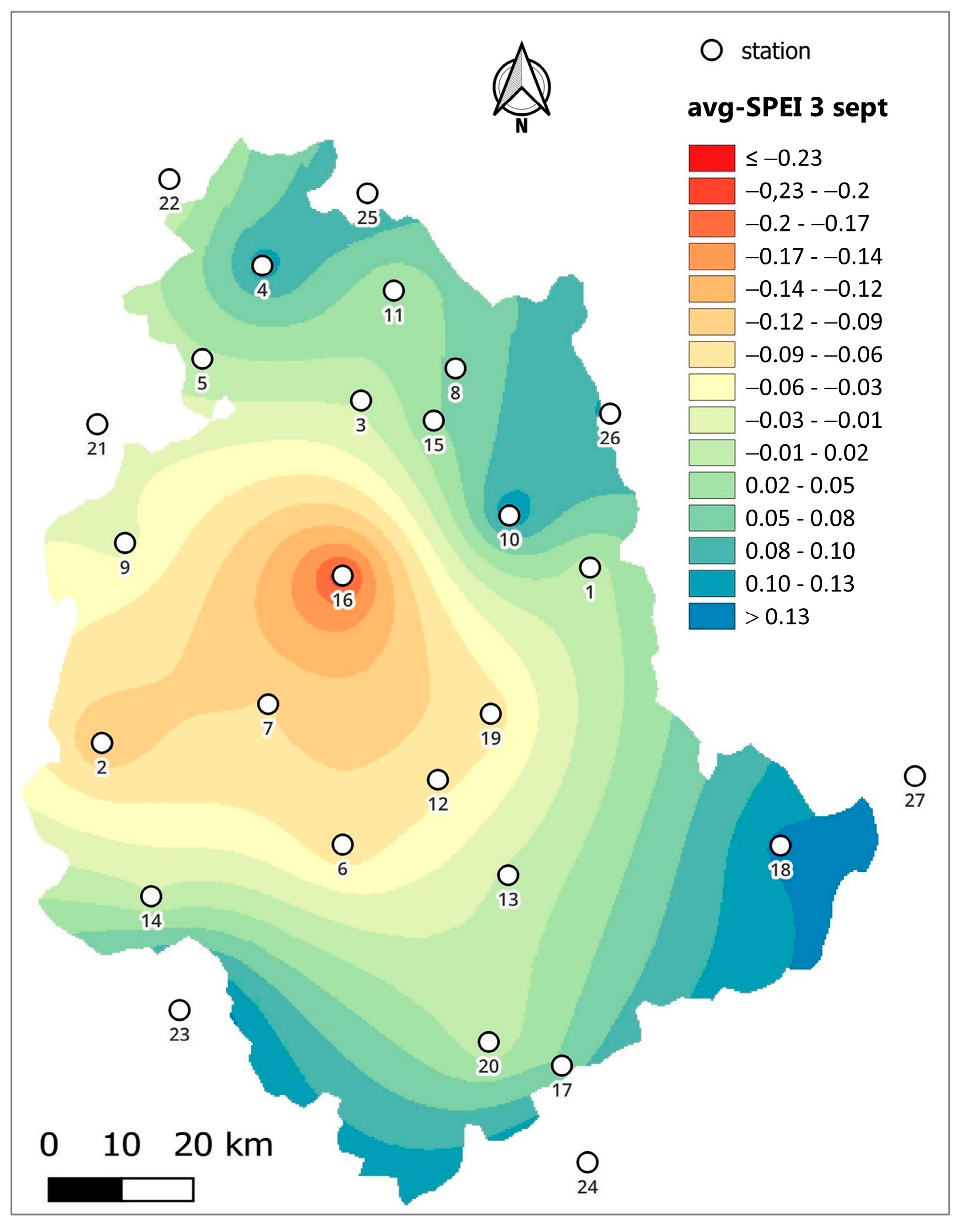
4.1. SPEI 3 Sept Analysis
4.2. WEI+EF Low Flow Analysis
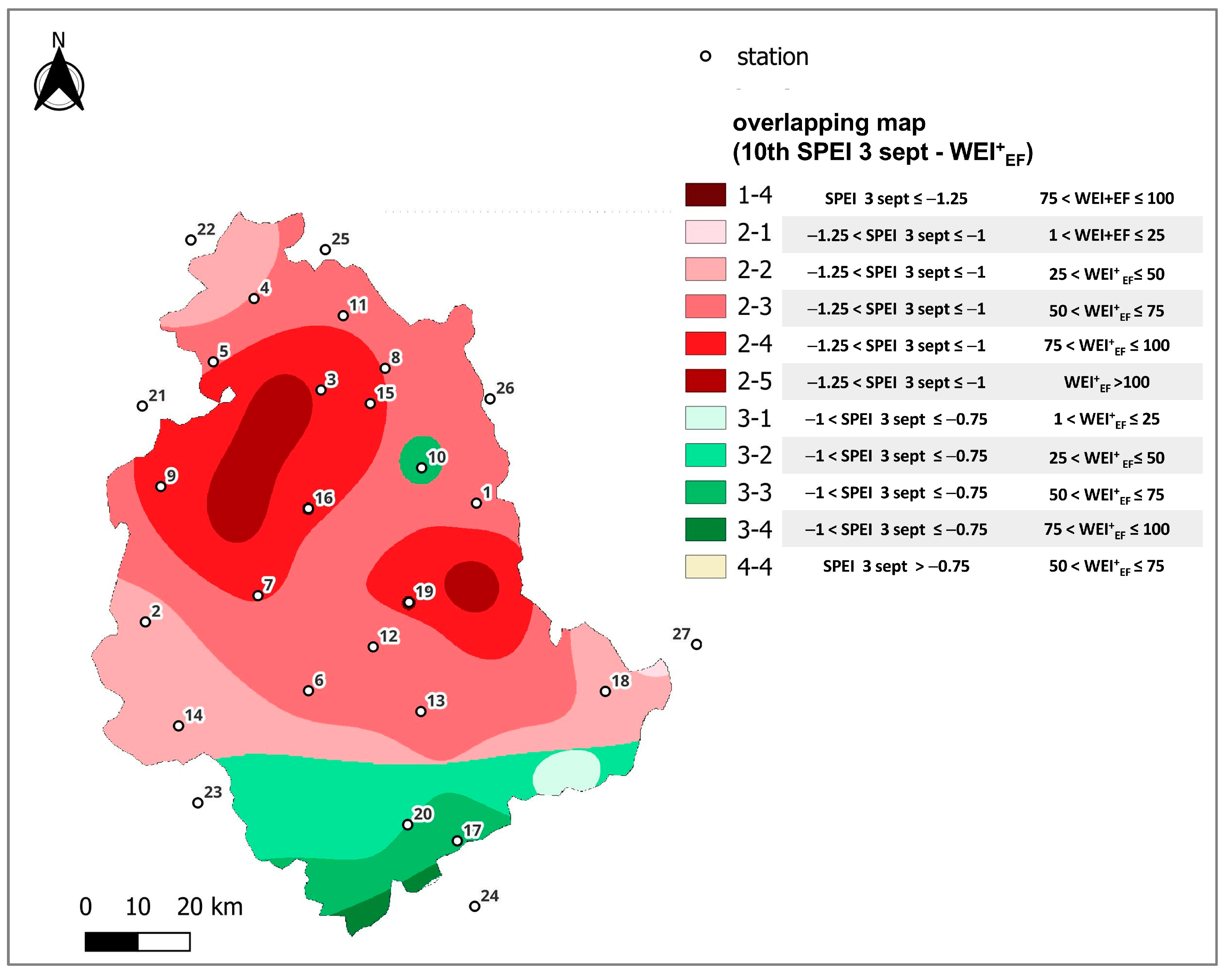
4.3. Results Overlap of SPEI 3 Sept and WEI+EF Low Flow
5. Discussion
6. Conclusions
Supplementary Materials
Author Contributions
Funding
Data Availability Statement
Acknowledgments
Conflicts of Interest
Appendix A

| Annual Cumulative Rainfall (mm) | Temperature (°C) | |||||
|---|---|---|---|---|---|---|
| ID | Name | Mean | Minimum | Maximum | Maximum | Minimum |
| 1 | Nocera Umbra | 955.9 | 589.2 | 1217.6 | 30.5 | −0.3 |
| 2 | Ponte S.Maria | 789.6 | 308.1 | 1089.4 | 32.2 | −1.4 |
| 3 | Montelovesco | 823.2 | 480.0 | 1270.0 | 31.5 | 1.5 |
| 4 | Citta’di Castello | 853.8 | 559.3 | 1127.9 | 33.1 | −0.7 |
| 5 | Petrelle | 907.4 | 599.2 | 1226.7 | 32.5 | −1.1 |
| 6 | Todi | 773.7 | 430.4 | 1078.9 | 33.1 | 0.5 |
| 7 | Compignano | 761.6 | 471.8 | 1086.7 | 33.9 | −0.7 |
| 8 | Gubbio | 968.3 | 608.2 | 1407.6 | 31.6 | −0.3 |
| 9 | Castiglione del Lago | 759.7 | 468.6 | 987.6 | 33.3 | 0.4 |
| 10 | Casa Castalda | 1019.9 | 579.2 | 1463.4 | 28.8 | 0.3 |
| 11 | S.Benedetto Vecchio | 834.9 | 571.8 | 1149.2 | 28.3 | 0.1 |
| 12 | Bastardo | 861.5 | 530.6 | 1272.8 | 31.9 | 0.3 |
| 13 | S.Silvestro | 885.1 | 625.6 | 1202.0 | 32.1 | 0.6 |
| 14 | Orvieto Scalo | 754.2 | 419.0 | 1217.6 | 33.4 | −0.2 |
| 15 | Carestello | 1026.9 | 618.2 | 1593.0 | 29.9 | −0.3 |
| 16 | Perugia | 856.6 | 547.6 | 1283.2 | 32.3 | 1.7 |
| 17 | Piediluco | 992.3 | 620.0 | 1442.4 | 31.0 | −1.5 |
| 18 | Norcia | 786.4 | 467.4 | 1144.0 | 30.8 | −2.7 |
| 19 | Bevagna | 751.4 | 456.0 | 1084.4 | 33.3 | 0.3 |
| 20 | Terni | 822.9 | 517.0 | 1177.4 | 33.3 | 2.1 |
| 21 | Cortona | 775.1 | 377.6 | 1079.2 | 32.3 | 1.3 |
| 22 | Anghiari | 848.9 | 571.8 | 1165.0 | 31.2 | −1.7 |
| 23 | Bagnoregio | 903.1 | 541.4 | 1246.7 | 29.4 | 2.2 |
| 24 | Rieti | 1062.0 | 644.1 | 1363.9 | 32.3 | −1.9 |
| 25 | Apecchio | 1221.3 | 838.2 | 1500.6 | 29.8 | −1.6 |
| 26 | Campodiegoli | 1112.2 | 442.8 | 1746.8 | 30.5 | 0.6 |
| 27 | Montemonaco | 1139.8 | 709.5 | 1470.4 | 27.1 | 0.3 |
| ID | Name | Basin | Region | Elevation (m a.s.l.) | Latitude (N) | Longitude (E) | First Recording Year | SPEI Time Series Length |
|---|---|---|---|---|---|---|---|---|
| 1 | Nocera Umbra | Tiber | Umbria | 530 | 43.1189 | 12.7911 | 1921 (P) 1988 (T) | 2000–2022 |
| 2 | Ponte S.Maria | Tiber | Umbria | 240 | 42.8958 | 12.0214 | 1988 (P) 1989 (T) | 2000–2022 |
| 3 | Montelovesco | Tiber | Umbria | 632 | 43.3069 | 12.4167 | 1921 (P) 1995 (T) | 2000–2022 |
| 4 | Citta’di Castello | Tiber | Umbria | 304 | 43.4614 | 12.2514 | 1951 | 2003–2022 |
| 5 | Petrelle | Tiber | Umbria | 346 | 43.3497 | 12.16 | 1921 (P) 1988 (T) | 2000–2022 |
| 6 | Todi | Tiber | Umbria | 326 | 42.7861 | 12.4092 | 1921 (P) 1934 (T) | 1960–2022 |
| 7 | Compignano | Tiber | Umbria | 238 | 42.9478 | 12.2836 | 1921 (P) 1995 (T) | 2000–2022 |
| 8 | Gubbio | Tiber | Umbria | 471 | 43.3478 | 12.5667 | 1947 | 2000–2022 |
| 9 | Castiglione del Lago | Tiber | Umbria | 259 | 43.1308 | 12.0464 | 1921 (P) 2008 (T) | 2009–2022 |
| 10 | Casa Castalda | Tiber | Umbria | 695 | 43.1775 | 12.6597 | 1992 (P) 1994 (T) | 2000–2022 |
| 11 | S.Benedetto Vecchio | Tiber | Umbria | 729 | 43.4367 | 12.4639 | 1955 (P) 1994 (T) | 2000–2022 |
| 12 | Bastardo | Tiber | Umbria | 331 | 42.8653 | 12.5578 | 1951 (P) 1994 (T) | 2004–2022 |
| 13 | S.Silvestro | Tiber | Umbria | 379 | 42.7558 | 12.6739 | 1992 (P) 1994 (T) | 2000–2022 |
| 14 | Orvieto Scalo | Tiber | Umbria | 311 | 42.718 | 12.1077 | 1921 (P) 1948 (T) | 2000–2022 |
| 15 | Carestello | Tiber | Umbria | 518 | 43.2861 | 12.5342 | 1999 (P) 1994 (T) | 2000–2022 |
| 16 | Perugia | Tiber | Umbria | 437 | 43.1012 | 12.3959 | 1924 | 1960–2022 |
| 17 | Piediluco | Tiber | Umbria | 369 | 42.5342 | 12.7672 | 1996 | 2000–2022 |
| 18 | Norcia | Tiber | Umbria | 690 | 42.7986 | 13.105 | 1951 | 2004–2022 |
| 19 | Bevagna | Tiber | Umbria | 211 | 42.9442 | 12.6389 | 1921 (P) 1998 (T) | 2004–2022 |
| 20 | Terni | Tiber | Umbria | 122 | 42.5597 | 12.6503 | 1921 (P) 1947 (T) | 1960–2022 |
| 21 | Cortona | Arno | Tuscany | 413 | 43.269 | 11.996 | 1991 (P) 2000 (T) | 2000–2022 |
| 22 | Anghiari | Tiber | Tuscany | 314 | 43.559 | 12.097 | 2012 (P) 1993 (T) | 2000–2022 |
| 23 | Bagnoregio | Tiber | Lazio | 361 | 42.586 | 12.1588 | 1997 | 2004–2022 |
| 24 | Rieti | Tiber | Lazio | 377 | 42.4218 | 12.8118 | 1986 | 2007–2022 |
| 25 | Apecchio | Metauro | Marche | 544 | 43.55 | 12.4167 | 2003 | 2007–2022 |
| 26 | Campodiegoli | Esino | Marche | 559 | 43.3 | 12.8167 | 2001 (P) 2003 (T) | 2007–2022 |
| 27 | Montemonaco | Aso | Marche | 987 | 42.8833 | 13.3167 | 2003 | 2007–2022 |
| Drainage Basin Centroid | River | Basin Area (Km2) | Gauged Station | Name | Latitude (N) | Longitude (E) | FDCs Time Series |
|---|---|---|---|---|---|---|---|
| 1 | Tiber | 363.55 | No | ||||
| 2 | Tiber | 4145.00 | Yes | Ponte Nuovo | 43.0103 | 12.4292 | 1994–2021 |
| 3 | Tiber | 5748.17 | No | ||||
| 4 | Tiber | 928.92 | Yes | Santa Lucia | 43.4217 | 12.2389 | 1991–2021 |
| 5 | Tiber | 2191.00 | No | ||||
| 6 | Chiascio | 481.00 | No | ||||
| 7 | Chiascio | 538.00 | Yes | Pianello | 43.1439 | 12.5653 | 1998–2021 |
| 8 | Chiascio | 1956.00 | Yes | Ponte Rosciano | 43.0250 | 12.4456 | 1997–2022 |
| 9 | Topino | 191.00 | Yes | Valtopina | 43.0533 | 12.7558 | 1997–2021 |
| 10 | Topino | 446.20 | No | ||||
| 11 | Topino | 1094.33 | Yes | Cannara | 42.9958 | 12.5842 | 1994–2021 |
| 12 | Topino | 1215.00 | Yes | Bettona | 43.0247 | 12.5097 | 1994–2021 |
| 13 | Marroggia | 65.00 | Yes | Azzano | 42.8125 | 12.7569 | 1994–2022 |
| 14 | Timia | 608.40 | No | ||||
| 15 | Nestore | 447.20 | Yes | Mercatello | 42.9742 | 12.2664 | 2005–2022 |
| 16 | Nestore | 705.71 | Yes | Marsciano | 42.9161 | 12.3372 | 1991–2021 |
| 17 | Paglia | 802.60 | No | ||||
| 18 | Paglia | 1285.40 | Yes | Orvieto Scalo | 42.7244 | 12.1358 | 1992–2021 |
| 19 | Paglia | 1357.70 | No | ||||
| 20 | Corno | 438.76 | No | ||||
| 21 | Nera | 144.5 | No | ||||
| 22 | Nera | 1362.11 | Yes | Torreorsina | 42,5717 | 12.7403 | 1997–2021 |
| 23 | Nera | 3881.88 | No | ||||
| 24 | Nera | 4308.80 | No |
Appendix B
| Monitoring Station | 2012 | 2013 | 2014 | 2015 | 2016 | 2017 | 2018 | 2019 | 2020 | 2021 | 2022 |
|---|---|---|---|---|---|---|---|---|---|---|---|
| Nocera Umbra | −0.408 | −2.289 | 1.807 | −0.238 | 0.397 | −0.552 | −0.768 | 0.685 | 0.800 | −1.377 | 1.375 |
| Ponte S.Maria | −1.214 | 0.079 | 0.544 | −0.927 | 0.128 | −1.693 | −0.529 | 0.323 | 0.820 | −1.277 | 1.362 |
| Montelovesco | −0.795 | 1.200 | 1.313 | −1.475 | −0.383 | −1.071 | −0.414 | 0.667 | 0.190 | −0.677 | 1.180 |
| Citta’di Castello | −0.298 | −0.190 | 1.537 | −0.853 | 0.038 | 0.400 | −1.351 | 1.370 | 0.882 | −0.557 | 1.749 |
| Petrelle | −0.433 | 0.657 | 0.868 | −2.090 | −0.222 | −0.931 | −0.568 | 0.834 | 0.609 | −0.494 | 2.018 |
| Todi | −0.622 | −0.128 | 0.860 | −0.270 | 0.147 | 0.355 | −1.144 | −0.211 | 0.745 | −2.122 | 0.546 |
| Compignano | 0.247 | −0.850 | 1.794 | −0.378 | 0.448 | −0.653 | −0.585 | −0.164 | 0.982 | −2.165 | 0.202 |
| Gubbio | −1.880 | 1.082 | 1.542 | −0.949 | 0.310 | −0.860 | −0.791 | 0.403 | 0.543 | −0.144 | 1.484 |
| Castiglione del Lago | −1.371 | 0.522 | 1.570 | −0.420 | 0.467 | −0.838 | −1.140 | −0.279 | 1.100 | −0.963 | 1.357 |
| Casa Castalda | 0.056 | −0.289 | 1.532 | −1.166 | 0.553 | −0.413 | −0.482 | 0.308 | 1.902 | 0.014 | 1.181 |
| S.Benedetto Vecchio | −0.656 | −0.009 | 1.695 | −1.144 | 0.140 | −1.961 | −0.938 | 0.555 | 0.449 | −0.229 | 1.665 |
| Bastardo | −1.016 | −0.016 | 0.878 | −1.211 | 1.048 | −0.416 | −1.339 | −0.074 | 1.418 | −1.608 | 1.155 |
| S.Silvestro | −1.422 | 0.972 | 1.162 | 0.536 | −0.287 | −0.706 | −0.604 | 0.093 | 0.819 | −1.723 | 1.133 |
| Orvieto Scalo | −1.312 | −0.197 | 1.359 | −0.629 | 0.000 | 0.205 | 0.253 | −0.123 | 0.886 | −2.141 | 1.268 |
| Carestello | −1.678 | 0.939 | 1.115 | −1.142 | 0.079 | −0.454 | −0.962 | 0.438 | 1.923 | −0.760 | 1.258 |
| Perugia Fontivegge | −1.336 | −0.152 | 0.961 | −1.574 | −0.461 | −1.372 | −1.665 | −0.108 | 0.581 | −1.072 | 1.198 |
| Piediluco | −0.675 | 1.230 | 1.166 | −0.016 | −0.164 | −0.240 | 0.195 | −0.238 | −0.425 | −1.568 | 0.987 |
| Norcia | 0.253 | 0.822 | 1.486 | 0.851 | 0.189 | −0.025 | −1.151 | 0.450 | −0.619 | −1.136 | 1.145 |
| Bevagna | −0.577 | −1.494 | 1.497 | −0.412 | −0.165 | 0.961 | −1.692 | −0.672 | 1.083 | −0.919 | 0.729 |
| Terni | −0.612 | 0.608 | 0.195 | −0.160 | 0.125 | −0.061 | −0.288 | 0.359 | −0.057 | −1.530 | 0.544 |
| Cortona | 0.233 | −0.738 | 1.388 | −0.897 | 0.919 | −0.738 | −1.073 | 0.246 | 0.630 | −1.500 | 1.011 |
| Anghiari | −0.612 | 0.337 | 1.548 | −0.910 | −0.617 | −0.279 | −1.529 | 0.437 | 0.804 | −1.953 | 1.724 |
| Bagnoregio | 0.490 | 0.800 | 1.554 | 1.537 | 0.912 | −0.959 | −0.629 | 0.506 | −0.294 | −0.284 | 1.044 |
| Rieti | 0.505 | 0.434 | 0.312 | −0.182 | 0.732 | −0.569 | 0.871 | −0.277 | −0.335 | 0.225 | 2.100 |
| Apecchio | −0.118 | −0.013 | 1.653 | −0.148 | 0.408 | 0.055 | −1.105 | 0.641 | 0.207 | −1.239 | 1.755 |
| Campodiegoli | 0.117 | −0.119 | 1.718 | 0.029 | −0.542 | −1.051 | −1.511 | 0.401 | 1.211 | −0.020 | 1.451 |
| Montemonaco | 1.637 | 0.339 | 0.590 | −0.317 | 1.032 | −0.698 | 1.389 | 1.290 | −1.369 | −1.058 | −0.967 |
References
- WWAP (United Nations World Water Assessment Programme). Water for a Sustainable World. In The United Nations World Water Development Report 2015; UNESCO: Paris, France, 2015. [Google Scholar]
- Veloso, S.; Tam, C.; Oliveira, T. Effects of extreme drought and water scarcity on consumer behaviour—The impact of water consumption awareness and Consumers’ choices. J. Hydrol. 2024, 639, 131574. [Google Scholar] [CrossRef]
- Di Francesco, S.; Venturi, S.; Casadei, S. An integrated water resource management approach for Lake Trasimeno, Italy. Hydrol. Sci. J. 2023, 68, 630–644. [Google Scholar] [CrossRef]
- Bertoli, L.; Balzarolo, D.; Todini, E. On the Benefits of Collaboration between Decision Makers and Scientists: The Case of Lake Como. Hydrology 2022, 9, 187. [Google Scholar] [CrossRef]
- Song, Y.; Joo, J.; Kim, H.; Park, M. Development and Applicability Evaluation of Damage Scale Analysis Techniques for Agricultural Drought. Water 2024, 16, 1342. [Google Scholar] [CrossRef]
- Masip Macía, Y.; Nuñez González, S.M.; Villazon Carmona, E.J.; Burgos Pezoa, M. Bibliometric Analysis of Renewable Energy Strategies for Mitigating the Impact of Severe Droughts on Electrical Systems. Appl. Sci. 2025, 15, 2060. [Google Scholar] [CrossRef]
- Stubbington, R.; England, J.; Sarremejane, R.; Watts, G.; Wood, P.J. The effects of drought on biodiversity in UK river ecosystems: Drying rivers in a wet country. WIREs Water 2024, 11, e1745. [Google Scholar] [CrossRef]
- Napoli, A.; Matiu, M.; Laiti, L.; Barbiero, R.; Bellin, A.; Zardi, D.; Majone, B. Review on climate change impacts on the Water-Energy-Food-Ecosystems (WEFE) Nexus in the North-Eastern Italian Alps. Clim. Change 2025, 178, 41. [Google Scholar] [CrossRef]
- Gu, L.; Chen, J.; Yin, J.; Sullivan, S.C.; Wang, H.-M.; Guo, S.; Zhang, L.; Kim, J.-S. Projected increases in magnitude and socioeconomic exposure of global droughts in 1.5 and 2 °C warmer climates. Hydrol. Earth Syst. Sci. 2020, 24, 451–472. [Google Scholar] [CrossRef]
- Lorenzo, M.N.; Pereira, H.; Alvarez, I.; Dias, J.M. Standardized Precipitation Index (SPI) evolution over the Iberian Peninsula during the 21st century. Atmos. Res. 2024, 297, 107132. [Google Scholar] [CrossRef]
- Wang, Q.; Zhang, R.; Qi, J.; Zeng, J.; Wu, J.; Shui, W.; Wu, X.; Li, J. An improved daily standardized precipitation index dataset for mainland China from 1961 to 2018. Sci Data 2022, 9, 124. [Google Scholar] [CrossRef]
- Majd, N.R.; Montaseri, M.; Amirataee, B. Stochastic evaluation of the effect of cross-correlation between rainfall and evapotranspiration on SPEI performance. J. Hydrol. 2025, 652, 132650. [Google Scholar] [CrossRef]
- Zhang, R.; Bento, V.A.; Qi, J.; Xu, F.; Wu, J.; Qiu, J.; Li, J.; Shui, W.; Wang, Q. The first high spatial resolution multi-scale daily SPI and SPEI raster dataset for drought monitoring and evaluating over China from 1979 to 2018. Big Earth Data 2023, 7, 860–885. [Google Scholar] [CrossRef]
- Venturi, S.; Mateescu, E.; Virsta, A.; Petrescu, N.; Dunea, D.; Casadei, S. Drought monitoring in Southeastern Romania based on the comparison and correlation of SPEI and SPI indices. Sci. Pap. Ser. E Land Reclam. Earth Obs. Surv. Environ. Eng. 2024, 13, 655–661. [Google Scholar]
- Wang, Z.; Yang, Y.; Zhang, C.; Guo, H.; Hou, Y. Historical and future Palmer Drought Severity Index with improved hydrological modeling. J. Hydrol. 2022, 610, 127941. [Google Scholar] [CrossRef]
- Zhou, Y.; Zhou, P.; Jin, J.; Wu, C.; Cui, Y.; Zhang, Y.; Tong, F. Drought identification based on Palmer drought severity index and return period analysis of drought characteristics in Huaibei Plain China. Environ. Res. 2022, 212, 113163. [Google Scholar] [CrossRef]
- Gonçalves, S.T.N.; Vasconcelos Júnior, F.d.C.; Silveira, C.d.S.; Cid, D.A.C.; Martins, E.S.P.R.; Costa, J.M.F.d. Comparative Analysis of Drought Indices in Hydrological Monitoring in Ceará’s Semi-Arid Basins, Brazil. Water 2023, 15, 1259. [Google Scholar] [CrossRef]
- Khoshnazar, A.; Corzo Perez, G.A.; Diaz, V.; Aminzadeh, M.; Cerón Pinedad, R.A. Wet-environment Evapotranspiration and Precipitation Standardized Index (WEPSI) for drought assessment and monitoring. Hydrol. Res. 2022, 53, 1393–1413. [Google Scholar] [CrossRef]
- Venturi, S.; Dunea, D.; Mateescu, E.; Virsta, A.; Petrescu, N.; Casadei, S. SPEI and SPI correlation in the study of drought phenomena in Umbria region (central Italy). Environ. Sci. Pollut. Res. 2024, 32, 168–188. [Google Scholar] [CrossRef]
- Vergni, L.; Dari, J.; Todisco, F.; Vizzari, M.; Saltalippi, C.; Venturi, S.; Casadei, S.; Brocca, L. Quantifying Irrigation Volumes Using Sentinel-1 Soil Moisture Data in Central Italy. In AIIA 2022: Biosystems Engineering Towards the Green Deal; Ferro, V., Giordano, G., Orlando, S., Vallone, M., Cascone, G., Porto, S.M.C., Eds.; Lecture Notes in Civil Engineering; Springer: Cham, Switzerland, 2023; Volume 337. [Google Scholar] [CrossRef]
- Leijnse, M.; Bierkens, M.F.P.; Gommans, K.H.M.; Lin, D.; Tait, A.; Wanders, N. Key drivers and pressures of global water scarcity hotspots. Environ. Res. Lett. 2024, 19, 5. [Google Scholar] [CrossRef]
- Russo, A.; Gouveia, C.M.; Dutra, E.; Soares, P.M.M.; Trigo, R.M. The synergy between drought and extremely hot summers in the Mediterranean. Environ. Res. Lett. 2019, 14, 1. [Google Scholar] [CrossRef]
- Avino, A.; Cimorelli, L.; Furcolo, P.; Noto, L.V.; Pelosi, A.; Pianese, D.; Villani, P.; Manfreda, S. Are rainfall extremes increasing in southern Italy? J. Hydrol. 2024, 631, 130684. [Google Scholar] [CrossRef]
- Romano, E.; Petrangeli, A.B.; Salerno, F.; Guyennon, N. Do recent meteorological drought events in central Italy result from long-term trend or increasing variability? Int. J. Climatol. 2022, 42, 4111–4128. [Google Scholar] [CrossRef]
- Pronti, A.; Auci, S.; Mazzanti, M. Adopting sustainable irrigation technologies in Italy: A study on the determinants of inter- and intra-farm diffusion. Econ. Innov. New Technol. 2023, 33, 299–322. [Google Scholar] [CrossRef]
- Masseroni, D.; Gangi, F.; Ghilardelli, F.; Gallo, A.; Kisekka, I.; Gandolfi, C. Assessing the water conservation potential of optimized surface irrigation management in Northern Italy. Irrig Sci. 2024, 42, 75–97. [Google Scholar] [CrossRef]
- Casadei, S.; Di Francesco, S.; Giannone, F.; Pierleoni, A. Small reservoirs for a sustainable water resources management. Adv. Geosci. (ADGEO) 2019, 49, 165–174. [Google Scholar] [CrossRef]
- Di Francesco, S.; Casadei, S.; Di Mella, I.; Giannone, F. The role of small reservoirs in a water scarcity scenario: A computational approach. Water Resour. Manag. 2022, 36, 875–889. [Google Scholar] [CrossRef]
- Fan, L.; Wang, H.; Liu, Z.; Li, N. Quantifying the Relationship between Drought and Water Scarcity Using Copulas: Case Study of Beijing–Tianjin–Hebei Metropolitan Areas in China. Water 2018, 10, 1622. [Google Scholar] [CrossRef]
- Faergemann, H. Update on Water Scarcity and Droughts indicator development. In EC Expert Group on Water Scarcity & Droughts; European Environment Agency: Brussels, Belgium, 2012; pp. 1–23. [Google Scholar]
- Gumus, V.; Algin, H.M. Meteorological and hydrological drought analysis of the Seyhan−Ceyhan River Basins, Turkey. Met. Apps. 2017, 24, 62–73. [Google Scholar] [CrossRef]
- Morbidelli, R.; Saltalippi, C.; Flammini, A.; Dari, J.; Venturi, S.; Casadei, S. Principali Indicatori Climatici in Umbria—Rapporto 2023. Cent. Interuniv. Per L’Ambiente CIPLA; Università di Perugia, 2023. Available online: https://servizioidrografico.regione.umbria.it/pubblicazione/principali-indicatori-climatici-in-umbria-rapporoto-2023/ (accessed on 26 March 2025). (In Italian).
- Bongioannini Cerlini, P.; Saraceni, M.; Silvestri, L.; Meniconi, S.; Brunone, B. Monitoring the Water Mass Balance Variability of Small Shallow Lakes by an ERA5-Land Reanalysis and Water Level Measurement-Based Model. An Application to the Trasimeno Lake, Italy. Atmosphere 2022, 13, 949. [Google Scholar] [CrossRef]
- Casadei, S.; Pierleoni, A.; Bellezza, M. Sustainability of Water Withdrawals in the Tiber River Basin (Central Italy). Sustainability 2018, 10, 485. [Google Scholar] [CrossRef]
- Casadei, S.; Peppoloni, F.; Pierleoni, A. A New Approach to Calculate the Water Exploitation Index (WEI+). Water 2020, 12, 3227. [Google Scholar] [CrossRef]
- Dimkić, D.; Simić, Z. WEI+ as an Indicator of Water Scarcity and Ecological Demand Issue. Water Resour. Manag. 2024, 38, 5759–5781. [Google Scholar] [CrossRef]
- European Commission. Ecological flow in the implementation of the Water Framework Directive. In CIS Guidance Document nº31; EC Publication Office: Luxembourg, 2015. [Google Scholar]
- Schmutz, S.; Bakken, T.H.; Friedrich, T.; Greimle, F.; Harby, A.; Melcher, A.; Jungwirth, M.; Unfer, G.; Zeiringer, B. Response of fish communities to hydrological and morphological alterations in hydropeaking rivers in Austria. River Res. Applic. 2015, 31, 919–930. [Google Scholar] [CrossRef]
- Santos, J.M.; Leite, R.; Costa, M.J.; Godinho, F.; Portela, M.M.; Pinheiro, A.N.; Boavida, I. Seasonal and Size-Related Fish Microhabitat Use Upstream and Downstream from Small Hydropower Plants. Water 2024, 16, 37. [Google Scholar] [CrossRef]
- Tennant, D.L. Instream Flow Regimens for Fish, Wildlife, Recreation and Related Environmental Resources. Fisheries 1976, 1, 6–10. [Google Scholar] [CrossRef]
- Moccia, D.; Salvadori, L.; Ferrari, S.; Carucci, A.; Pusceddu, A. Implementation of the EU ecological flow policy in Italy with a focus on Sardinia. Adv. Oceanogr. Limnol. 2020, 11, 22–34. [Google Scholar] [CrossRef]
- Vicente-Serrano, S.M.; Beguería, S.; López-Moreno, J.I. A multiscalar drought index sensitive to global warming: The standardized precipitation evapotranspiration index. J. Clim. 2010, 23, 1696–1718. [Google Scholar] [CrossRef]
- Herold, N.; Ekström, M.; Kala, J.; Goldie, J.; Evans, J.P. Australian climate extremes in the 21st century according to a regional climate model ensemble: Implications for health and agriculture. Weather. Clim. Extrem. 2018, 20, 54–68. [Google Scholar] [CrossRef]
- Svoboda, M.; Hayes, M.; Wood, D. Standardized Precipitation Index User Guide; World Meteorological Organization: Geneva, Switzerland, 2012. [Google Scholar]
- Hargreaves, G.H.; Allen, R.G. History and evaluation of Hargreaves evapotranspiration equation. J. Irrigat. Drain. Eng. 2003, 129, 53–63. [Google Scholar] [CrossRef]
- Beguería, S.; Vicente-Serrano, S.M.; Reig, F.; Latorre, B. Standardized precipitation evapotranspiration index (SPEI) revisited: Parameter fitting, evapotranspiration models, tools, datasets and drought monitoring. Int. J. Climatol. 2014, 34, 3001–3023. [Google Scholar] [CrossRef]
- Abramowitz, M.; Stegun, I.A. Handbook of Mathematical Functions, with Formulas, Graphs, and Mathematical Tables; Dover Publications: New York, NY, USA, 1965; p. 1046. [Google Scholar]
- Migliaccio, F.; Carrion, D. Sistemi Informativi Territoriali Principi e Applicazioni, 2nd ed.; UTET, De Agostini Scuola SpA: Novara, Italy, 2020. [Google Scholar]
- Oliver, M.; Webster, R. Basics Steps in Geostatistics: The Variogram and Kriging. Springer Briefs in Agriculture; Springer: Cham, Switzerland; Heidelberg, Germany; New York, NY, USA, 2015. [Google Scholar] [CrossRef]
- Gribov, A.; Krivoruchko, K. Empirical Bayesian kriging implementation and usage. Sci. Total Environ. 2020, 722, 137290. [Google Scholar] [CrossRef]
- Pilz, J.; Spöck, G. Why do we need and how should we implement Bayesian kriging methods. Stoch. Environ. Res. Risk Assess. 2008, 22, 621–632. [Google Scholar] [CrossRef]
- Estrela-Segrelles, C.; Pérez-Martín, M.Á.; Wang, Q.J. Adapting Water Resources Management to Climate Change in Water-Stressed River Basins—Júcar River Basin Case. Water 2024, 16, 1004. [Google Scholar] [CrossRef]
- Wackernagel, H. The Smoothness of Kriging. In Multivariate Geostatistics; Springer: Berlin/Heidelberg, Germany, 2003. [Google Scholar] [CrossRef]
- Sutanto, S.J.; Duku, C.; Gülveren, M.; Dankers, R.; Paparrizos, S. Future intensification of compound and cascading drought and heatwave risks in Europe. EGUsphere 2025. [Google Scholar] [CrossRef]
- European Environment Agency. Water Exploitation Index Plus (WEI+) for River Basin Districts (1990–2015) GIS Map Application Published 10 October 2018 Last Modified 28 November 2019. Available online: https://www.eea.europa.eu/data-and-maps/explore-interactive-maps/water-exploitation-index-for-river-2 (accessed on 9 March 2025).


| SPEI Value Intervals | SPEI Class |
|---|---|
| SPEI ≥ 2 | Extremely wet |
| 2 > SPEI ≥ 1.5 | Severely wet |
| 1.5 > SPEI ≥ 1 | Moderately wet |
| 1 > SPEI > −1 | Normal |
| −1 ≥ SPEI > −1.5 | Moderately dry |
| −1.5 ≥ SPEI > −2 | Severely dry |
| SPEI ≤ −2 | Extremely dry |
| Classes | WEI+EF Values Intervals |
|---|---|
| 1 | 1 < WEI+EF ≤ 25 |
| 2 | 25 < WEI+ EF ≤ 50 |
| 3 | 50 < WEI+EF ≤ 75 |
| 4 | 75 < WEI+EF ≤ 100 |
| 5 | WEI+EF > 100 |
| Classes | Average | 10th Percentile |
|---|---|---|
| 1 | SPEI ≤ −0.2 | SPEI ≤ −1.25 |
| 2 | −0.2 < SPEI ≤ 0 | −1.25 < SPEI ≤ −1 |
| 3 | 0 < SPEI ≤ 0.2 | −1 < SPEI ≤ −0.75 |
| 4 | SPEI > 0.2 | SPEI > −0.75 |
| Station | Average | 10th Percentile | Station | Average | 10th Percentile |
|---|---|---|---|---|---|
| Nocera Umbra | −0.052 | −1.377 | Carestello | 0.069 | −1.142 |
| Ponte S.Maria | −0.217 | −1.277 | Perugia | −0.454 | −1.574 |
| Montelovesco | −0.024 | −1.071 | Piediluco | 0.023 | −0.675 |
| Citta’di Castello | 0.248 | −0.853 | Norcia | 0.206 | −1.136 |
| Petrelle | 0.022 | −0.931 | Bevagna | −0.151 | −1.494 |
| Todi | −0.168 | −1.144 | Terni | −0.080 | −0.612 |
| Compignano | −0.102 | −0.850 | Cortona | −0.047 | −1.073 |
| Gubbio | 0.068 | −0.949 | Anghiari | −0.095 | −1.529 |
| Castiglione del Lago | 0.000 | −1.140 | Bagnoregio | 0.425 | −0.629 |
| Casa Castalda | 0.291 | −0.482 | Rieti | 0.347 | −0.335 |
| S.Benedetto Vecchio | −0.039 | −1.144 | Apecchio | 0.190 | −1.105 |
| Bastardo | −0.107 | −1.339 | Campodiegoli | 0.153 | −1.051 |
| S.Silvestro | −0.002 | −1.422 | Montemonaco | 0.170 | −1.058 |
| Orvieto Scalo | −0.039 | −1.312 |
| ID Drainage Basin | WEI+EF [%] | ID Drainage Basin | WEI+EF [%] | ID Drainage Basin | WEI+EF [%] |
|---|---|---|---|---|---|
| 1 | 2353 | 9 | 59 | 17 | 32 |
| 2 | 62 | 10 | 121 | 18 | 33 |
| 3 | 61 | 11 | 77 | 19 | 36 |
| 4 | 25 | 12 | 81 | 20 | 1 |
| 5 | 111 | 13 | 58 | 21 | 14 |
| 6 | 65 | 14 | 60 | 22 | 65 |
| 7 | 68 | 15 | 112 | 23 | 261 |
| 8 | 64 | 16 | 78 | 24 | 40 |
| Class | 1 < WEI+EF ≤ 25 (%) | 25 < WEI+EF ≤ 50 (%) | 50 < WEI+EF ≤ 75 (%) | 75 < WEI+EF ≤ 100 (%) | WEI+EF ≥ 100 (%) | |
|---|---|---|---|---|---|---|
| 1 | avg-SPEI 3 sept ≤ −0.2 | 0.00 | 0.00 | 0.00 | 0.30 | 0.00 |
| 2 | −0.2 < avg-SPEI 3 sept ≤ 0 | 0.00 | 28.03 | 42.54 | 63.94 | 89.19 |
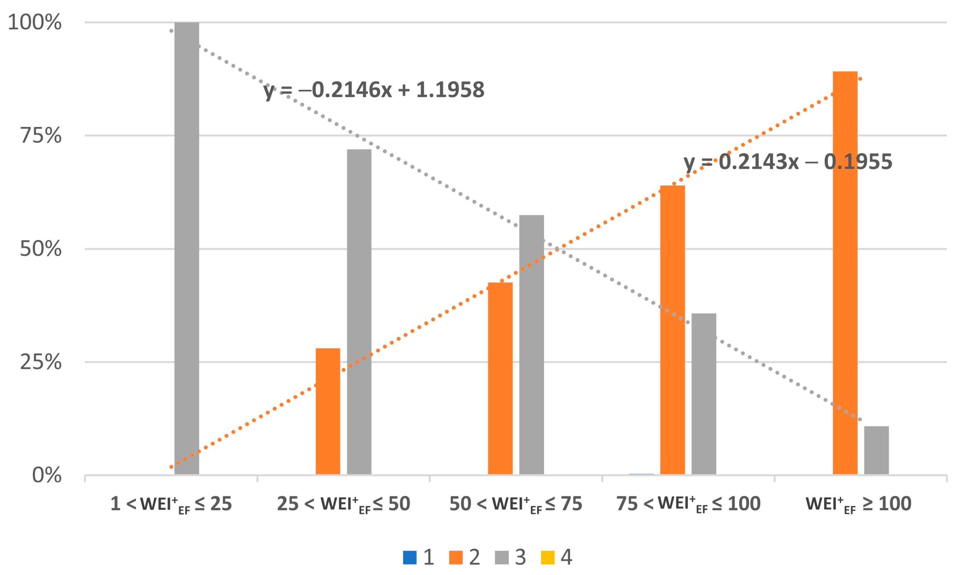
| 3 | 0 < avg-SPEI 3 sept ≤ 0.2 | 100.00 | 71.97 | 57.46 | 35.76 | 10.81 |
| 4 | avg-SPEI 3 sept > 0.2 | 0.00 | 0.00 | 0.00 | 0.00 | 0.00 |
| Class | 1 < WEI+EF ≤ 25 (%) | 25 < WEI+EF ≤ 50 (%) | 50 < WEI+EF ≤ 75 (%) | 75 < WEI+EF ≤ 100 (%) | WEI+EF ≥ 100 (%) | |
|---|---|---|---|---|---|---|
| 1 | SPEI 3 sept ≤ −1.25 | 0.00 | 0.00 | 0.00 | 0.57 | 0.00 |
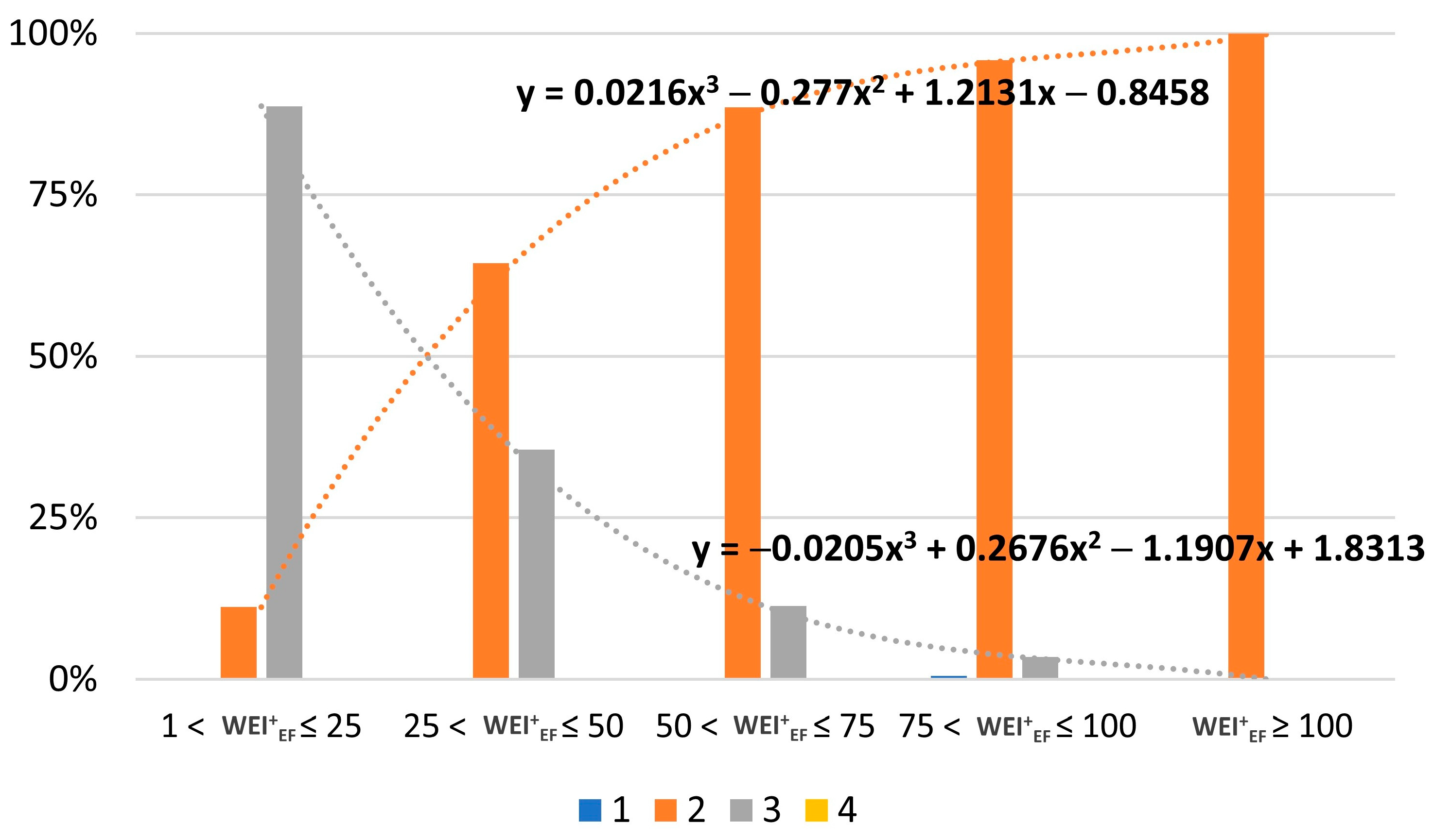
| 2 | −1.25 < SPEI 3 sept ≤ −1 | 11.22 | 64.47 | 88.62 | 95.87 | 100.00 |
| 3 | −1 < SPEI 3 sept ≤ −0.75 | 88.78 | 35.53 | 11.38 | 3.47 | 0.00 |
| 4 | SPEI 3 sept > −0.75 | 0.00 | 0.00 | 0.00 | 0.09 | 0.00 |
Disclaimer/Publisher’s Note: The statements, opinions and data contained in all publications are solely those of the individual author(s) and contributor(s) and not of MDPI and/or the editor(s). MDPI and/or the editor(s) disclaim responsibility for any injury to people or property resulting from any ideas, methods, instructions or products referred to in the content. |
© 2025 by the authors. Licensee MDPI, Basel, Switzerland. This article is an open access article distributed under the terms and conditions of the Creative Commons Attribution (CC BY) license (https://creativecommons.org/licenses/by/4.0/).
Share and Cite
Casadei, S.; Venturi, S.; Di Francesco, S. Comparative Analysis of SPEI and WEI+ Indices: Drought and Water Scarcity in the Umbria Region, Central Italy. Hydrology 2025, 12, 74. https://doi.org/10.3390/hydrology12040074
Casadei S, Venturi S, Di Francesco S. Comparative Analysis of SPEI and WEI+ Indices: Drought and Water Scarcity in the Umbria Region, Central Italy. Hydrology. 2025; 12(4):74. https://doi.org/10.3390/hydrology12040074
Chicago/Turabian StyleCasadei, Stefano, Sara Venturi, and Silvia Di Francesco. 2025. "Comparative Analysis of SPEI and WEI+ Indices: Drought and Water Scarcity in the Umbria Region, Central Italy" Hydrology 12, no. 4: 74. https://doi.org/10.3390/hydrology12040074
APA StyleCasadei, S., Venturi, S., & Di Francesco, S. (2025). Comparative Analysis of SPEI and WEI+ Indices: Drought and Water Scarcity in the Umbria Region, Central Italy. Hydrology, 12(4), 74. https://doi.org/10.3390/hydrology12040074