Predicting Water Distribution and Optimizing Irrigation Management in Turfgrass Rootzones Using HYDRUS-2D

Abstract

The increasing global reliance on water resources has necessitated improvements in turfgrass irrigation efficiency. This study aimed to compare measured field data with predicted data on irrigation water distribution in turfgrass rootzones to verify and enhance the accuracy of the HYDRUS-2D simulation model. Data were collected under controlled greenhouse conditions across unvegetated plots with two- and three-layered rootzone construction methods, each receiving 10 mm of water (intensity of 10 mm h⁻¹) via subsurface drip irrigation (SDI) or a sprinkler (SPR). The water content was monitored at various depths and time intervals. The hydraulic soil parameters required for the simulation model were determined through laboratory analysis. The HYDRUS-2D model was used for testing the sensitivity of various soil hydraulic parameters and subsequently for model calibration. Sensitivity analysis revealed that soil hydraulic property shape factor (n) was most sensitive, followed by factor θ_s^w (water content at saturation for the wetting water retention curve). The model calibration based on shape factors n and α_w either in Layer 1 for SPR variants or in both upper layers for SDI variants yielded the highest improvement in model efficiency values (NSEs). The calibrated models exhibited good overall performance, achieving NSEs up to 0.81 for the SDI variants and 0.75 for the SPR variants. The results of the irrigation management evaluation showed that, under SPR, dividing the irrigation amount of 10 mm into multiple smaller applications resulted in a higher soil storage of irrigation water (SOIL_S) and lower drainage flux (DFLU) compared to single large applications. Furthermore, the model data under the hybrid irrigation approach (HYBRID-IA) utilizing SPR and SDI indicated, after 48 h of observation, the following order in SOIL_S (mm of water storage in the topmost 50 cm of soil): HYBRID-IA3 (3.61 mm) > SDI-IA4 (2.53 mm) > SPR-IA3 (0.38 mm). HYDRUS-2D shows promise as an effective tool for optimizing irrigation management in turfgrass rootzones, although further refinement may be necessary for specific rootzone/irrigation combinations. This modeling approach has the potential to optimize irrigation management, improving water-use efficiency, sustainability, and ecosystem services in urban turfgrass management.

1. Introduction

Turfgrass areas provide a multitude of ecosystem services, social benefits, and economic advantages, particularly in urban areas [1,2]. These include carbon sequestration, which is crucial in mitigating climate change [3,4,5]. For instance, managing irrigation and fertilization regimes can influence the carbon sequestration rates in turfgrass, highlighting the importance of implementing sustainable practices to maximize these benefits [4,5]. In addition to carbon sequestration, turfgrass contributes to various ecosystem services such as heat dissipation and water infiltration [6,7,8]. These services are particularly vital in urban settings, where green spaces help mitigate the urban heat island effect and improve overall environmental quality [2,9]. The presence of turfgrass in urban landscapes enhances their aesthetic value and supports recreational activities, thereby promoting social well-being [10,11].

Nevertheless, turfgrass requires the provision of conditions that support year-round sports activities, promote plant growth, and maintain a visually appealing appearance. Also, a good quality turfgrass cover needs more water compared to most other types of cover, necessitating a management system that minimizes water consumption. Research indicates that, to sustain an acceptable level of turfgrass quality (TQ), defined as ≥6 on a 1–9 scale [12], cool-season turfgrass requires minimum deficit irrigation replacement ranging from 59% to 74% of its evapotranspiration loss, and the average evapotranspiration rates range from 5.35 to 7.79 mm d⁻¹ in temperate climate zones [13].

The task at hand is to optimize the functionality of turfgrass systems while simultaneously guaranteeing their sustainability, a challenge that can be difficult to meet since improving one aspect might negatively impact the other [14]. On the other hand, synthetic turf systems, requiring less maintenance and care, have long been preferred in urban areas and are widely used [15,16]. However, due to their better playability and economic importance, the current focus is increasingly on turfgrass systems [17].

As urban areas and their managed turfgrass spaces continue to expand, the environmental concerns surrounding them are expected to intensify. The emphasis on sustainability and ecological maintenance management has become increasingly important due to the growing pressure to address climatic change, particularly in preparing for impending water shortages [18,19,20,21]. It is crucial to integrate the diverse aspects of playability, esthetic requirements, efficiency, and sustainability into a comprehensive and compatible compromise [22,23]. The need for irrigation in regions with insufficient rainfall to maintain healthy and aesthetically pleasing turfgrass has been a topic of significant discussion [24]. The efficiency of turfgrass irrigation is influenced by various climatic, technical, vegetation-related, and physical soil factors. The rootzone construction method and irrigation system used are vital to the sustainability of turfgrass areas [25,26].

To improve the efficiency of turfgrass irrigation, it is crucial to comprehensively assess the key factors and optimize the utilization of water in turfgrass areas to maximize irrigation efficiency. An investigation into the distribution of irrigation water under various construction methods and associated irrigation systems (sprinkler or subsurface drip irrigation) is crucial for predicting the success of a system’s design. This is because the design of a system significantly affects both irrigation management and water efficiency [27,28].

The selection of appropriate rootzone construction methods which have the central function of water retention (making it available to plants) and water transport (draining off excess water to maintain durability and playability) is a key factor for ensuring efficient water usage and the long-term sustainability of turfgrass areas. Sand-dominated rootzones are widely used for high-quality sports facilities because of their good drainage properties, greater air-filled pore space after compaction, and more consistent playing characteristics [29]. To increase the water-holding capacity of rootzones, they are amended with peat, and soil surfactants are also used to enhance the moisture retention in turfgrass rootzones [30]. The common rootzone construction methods for turfgrass areas include multilayered systems, and many elementary and complex soil–physical relationships can be identified in the soil matrix of these systems. Water retention and movement issues primarily influence decisions regarding sports turf construction methods [31]. Irrigation systems with a high distribution accuracy and efficient water application can provide the basis for vital turf growth and the sustainable use of water resources [32]. An efficient irrigation system should minimize the losses from wind drift, surface runoff, percolation, and evaporation [33]. SPR systems are standard for turfgrass irrigation. These systems, using rotary, multi-jet, and spray sprinklers, are the standard for turf sports fields. Still, climatic factors such as wind drift and technically induced distribution inaccuracies may cause low irrigation efficiency, intensive percolation, and nutrient leaching in the soil matrices of turfgrass, which are weak in sorption and water retention [34,35].

In contrast, SDI systems are characterized by direct water delivery into the plant root zone, which can increase the irrigation system’s efficiency [36]. SDI systems typically use either point or linear sources to supply water. Linear-source systems (“porous pipes”) feature uniform water flow along the entire length of the line, whereas point-source systems, commonly referred to as drip lines, are equipped with non-pressure-compensating or pressure-compensating drippers. These SDI systems employ polyethylene pipes placed at various depths and distances and are customized to the specific plants being irrigated [37]. The rootzone construction method, along with the choice of irrigation system (SPR, SDI, or hybrid approach), constitutes a highly intricate design in terms of irrigation water distribution [38].

Nevertheless, hydrological and crop growth models can be used to predict soil–water–plant interactions under varying areas of application. While models such as SWAT and MIKE SHE effectively simulate watershed-scale hydrology [39], and DSSAT and AquaCrop excel in crop yield prediction [40], they often lack the capability to accurately simulate rootzone water dynamics at a high spatial resolution [40]. HYDRUS-2D, conversely, is particularly well suited for modeling water movement and solute transport in unsaturated soils, making it ideal for the evaluation of water distribution in turfgrass rootzones under both SPR and SDI systems [41]. In contrast to one-dimensional models, HYDRUS-2D captures the lateral redistribution of water, which is crucial for assessing water distribution patterns in SDI systems. Further, this model also accounts for spatial variability in water distribution and drainage, providing a significant advantage over traditional agronomic models that use simplified water balance approaches [42]. Moreover, studies have demonstrated that HYDRUS-2D effectively and reliably predicts water distribution patterns, soil moisture retention, and deep percolation loss [43,44,45,46,47,48,49,50,51,52,53,54,55,56], which are critical factors for optimizing irrigation management in turfgrass systems to enhance their water use efficiency and minimize their resource wastage [57,58].

The basis of modeling water behavior in unsaturated porous media lies in describing the media’s pore structure, as evidenced by the water retention curve and the unsaturated hydraulic conductivity function of the media. These functions are indispensable for simulating variations in water content and flux [47].

The HYDRUS code (Section 2.3) incorporates the description of the main drying curve through the soil hydraulic parameters ϴ_r (residual water content), α, n (shape factors), and ϴ_s (saturation water content); however, discrepancies between the measured and calibrated values often arise due to not considering hysteresis in the wetting curve [48]. Rootzone materials with a high content of coarse pores frequently exhibit poor re-wettability after drying, primarily due to air entrapment or difficulties in wetting organic materials. This phenomenon, known as hysteresis in the water retention curve [50,59], has been shown to be particularly significant under SDI systems in several studies [51,54,60]. Therefore, to enhance the accuracy of HYDRUS model predictions, it is essential to incorporate hysteresis effects into the retention function, requiring consideration of both the main drying and wetting curves [61,62,63]. Based on the study of Kool and Parker [64] on hysteretic description in the wetting curve, the soil hydraulic parameter α_w was employed. Their research indicated that α was the sole parameter to change in considering hysteresis, and they determined that the range of α_w/α is sufficiently narrow that assuming α_w/α ≈ 2 should provide a useful approximation in cases where data are lacking (where the subscript w indicates wetting). Additionally, the soil hydraulic parameter ϴ_s^w was implemented based on the study of Simunek et al. [52], who posited that α_w and ϴ_s^w are the only independent parameters necessary to describe hysteresis in the retention curve. Huang et al. [65] used the hydraulic parameters α_w and n_w as variables to describe hysteresis and found, in their comparison with the Kool and Parker model, that their formulation yielded higher accuracy.

Physically based models, such as HYDRUS-2D, often require only minimal calibration when all the required input parameters (e.g., hydraulic parameters for water flow in soil) have already been independently determined [66]. Calibrating a model involves adjusting the input parameters of the model to fall within reasonable ranges until the simulated results closely match the measured data [67]. In cases where hysteresis is a relevant factor, the parameters describing hysteresis may also need calibration.

Comprehending the sensitivities of the soil hydraulic parameters facilitates the determination of which parameters may be utilized for calibration (i.e., the most sensitive ones). A study [68,69] that examined the sensitivity of soil hydraulic parameters in the HYDRUS-2D model revealed that parameter n was the most sensitive parameter for the simulation output (soil water content), followed by the saturated soil water content ϴ_s, while K_s was the least sensitive parameter. Nevertheless, when accurately described and parameterized, HYDRUS demonstrated its ability to provide reliable values [70].

Although HYDRUS-2D is a widely used numerical model for predicting the movement and distribution of water, heat, and solutes, no work has been carried out to verify the accuracy of this model for simulating irrigation water distribution under SPR and SDI systems across various multilayered rootzone construction methods for turfgrass areas.

The aim of this study was to compare measured and predicted data. To achieve this, experiments were conducted in a climatically controlled greenhouse on bare soil profiles without turfgrass cover. This approach ensured a focus on the sheer distribution of irrigation water under different rootzone construction methods for turfgrass areas and irrigation delivery systems, minimizing the external influencing factors.

The investigation primarily considered an observation horizon of 12 cm, corresponding to both the standardized rootzone installation depth [71] and the typical rooting depth of cool-season turfgrass in sports fields subject to regular wear, which was found to average 10 cm [72].

Initially, measured greenhouse data were compared with the predicted values of uncalibrated models to assess the necessity of model calibration. A subsequent sensitivity analysis identified the parameters with the highest sensitivity, providing insights for the following calibration process.

The objectives were (i) to verify and enhance the accuracy of the HYDRUS-2D model, ultimately providing an affordable and rapid tool for evaluating and optimizing irrigation management in turfgrass rootzones, (ii) to determine the sensitivity and the necessity of the precise parameterization of the soil hydraulic parameters to achieve a high model accuracy, (iii) to use the calibrated model to determine if dividing the total irrigation quantity into multiple smaller applications will enhance irrigation efficiency, and (iv) to decide based on the calibrated model if a hybrid-irrigation approach (SPR irrigation plus SDI) enhances the irrigation efficiency compared to the SPR or SDI systems alone.

2. Materials and Methods

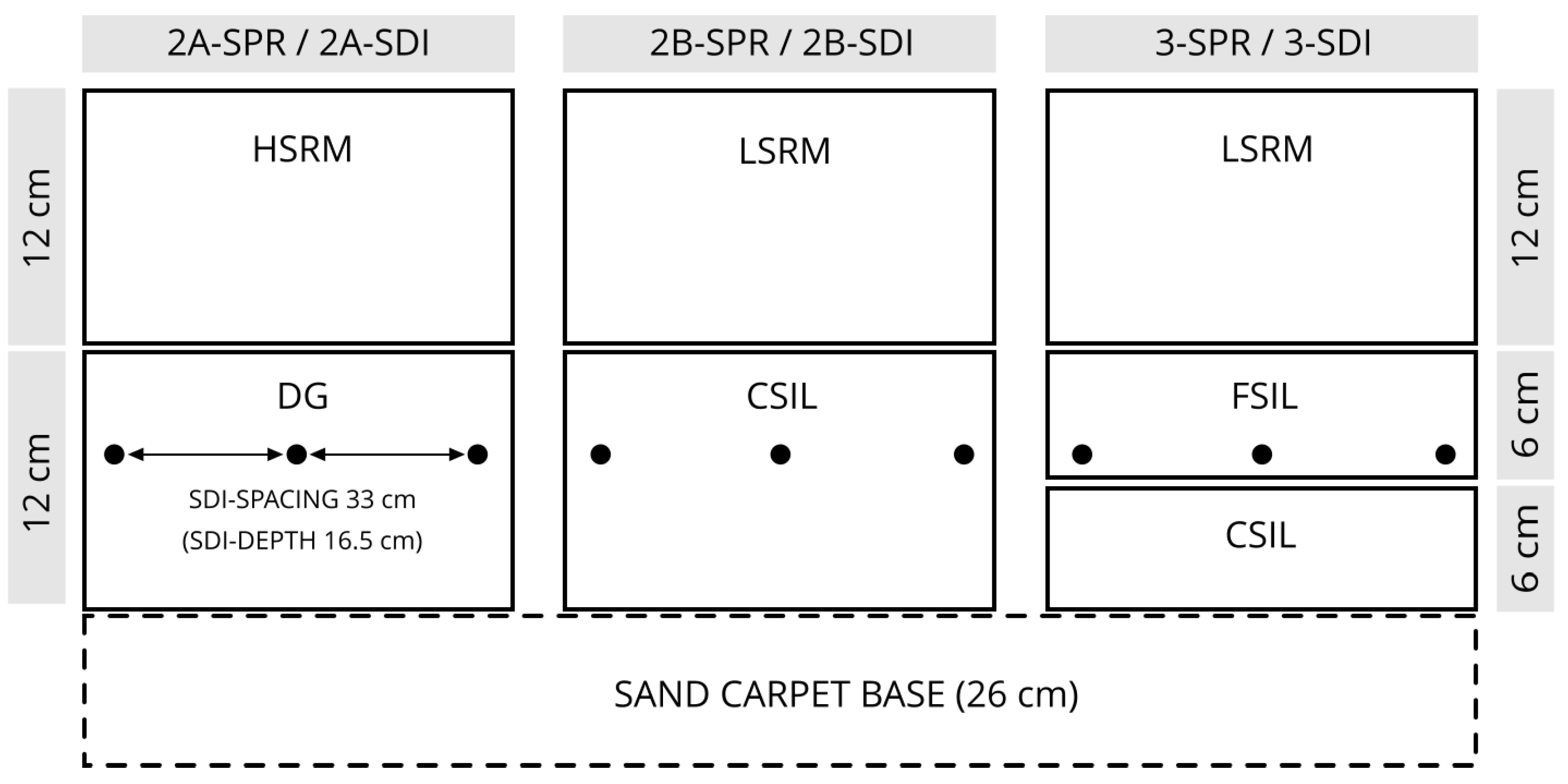
2.1. Materials Used in This Study

This study used three different rootzone construction methods (2A, 2B, and 3) and two different irrigation systems, sprinkler (SPR) and subsurface drip irrigation (SDI), to verify and enhance the model quality and evaluate efficient irrigation management in turfgrass rootzones.

The three 24 cm-deep rootzone construction methods required the use of five materials, and the physical properties of those materials are listed in

Table 1. Overview of the five materials used: HSRM, LSRM FSIL DG, and CSIL, and their associated physical properties.

Material	Physical Properties
	Texture *				Grid (mm)	Bulk Density (g cm−3)	Ks (mm h−1) **	Pore Space (vol.%) ***	Field Capacity (vol.%) ****
	Gravel	Sand	Silt	Clay
	(Mass%)
HSRM	(-)	89.6	10.4	(-)	0–2	1.55	220	41.5	15.9
LSRM	(-)	98.3	1.7	(-)	0–2	1.46	649	44.9	13.6
FSIL	(-)	99.6	0.4	(-)	0.1–0.5	1.41	1465	46.6	6.4
DG	31.5	66.1	2.4	(-)	0–8	1.80	916	32.1	6.5
CSIL	(-)	99.8	0.2	(-)	0.2–2	1.60	6081	39.6	4.6

*: particle size distribution was determined according to [73]. **: hydraulic conductivity K_s was determined in the laboratory according to [74]. ***: pore space was determined from particle density using gas pycnometry [75] and bulk density. ****: field capacity (at pF 1.8) was determined by hanging a water column in a sand bed according to [76].

. The five construction components were: a high silt (≈10%), peat- and topsoil-amended sand-based rootzone mixture (HSRM), a low-silt (≈1%), peat-amended sand-based rootzone mixture (LSRM), a fine-sand intermediate layer (FSIL), a locally sourced drainage gravel (DG), and a coarse-sand intermediate layer (CSIL). A HSRM is generally used for sports turf areas with a common requirement for functionality and sorption capability, as this type of mixture has high functionality at the expense of sorption capability due to having a lower silt content than HSRMs. It also exhibits higher hydraulic conductivity while maintaining a water-holding capacity (field capacity) similar to that of HSRMs. FSILs consist of medium-sized sand (grain size up to 0.5 mm) with very low silt content, and a much higher hydraulic conductivity and lower water-holding capacity (field capacity) than HSRMs and LSRMs. The DG used herein is a drainage gravel with a 0–8 mm particle size distribution, higher hydraulic conductivity, and lower silt content than the rootzone materials (HSRM and LSRM). The CSIL is made of a much finer material, consisting of very coarse sand with a grain size of up to 2 mm, and has a much higher hydraulic conductivity and a lower bulk density than DG.

In accordance with the German Standards for Sports Grounds [71], two of the construction methods had a two-layered design (2A and 2B). Rootzone 2A was 12 cm HSRM over 12 cm DG and rootzone construction method 2B comprised 12 cm LSRM over 12 cm CSIL. Based on the guidelines of the United States Golf Association [77], the third construction method featured a three-layer design consisting of 12 cm of LSRM placed over 6 cm of FSIL which was subtended by 6 cm of CSIL. Each construction method was supported by an underlying 26 cm sand carpet base with a grain size of up to 2 mm for drainage (Figure 1).

In each case, all materials were installed with a bulk density of 95% of the standard Proctor density [71] (HSRM = 1.55, LSRM = 1.46, FSIL = 1.41, DG = 1.80, CSIL = 1.60 g cm⁻³) and two systems for irrigation. Due to the plot size and to maximize the water distribution uniformity, SPR-irrigated plots were hand-watered with a discharge rate of 10 mm h⁻¹. The SDI system used was a line-source drip system consisting of porous pipes (radius r = 0.9 cm) with a discharge rate of 3 L h⁻¹ m⁻¹ (9.09 L h⁻¹ m⁻²) resulting from a line spacing of 33 cm. The SDI installation depth was 16.5 cm, and the operating pressure was 0.2 bar.

2.2. Experimental Setup and Measurements

Experimentally measured data were collected under greenhouse conditions using bare soil profiles (plots with no grass cover). The research area (11.94 m × 4.71 m, including non-considered edge areas of the actual test plots) was designed as a completely randomized two-factorial split plot with three replications for each treatment. The total area comprised six main plots (each 4.11 m × 1.70 m; three for SPR and three for SDI irrigation). Each of the six main plots was divided into three plots (1.70 m × 1.37 m) for the three construction types (two 2-layered and one 3-layered design). Two different irrigation cycles with discharge amounts of cycle 1 = 10 mm (the usual irrigation amount for turfgrass and used for model calibration) and cycle 2 = 20 mm (used for model validation) were applied, both with an intensity of 10 mm h⁻¹. After irrigation cycle 1, all plots underwent a drying phase (approximately four weeks with an average evaporation rate of 3.22 mm day⁻¹) to achieve a uniform initial soil volumetric water content. The initial volumetric water content was between 9 and 10 vol.%, without significant differences between the plots. The collected dataset for each evaluated SPR- or SDI-irrigated variant (2A, 2B, and 3) comprised 30 measurements (n = 30), which were derived from a) three distinct observation depths (3, 6, and 12 cm) and b) ten specific observation times (0.00, 0.17, 0.33, 0.50, 2.00, 4.00, 8.00, 12.00, 24.00, 48.00 h after irrigation initiation). Data were collected in two separate operations during both cycles and, to ensure an identical initial volumetric water content (VWC), irrigation cycle 2 commenced following a drying phase of three weeks. Soil samples were taken with a soil sampler through lateral openings at −3, −6, and −12 cm using a 50 mm-diameter metal tube, which was driven into the soil and withdrawn. The soil gravimetric water content was measured by oven-drying the soil samples at 105 °C, and the VWC was calculated by multiplying it with bulk density. For each replication and observation time, a total of 15 soil samples were collected from five measurement points (center of the plot above the SDI line and at 8.25 and 16.5 cm right and left of the center; at similar positions for the SPR variants) and at depths of 3, 6, and 12 cm. The five water content values for one depth for each sampling were averaged. After sampling, the voids were refilled with the same soil material.

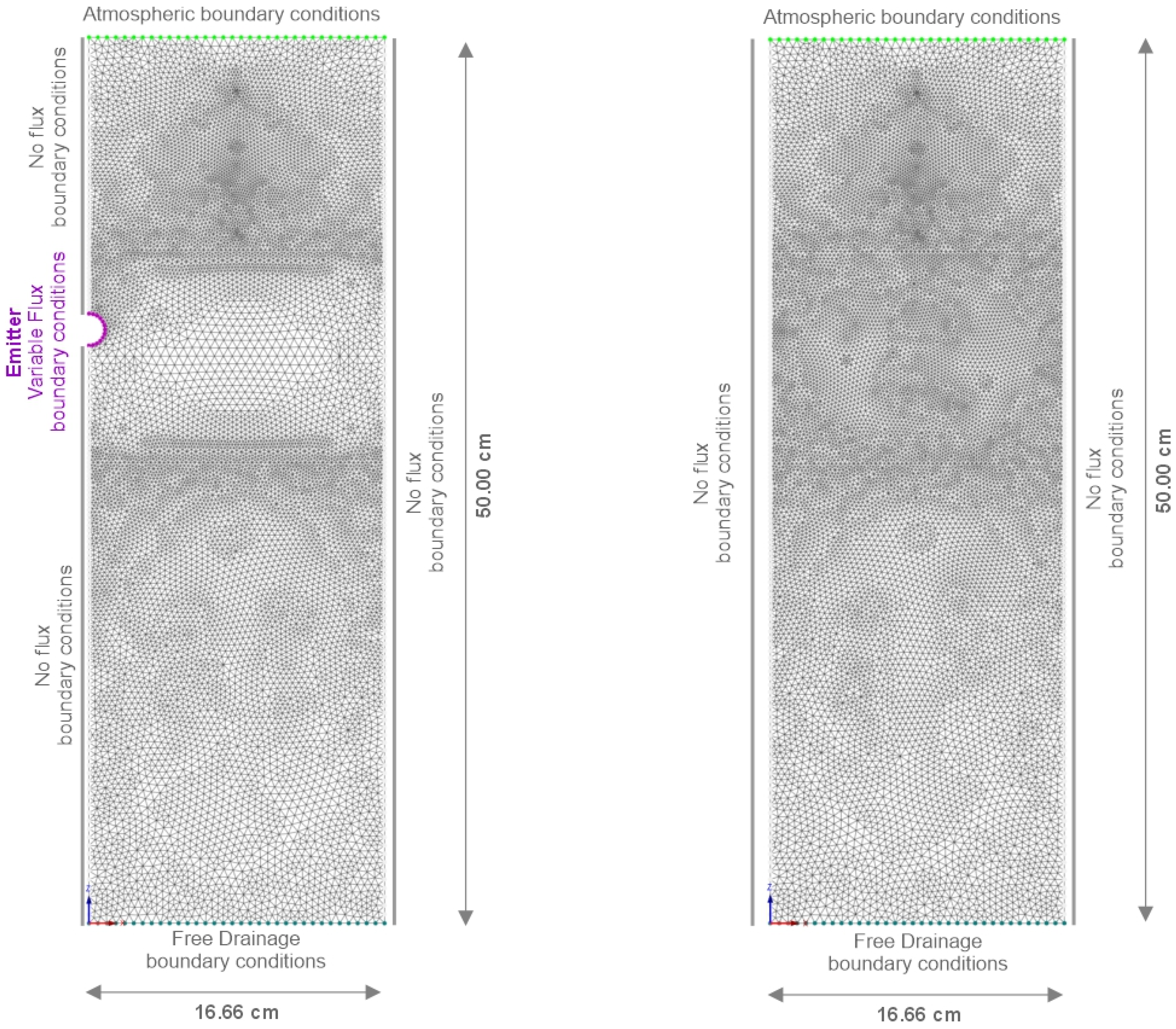
2.3. Simulation Model, Initial and Boundary Conditions

HYDRUS-2D (H2D) finite element model version 5.04 [66], a well-known parametric model that connects volumetric water content to matric potential, as proposed by van Genuchten [46], was employed to simulate the distribution of irrigation water in bare soil profiles. The parametric model incorporates parameters such as ϴ_r, ϴ_s, α, n, and m and is integrated into the HYDRUS-2D model as follows:

$${\mathsf{\theta }}_{\left(\mathsf{\psi }\right)}={\mathrm{ϴ}}_r+{\displaystyle \frac{{\mathsf{\theta }}_{\mathrm{s}}-{\mathsf{\theta }}_{\mathrm{r}}}{{\left(1+{\left|\alpha ·\mathsf{\psi }\right|}^n\right)}^m}}$$

(1)

where ${\mathrm{ϴ}}_{\mathsf{\psi }}$ is the water content at matric potential $\mathsf{\psi }$; ϴ_r is the residual water content (cm³ cm⁻³); ϴ_s is the saturated soil water content (cm³ cm⁻³); α, n, and m describe the shape of the function without physical meaning; and m is usually fixed as 1 − 1/n [54].

The previously discussed formulation can be integrated with Mualem’s equation [49] to elucidate the unsaturated hydraulic conductivity function, and it is also incorporated in the HYDRUS-2D model:

$$K_{\mathsf{\psi }}=K_{\mathrm{s}}·S_e^{ L}·{\left[{1-\left(1-S_e^{ {\displaystyle \frac{1}{m}}}\right)}^m\right]}^2$$

(2)

with

$$Se={\displaystyle \frac{{\mathrm{ϴ}-\mathrm{ϴ}}_r}{{{\mathrm{ϴ}}_s-\mathrm{ϴ}}_r}}$$

(3)

where ${\mathrm{K}}_{\mathsf{\psi }}$ is the hydraulic conductivity at matric potential $\mathsf{\psi }$; K_s is the saturated hydraulic conductivity; S_e is the effective water content; L is a parameter describing the pore structure of the soil, usually set to 0.5; and m is fixed as m = 1 − 1/n [50,51,52].

The simulation was initiated by creating a model setup with the correct material layers, initial conditions, and boundary conditions within H2D that corresponded to the experimental setup. The observed volumetric soil water content in the soil profile was taken as the initial water content for all simulated scenarios. The model’s soil surface was subjected to atmosphere boundary conditions for soil water evaporation (E_V) corresponding to greenhouse conditions with 0.013 cm h⁻¹. A free drainage boundary condition was imposed at the bottom of the soil profile. On the right and left sides of the soil profile, a no-flux boundary was used (Figure 2).

SPR irrigation was scheduled in accordance with the experimental setup with an intensity of 1 cm h⁻¹. For SDI, a variable flux boundary was used around the SDI emitter (Figure 2). During irrigation, the drip pipe boundary had a constant water flux, which was obtained by dividing the emitter discharge flow rate of 3 L (h × m)⁻¹ by the surface of the drip pipe as follows:

$$q={\displaystyle \frac{\mathrm{E}\mathrm{m}\mathrm{i}\mathrm{t}\mathrm{t}\mathrm{e}\mathrm{r} \mathrm{d}\mathrm{i}\mathrm{s}\mathrm{c}\mathrm{h}\mathrm{a}\mathrm{r}\mathrm{g}\mathrm{e} \mathrm{f}\mathrm{l}\mathrm{o}\mathrm{w} \mathrm{r}\mathrm{a}\mathrm{t}\mathrm{e}}{\mathrm{p}\mathrm{i}\mathrm{p}\mathrm{e} \mathrm{s}\mathrm{u}\mathrm{r}\mathrm{f}\mathrm{a}\mathrm{c}\mathrm{e} \mathrm{a}\mathrm{r}\mathrm{e}\mathrm{a}}}=\left({\displaystyle \frac{{{3000 \mathrm{c}\mathrm{m}}^3 \left(\mathrm{h}\right)}^{-1}}{2·0.9 \mathrm{c}\mathrm{m}·\mathsf{\pi }·100 \mathrm{c}\mathrm{m}}}\right)={5.306 \mathrm{c}\mathrm{m}\mathrm{h}}^{-1}$$

(4)

During the no-irrigation period, the flux was kept at zero.

The simulation model domain was 50 cm deep. The high differences between the soil hydraulic parameters of the different materials, as well as the significant temporal-spatial variability under SDI, necessitated a node spacing of 0.50 mm, with progressively closer spacing down to 0.25 mm around the SDI pipe and each layer interface.

2.4. Model Quality Evaluation Criteria

The evaluation of the HYDRUS-2D model encompassed the assessment of model quality, sensitivity analysis, and model calibration based on the predicted and measured volumetric soil water content (VWC) dataset (n = 30) of each variant within the upper 12 cm.

The correlation coefficient (R²), root mean square error (RMSE), mean absolute error (MAE), and Nash–Sutcliffe efficiency (NSE) were calculated using the following equation to assess the model quality parameters:

$${\mathrm{R}}^2={\left({\displaystyle \frac{S_{XY}}{S_X{S}_Y}}\right)}^2$$

(5)

$$RMSE=\sqrt{{\displaystyle \frac{1}{N}}\sum _{i=1}^N{\left(X_i-Y_i\right)}^2}$$

(6)

$$MAE={\displaystyle \frac{1}{N}}\sum _{i=1}^N\left|\left(X_i-Y_i\right)\right|$$

(7)

$$NSE=1-{\displaystyle \frac{{\sum }_{i=1}^N{\left(X_i-Y_i\right)}^2}{{\sum }_{i=1}^N{\left(X_i-X_{av}\right)}^2}}$$

(8)

where S_XY is the covariance between the variables X (measured data) and Y (predicted data). S_X and S_Y are the standard deviations of measured and predicted data, respectively. X_i is the measured data, Y_i = the predicted data, X_av = the average of the measured data, and N = the number of observations.

The correlation coefficient should be close to 1. The root mean square error (RMSE) is a commonly utilized metric for evaluating the agreement between measured and simulated values and should be close to zero. A widely accepted standard that does not consider over- or under-forecasting is the mean absolute error (MAE). In an ideal scenario, the MAE should be nearly zero. Both the root mean square error (RMSE) and mean absolute error (MAE) share the same units as the measured and predicted values [78]. Lastly, the NSE [79] is a normalized statistic commonly used to evaluate hydraulic models which compares residual and measured variance [80]. The parameter equals zero when the square of the differences between the measured and predicted values equals the variability in the measured data. If the NSE value is negative, the measured mean is a more accurate predictor than the model [81]. If the model gives perfect results, the NSE = 1. An acceptable-quality model should have an NSE > 0.5 [54,78].

2.5. Input Parameter, Parameter Sensitivity, Model Calibration and Validation

The water retention drying curves were determined using the Eijkelkamp standard sandbox apparatus [82] to assess the water content at pF 1, 1.8, and 2.5. The water content at pF 4.2 was determined using a pressure plate apparatus, as per the DIN EN ISO 11274 (2019) [76]. The soil water retention curves were then parameterized according to the van Genuchten equation [43] by adjusting the θ_r (residual water content), α, and n (shape factors) values using the EXCEL solver function to match the measured water content and water suction drying curve values. The saturation water content θs was fixed at the total porosity (TP). The material’s hysteretic behavior was evaluated based on the capillary rise of water in the materials employed in this study within experimental containers composed of 10 rigid plastic rings, each measuring 2 cm in height [54]. The rings were filled with the material of interest (95% bulk density of Proctor density D_PR), and a flooding depth of 1 cm was maintained for 48 h before the water content was determined gravimetrically. It was assumed that the water tension in the rings is defined by the distance to the water table, and that the water content at equilibrium is analogous to the water retention curve [50]. The wetting water retention curve was initially parameterized by adjusting the parameter α and defining it as α_w [52]. The analytically determined soil parameters used in HYDRUS-2D are presented in

Table 2. Analytically determined soil parameters used in the HYDRUS-2D program.

Parameters	HSRM	LSRM	FSIL	CSIL	DG
ϴs (cm3 cm−3)	0.415	0.430	0.466	0.394	0.321
ϴr (cm3 cm−3)	0.060	0.076	0.011	0.014	0.014
Ks (cm h−1)	22.019	64.854	146.474	608.12	91.612
α	0.089	0.061	0.055	0.228	0.085
αw	0.118	0.119	0.077	0.300	0.156
n	1.728	2.090	2.719	1.929	2.063
l	0.5	0.5	0.5	0.5	0.5

.

Sensitivity analyses and model calibration focused on the materials used in the top two layers, including HSRM, LSRM (rootzone layers), FSIL (intermediate layer), and DG (drainage gravel layer) within each construction method (2A, 2B, and 3) and irrigation system (SDI and SPR). The HYDRUS-2D model was used to analyze the sensitivity of the soil hydraulic parameters θ_r, α, and n (representing the soil water retention drying curve parameterization) while excluding the exact analytically determinable parameter θ_s (fixed at total porosity), as well as the parameters α_w and θ_s^w (representing the opportunities in the HYDRUS code for describing a material’s hysteresis behavior). This study evaluated the impact of a 20% incremental increase in these parameters on the simulation output (VWC) after 10 mm irrigation (cycle 1), regarding the deviation in model efficiency (NSE).

For model calibration, the Levenberg–Marquardt optimization algorithm [83], in conjunction with the HYDRUS-2D code [41], was employed to inversely estimate the desired soil hydraulic parameters. These parameters were determined through the systematic minimization of differences between observed and simulated state variables (i.e., VWC). The total differences are expressed by an objective function, $\varphi$, which may be defined as [84]:

$$\varphi \left(\beta , \gamma \right)=\sum _{j=1}^{j=m_y}{v}_j \sum _{i=1}^{i=n_j}{w}_{i,j}\left[y_i^{*}\left({z,t}_i\right)-y_i\left({z,t}_i,\beta \right)\right]2$$

(9)

where the right side represents the residuals between the measured ${(y}_i^{*})$ and corresponding model-predicted ${(y}_i)$ space-time variables using the soil hydraulic parameters of the optimized parameter vector, $\beta$. The initial summation aggregates the residuals for all measurement types ${(m}_y)$ (i.e., VWC), whereas the variable $n_j$ in the subsequent summation denotes the number of measurements for a specific measurement type, $j$. Assuming that measurement errors within a given measurement type are independent and uncorrelated, the weighting factor values for $v_j$ can be chosen to ensure either equal weighting of data types through a normalization procedure or weighting proportional to the reciprocal of the measurement variance for type $j$ [85].

The model calibration process involved (i) separately calibrating the four soil hydraulic parameters identified as most sensitive through sensitivity analysis (scenarios F1–F4) and (ii) simultaneously calibrating, based on previous research [48,52,64,65], the shape parameters α_w and n (scenario F5) as well as α_w and ϴ_s^w (scenario F6). In total, six distinct and independent scenarios (F1–F6) were utilized for the calibration procedures, each without internal weighting of inversion data.

Following calibration, the most suitable model for simulation was identified and subsequently validated using an independent dataset (irrigation cycle 2). This validation step was conducted to evaluate the model’s reliability.

2.6. Irrigation Management Principles

The HYDRUS-2D code was also used in hypothetical instances to examine the effects of irrigation treatments, which are given in

Table 3. Irrigation management parameters within the four irrigation approaches (1–4) under SPR, SDI, and HYBRID (SPR + SDI) irrigation across construction method 3.

Irrigation Approach	Irr. Events Within 12 h	Water Applied per Charge (mm)					Proportion
		0	3	6	9	12	SPR	SDI
(-)	(-)	Hours					(%)	(%)
SPR-1	1	10.00	0	0	0	0	100	0
SPR-2	2	7.50	0	2.50	0	0	100	0
SPR-3	3	5.00	0	2.50	0	2.50	100	0
SPR-4	4	5.00	1.25	1.25	1.25	1.25	100	0
SDI-1	1	10.00	0	0	0	0	0	100
SDI-2	2	7.50	0	2.50	0	0	0	100
SDI-3	3	5.00		2.50		2.50	0	100
SDI-4	4	5.00	1.25	1.25	1.25	1.25	0	100
HYBRID-1	1	5.00 (SPR), 5.00 (SDI)	0	0	0	0	50	50
HYBRID-2	2	7.50 (SPR)	0	2.50 (SDI)	0	0	75	25
HYBRID-3	3	5.00 (SPR)	0	2.50 (SDI)	0	2.50 (SDI)	50	50
HYBRID-4	4	5.00 (SPR)	1.25 (SDI)	1.25 (SDI)	1.25 (SDI)	1.25 (SDI)	50	50

. The parameters for the boundary and flow domain remained unchanged from previous descriptions. Based on previous research [86,87] that demonstrated the favorable water retention characteristics of the three-layered construction method 3, this methodology was employed to evaluate the efficacy of various irrigation approaches regarding water usage.

The analysis focused on two key factors that influence irrigation efficiency, i.e., drainage flux and soil water storage within the simulation domain (upper 50 cm). Four different irrigation approaches were assessed. Each approach involved applying a total irrigation amount of 10 mm through either SPR (SPR 1–4), SDI (SDI 1–4), or HYBRID (HYBRID 1–4) over up to five irrigation events within a 12 h period.

3. Results

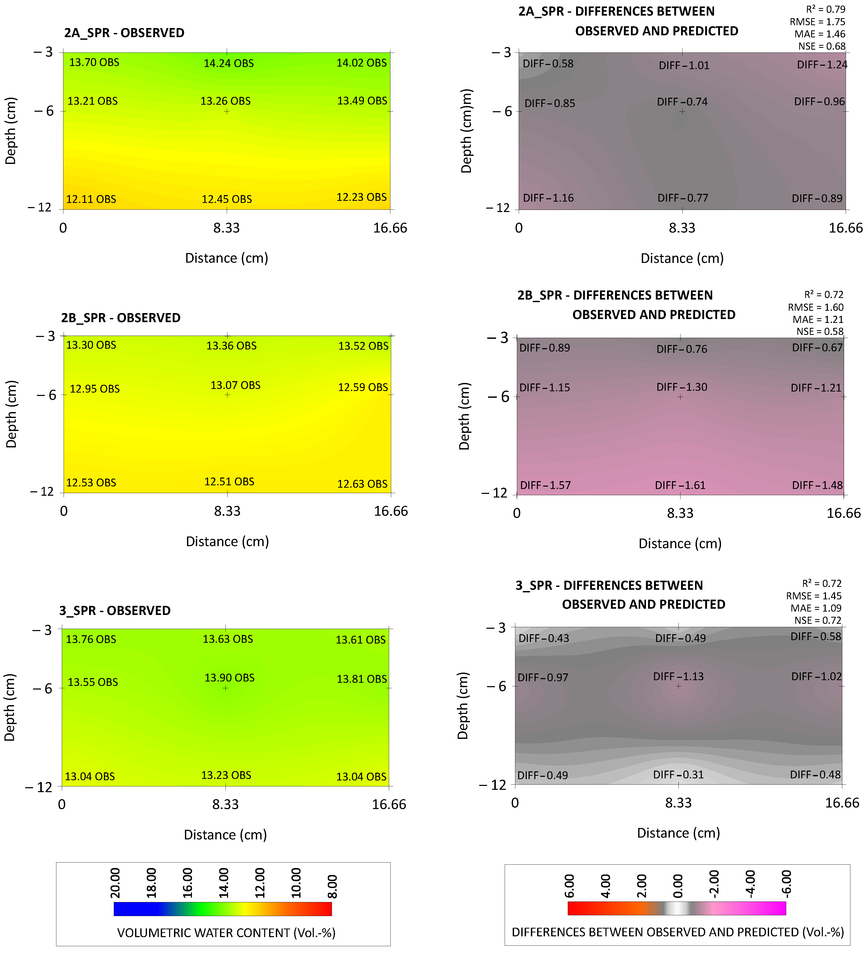
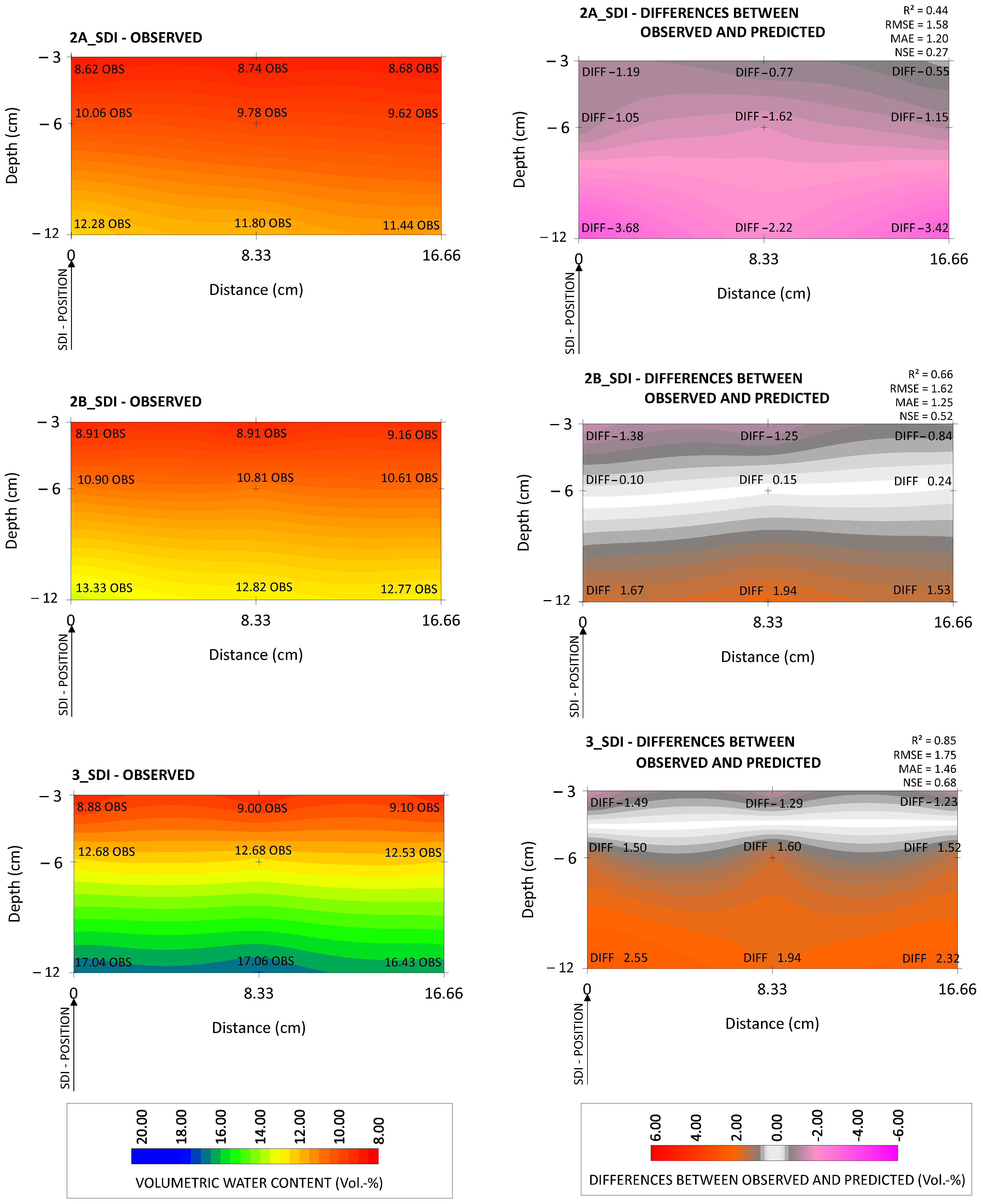
3.1. Model Quality Evaluation

The uncalibrated model’s performance was evaluated using the model efficiency parameter (NSE). Further, the results were graphically visualized by comparing the observed values against the simulation output differences and are presented through spatial maps (ordinary Kriging method).

Figure 3 compares the observed values (left) and the difference values (right) of construction methods 2A, 2B, and 3 under SPR irrigation, each averaged across the entire observation time of 0–48 h following 10 mm irrigation. Figure 4 is analogous to Figure 3, but shows each case under SDI. The NSEs of the uncalibrated models ranged from 0.27 (2A_SDI) to 0.72 (3_SPR), with the SPR variants generally achieving NSEs above 0.5.

Graphical analysis showed that, for the SPR variants 2A and 2B, the model tended to calculate predicted values that were higher than the observed values. At an observation depth of 6 cm, the average overestimation was 0.85 vol.% for 2A and 1.22 vol.% for 2B. At a depth of 12 cm, the average overestimation was 0.94 vol.% for 2A and 1.55 vol.% for 2B. In the case of the SDI system, average overestimations within variant 2A of 1.27 vol.% (6 cm depth) and 3.11 vol.% (12 cm depth) were observed. In contrast, variant 3_SDI exhibited a different pattern, with the model generating predicted values that were lower than the observed ones. The average underestimation was 1.54 vol.% at a depth of 6 cm and 2.27 vol.% at a depth of 12 cm. Similar to the model’s performance, variant 3 showed the most minor differences among the SPR variants, while 2B displayed the least variation among the SDI variants.

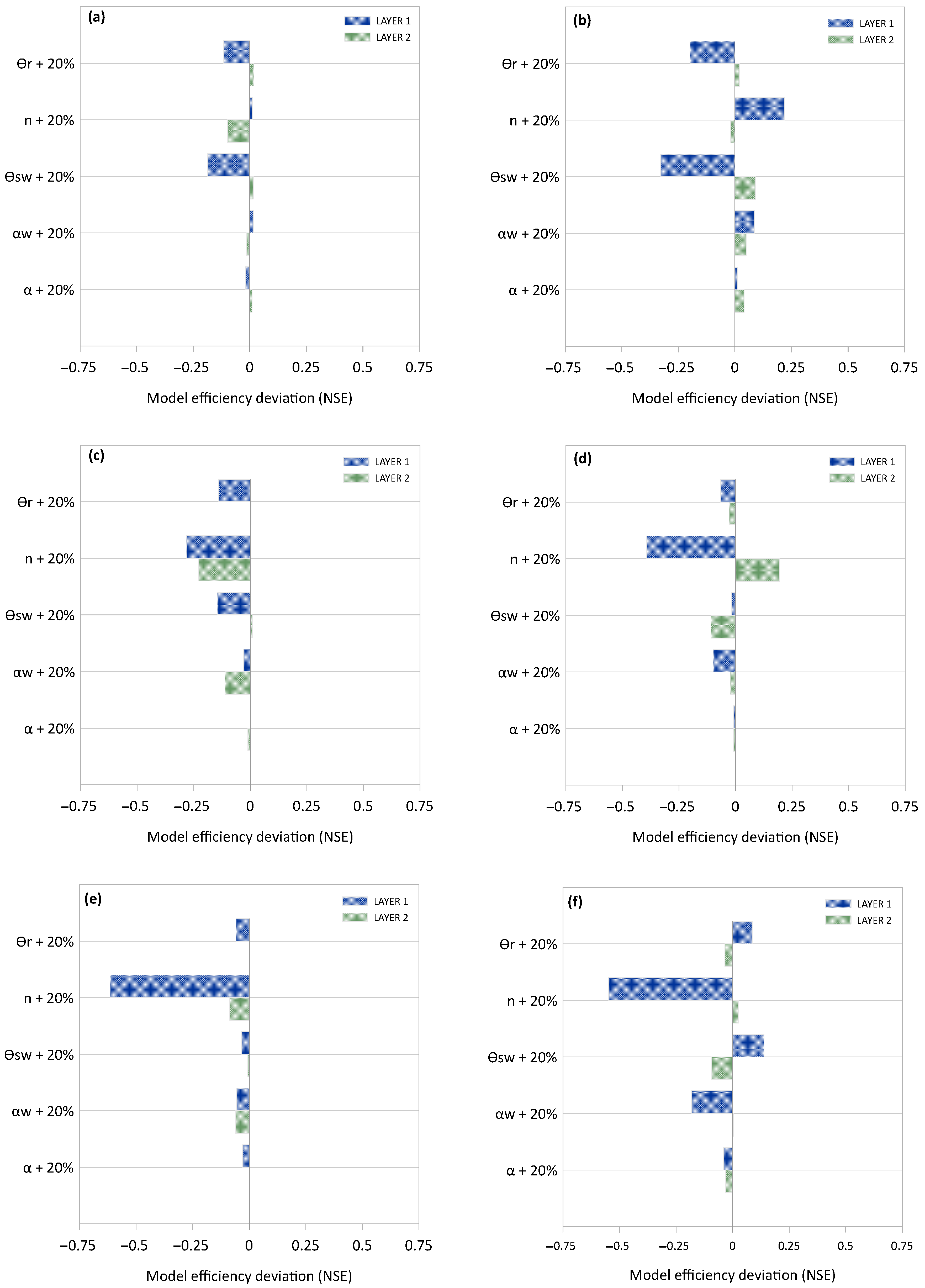
3.2. Sensitivity Analysis

The sensitivity analyses of the five parameters, ϴ_r, α, n (normal drying WRC), ϴ_s^w, and α_w (wetting WRC), presented in Figure 5 illustrate the respective deviations in model efficiency (NSE) under a soil hydraulic parameter perturbation of +20% within each variant’s upper two layers (Layer 1 and Layer 2).

The results demonstrated that the parameter perturbation elicited contrasting sensitivity responses across the evaluated variants. Generally, it could be observed that the materials within Layer 1 reacted more sensitively under a soil hydraulic parameter alteration compared to Layer 2, with an average NSE increase (absolute value across all parameters and variants) of 0.14 compared to 0.05, respectively (Table S1 in the Supplementary Materials). Further, among the five parameters that were examined, α consistently exhibited the least sensitivity with maximum NSE deviations of −0.04 (3_SDI, Layer 1) and 0.04 (2A_SDI, Layer 2), while parameter n demonstrated the highest sensitivity with a maximum NSE deviation of −0.62 (3_SPR, Layer 1). An analysis of the variations in parameter n revealed that four out of the six variants in both layers showed negative NSE deviations. The exceptions were variants 2A_SPR and 2A_SDI in Layer 1 and 2B_SDI and 3_SDI in Layer 2. Parameter ϴ_s^w had the second highest sensitivity, and its NSE deviation ranged from 0.14 (3_SDI) to −0.33 (2A_SDI) in Layer 1 and from 0.09 (2A_SDI) to −0.11 (2B_SDI) in Layer 2. In summary, based on the absolute averaged NSE deviation (across all parameters and variants), the four most sensitive parameters are as follows (Table S1 in the Supplementary Materials):

n (0.35) > ϴ_s^w (0.14) > ϴ_r (0.11) > α_w (0.04) within Layer 1;

n (0.11) > ϴ_s^w (0.05) > α_w (0.04) > ϴ_r (0.02) within Layer 2.

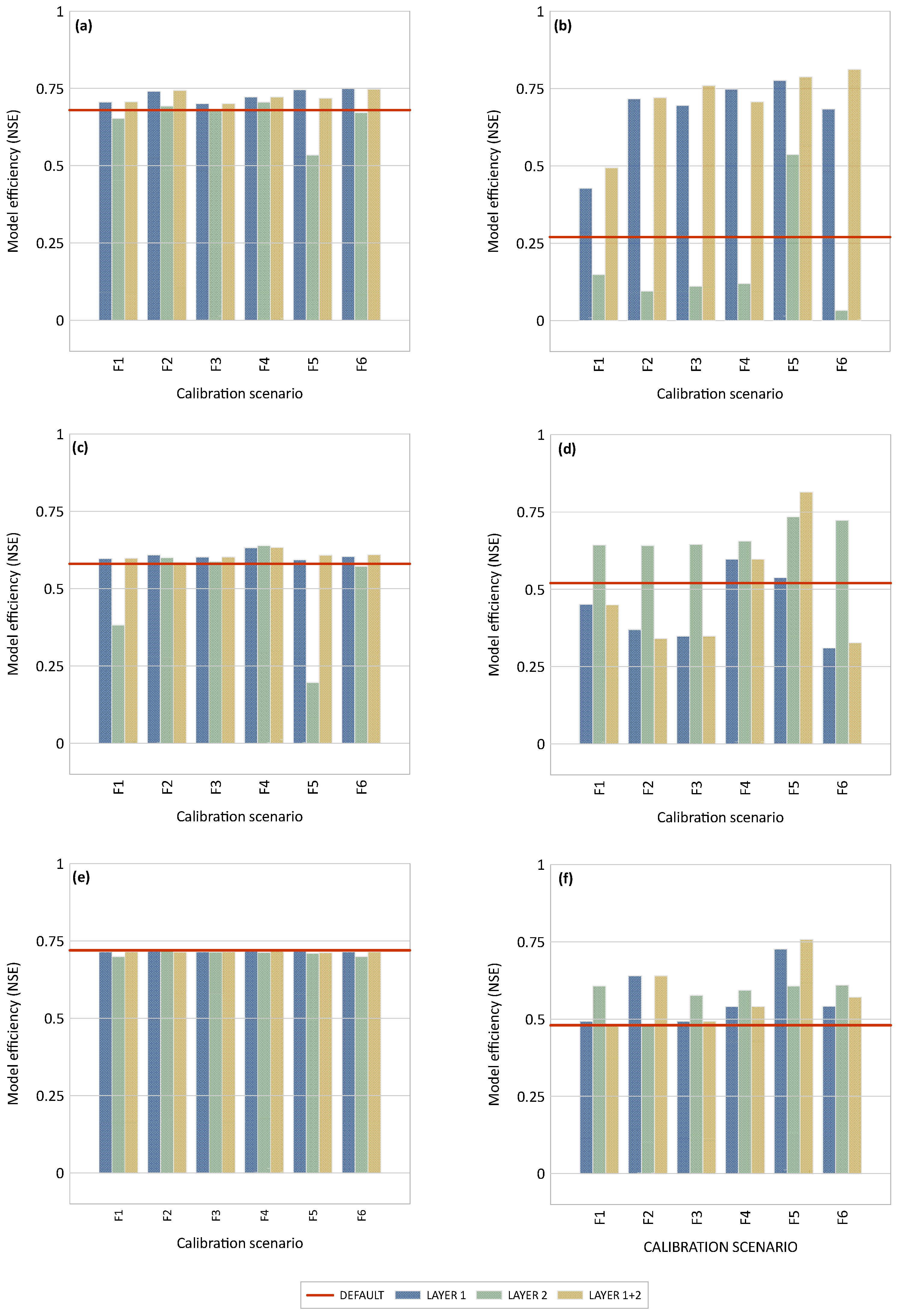
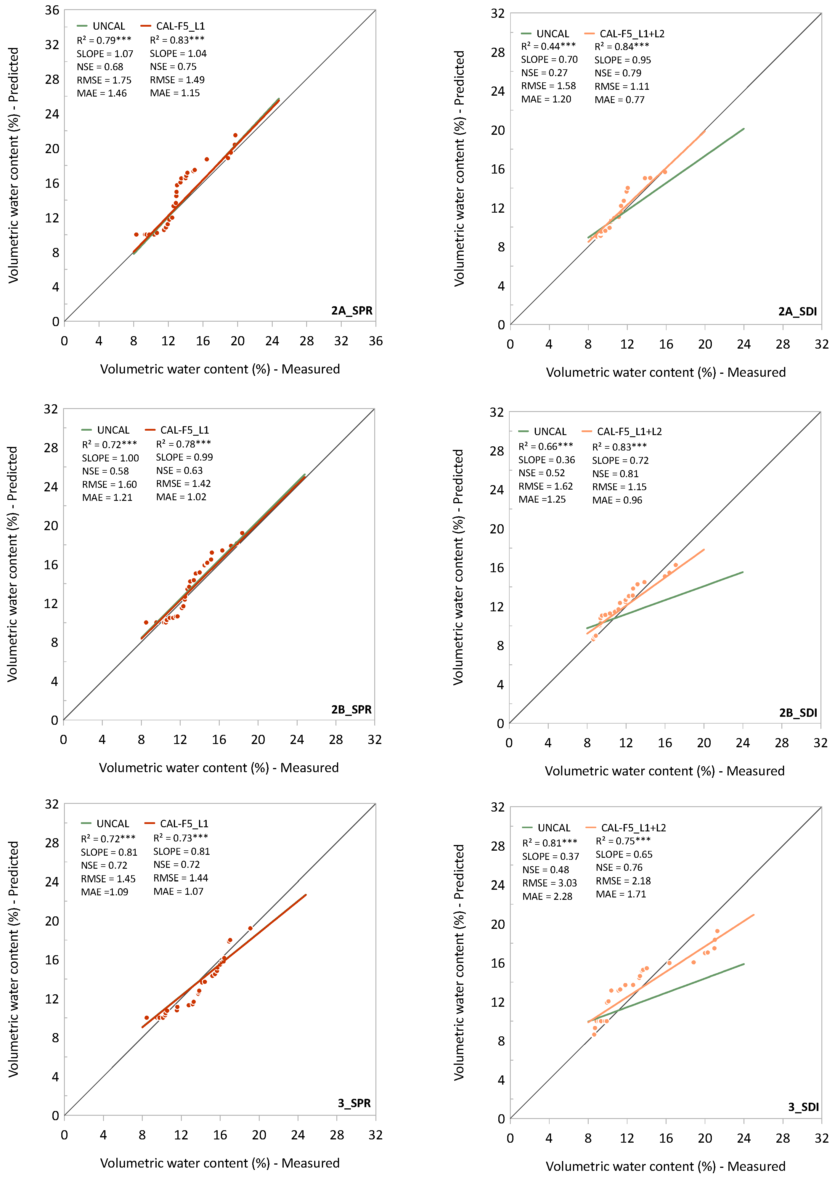
3.3. Model Calibration

The results of the model calibration, calculated using the HYDRUS-2D inverse solution, are presented for each material (HSRM, LSRM, DG, and FSIL) and scenario (F1–F6) in

Table 4. Results of the HYDRUS inverse solution of the van Genuchten parameters within the six model calibration scenarios (F1–F6) for Layer 1 (rootzone HSRM and LSRM) and Layer 2 (drainage gravel layer DG and intermediate layer FSIL) across construction methods 2A, 2B, and 3 employing SPR or SDI systems.

Layer	Material	* CM	** IS	F1	F2	F3	F4	F5		F6
				αw	n	ϴsw	ϴr	αw	n	αw	ϴsw
				(-)		(cm3 cm−3)		(-)		(-)	(cm3 cm−3)
1	HSRM	2A	SPR	0.147	1.842	0.402	0.056	0.144	1.833	0.164	0.382
			SDI	0.152	2.076	0.306	0.035	0.109	2.095	0.145	0.311
	LSRM	2B	SPR	0.127	2.153	0.420	0.073	0.131	2.052	0.131	0.430
			SDI	0.136	2.306	0.322	0.058	0.117	2.110	0.128	0.329
		3	SPR	0.119	2.080	0.430	0.076	0.119	2.084	0.119	0.430
			SDI	0.119	1.905	0.430	0.074	0.121	1.826	0.103	0.430
2	DG	2A	SPR	0.152	1.983	0.321	0.013	0.203	1.764	0.166	0.321
			SDI	0.388	2.076	0.240	0.011	0.207	3.005	0.207	0.241
		2B	SPR	0.129	1.881	0.321	0.022	0.116	2.199	0.097	0.121
			SDI	0.155	2.042	0.321	0.014	0.202	2.332	0.154	0.321
	FSIL	3	SPR	0.076	2.662	0.466	0.023	0.077	2.671	0.077	0.466
			SDI	0.083	2.719	0.466	0.011	0.079	2.720	0.087	0.466

NOTE. * construction method; ** irrigation system.

. The influence of model calibration scenarios F1–F6 on the model efficiency (NSE) is illustrated in Figure 6.

Notably, substantial variations are observed depending on whether the calibration is incorporated into Layer 1 (L1) or Layer 2 (L2) or if it is implemented across both upper layers, Layer 1 and 2 (L1 + L2). In general, the SPR variants, which already exhibited NSEs exceeding 0.50 under the laboratory-measured default settings, demonstrated only a minor improvement across all model calibration scenarios (up to +0.07). Nevertheless, analyses across the SPR variants indicated that calibration scenario F5_L1 exhibited the highest improvement, with an average NSE value of 0.70 (Table S2 in the Supplementary Materials). Within the SDI variants, generally, model calibration scenario F5 pushed the NSE values to a range of > 0.50, whereby the greatest improvement could be achieved with the combined implementation of both layers (L1 + L2), and the values increased in 2A_SDI from 0.27 to 0.79, in 2B_SDI from 0.52 to 0.81, and in 3_SDI from 0.48 to 0.76. The impacts of the model calibration scenarios on the average NSE values across the SDI variants were ranked in descending order as follows (details in Table S2 in the Supplementary Materials): F5_L1 + L2 (0.79) > F5_L1 (0.68) > F5_L2 = F4_L1 (0.63).

To sum up, scenario F5 (i.e., calibration α_w and n) involving Layer 1 for the SP system R and both upper layers for the SDI system resulted in the highest gain in model efficiency in this study. Subsequently, we assessed the model validation with data from irrigation cycle 2 (20 mm of irrigation in a period of 2 h followed by redistribution period of 46 h), which revealed the reliability of the calibrated parameters, indicated by NSE values of 0.71 (2A_SPR), 0.69 (2B_SPR), 0.73 (3_SPR), 0.70 (2A_SDI), 0.83 (2B_SDI), and 0.71 (3_SDI).

Figure 7 presents model quality parameters and a regression analysis of the measured values (n = 30) in comparison with the simulated VWC across the uncalibrated (UNCAL) and calibrated (CAL) models, incorporating scenario F5_L1 for the SPR variants and scenario F5_L1 + L2 for the SDI variants. The correlation coefficient (R²), RMSE, and MAE values across the SPR variants were between 0.72 and 0.79, 1.45 and 1.75 vol.%, and 1.09 and 1.46 vol.%, respectively, under the default settings and developed to 0.73–0.83, 1.42–1.49 vol.%, and 1.02–1.15 vol.%, respectively, under model calibration scenario F5_L1. Within the SDI variants, the values were between 0.44 and 0.81, 1.58 and 3.03 vol.%, and 1.20 and 2.28 vol.%, respectively, under the default settings and developed to 0.75–0.84, 1.11–2.18 vol.%, and 0.77–1.71 vol.%, respectively, under model calibration scenario F5_L1 + L2.

Generally, the correlation coefficients (R²) were greater across the calibrated SDI variants (0.75–0.84) than across the calibrated SPR variants (0.73–0.83). Nevertheless, the slopes of the regression lines were closer to 1 within the SPR variants compared to the SDI variants and ranged from 0.81 (3_SPR) to 1.04 (2B_SPR) and from 0.65 (3_SDI) to 0.95 (2A_SDI), respectively.

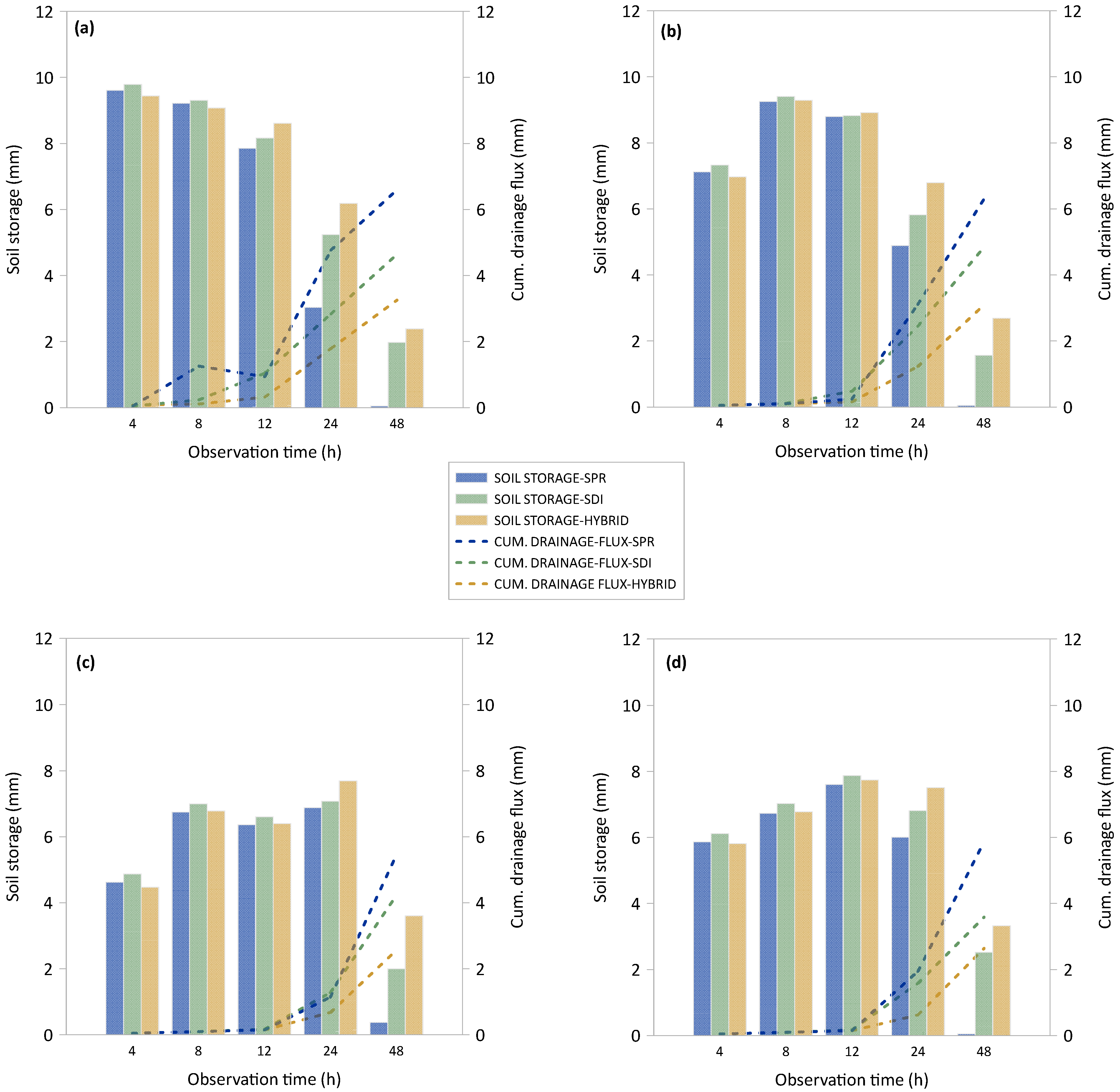
3.4. Irrigation Management Evaluation

The results of the HYDRUS-2D code of the three-layered construction method 3, which were utilized in hypothetical instances to examine four different irrigation approaches (IA1: 10 mm irrigation at time zero; IA2: 75% at time 0 and 25% after 6 h; IA3: 50% at time 0 and 25% each after 6 and 12 h; IA4: 50% at time 0 and 12.5% after 3, 6, 12, and 18 h; see Table 4). The results are shown in Figure 8 (and Table S3 in the Supplementary Materials).

These observations were made at various times (4–48 h) after 10 mm irrigation (SPR, SDI, or hybrid). Different behavior concerning the soil storage of irrigation water and drainage flux was observed across the irrigation approaches.

Up to 12 h (8 h for IA1), the water storage (topmost 50 cm of soil) was very similar within the irrigation approaches, with a tendency of generally minimal higher water storage in the SDI variants. Generally, the water storage was higher in IA1 and IA2 compared to IA3 and IA4. Strong differences could be identified between the water storage in the different irrigation systems after 24 h: the SPR variant always showed the lowest water storage followed by the SDI irrigation. The hybrid irrigation system always had the highest water storage. The hybrid-approach results at 48 h were 3.33 mm (IA4), 3.61 mm (IA3), 2.69 mm (IA2), and 2.39 mm (IA1) (Figure 4). Since the cumulative drainage is naturally determined by the water storage, these values were always inversely related to the storage (Figure 4).

In summary, focusing on the maximum residual soil water storage and minimum drainage flux of each irrigation technique (SPR, SDI, HYBRID) and approach (IA1–IA4) at an observation time of 48 h, the following order was observed for soil water storage:

HYBRID-IA3 (3.61 mm) > SDI-IA4 (2.53 mm) > SPR-IA3 (0.38 mm).

Foror drainage flux:

HYBRID-IA3 (2.57 mm) < SDI-IA4 (3.59 mm) < SPR-IA3 (5.46 mm).

The difference in water storage plus drainage flux of the 10 mm irrigation is due to the actual evaporation during the 24 h experiment.

4. Discussion

Turfgrass areas, including golf courses and sports fields, provide essential ecosystem services such as carbon sequestration, oxygen production, water purification, and heat dissipation, contributing to climate change mitigation and urban environmental quality [1,2,88]. Irrigation management must support efficient irrigation water usage, uniform soil moisture distribution, and adequate soil moisture retention to maintain acceptable turfgrass quality. This study evaluated the effectiveness of the HYDRUS-2D model in simulating irrigation water distribution, demonstrating its effectiveness while highlighting the need for calibration in multilayered rootzone construction methods, particularly under SDI irrigation.

4.1. Theoretical Aspects

The model performance varied depending on the construction method and the irrigation system used. The initially uncalibrated model utilizing analytical determined soil hydraulic parameters already demonstrated an acceptable performance for the SPR variants (NSE 0.58–0.72) but a suboptimal performance for the SDI variants (NSE 0.27–0.52). The model tended to overestimate the two-layered SPR and SDI variants, consistent with Ghazouani et al. [89], who reported the overestimation of modeled water content values compared to measured values, with 2A_SDI displaying the lowest model accuracy. In contrast, the three-layered SDI variant notably underestimated the soil water content, particularly in the lower parts of the rootzone (observation depths of 6 and 12 cm).

Sensitivity analysis of the parameters indicated that the shape factor n exhibited the highest sensitivity within both layers and across all variants, whereas shape factor α (drying WC) demonstrated the lowest sensitivity, which is consistent with the results of Inoue et al. [68]. The soil hydraulic parameter ϴ_s^w showed the second highest sensitivity, aligning with the findings of Abbasi et al. [69]. The sensitivity analysis further demonstrated the need for the precise parameterization of soil hydraulic parameters, as construction method 2B/Layer 2 exhibited a decrease in its NSE value of −0.23 when the shape factor n was increased by 20% under SPR irrigation. In contrast, this modification increased the NSE value to +0.19 under SDI irrigation (Figure 5).

The soil hydraulic parameters for each material were independently calibrated using the HYDRUS inverse solution method across the calibration scenarios F1–F6. However, the results demonstrated that the model structure significantly influenced the calibrated materials’ soil hydraulic properties.

Generally, the calibrated α_w (wetting WRC) values resulted in α_w/α ratios averaging 1.90 across all variants (calibration scenario F1), indicating substantially greater α_w values than the corresponding drying curve values. This finding aligns with the study of McCoy and McCoy [48] and approximates the value of 2 (α_w/α ratio) suggested by Kool and Parker [64] for estimating the wetting curve parameter α_w. This supports using this approximation when measured wetting curve data are unavailable.

Nevertheless, the observations indicated that, particularly under a two-parameter simultaneous calibration (scenario F5 and F6), the model’s estimated inverse solution parameters exhibited high variability, notably in Layer 2 and material DG. The values of the factor ϴ_s^w were 0.121 and 0.321 cm³ cm⁻³ within scenario F6 and material DG. Shape factor n showed changeable behavior with a partially low or strongly pronounced increase or decrease depending on the construction method and associated irrigation system, with values ranging between 1.764 and 3.005 (scenario F5, material DG); these findings do not agree with the results of McCoy and McCoy [48], which showed generally lower n values when considering the typical characteristics of the hysteresis wetting curve response. Even under single-parameter calibration (scenario F2, material DG), the values for parameter α_w ranged from 0.152 to 0.388 (Table 4).

These adjustments likely represent the model’s attempt to compensate for errors (differences between observed and predicted VWC) in Layer 1. Given this perspective, prior to utilizing calibrated values that yield the highest improvement in model efficiency, it is imperative to ascertain whether these calibrated parameters fall within a physically plausible range, especially in the context of directly measurable parameters (i.e., ϴ_r and ϴ_s). Furthermore, our findings suggest that, specifically under SDI conditions, the shape parameter n_w (wetting curve) should be additionally considered within the HYDRUS code to more accurately characterize the hysteresis behavior of the material and facilitate a shape factor-based model calibration approach.

Furthermore, the models revealed pronounced gradients at the interface between neighboring layers (Layers 1 and 2) due to the markedly different physical soil properties of the materials employed. For instance, in construction method 3, Layer 1 (HSRM) demonstrated a saturated hydraulic conductivity (K_s) of 649 mm h⁻¹, while Layer 2 (FSIL) showed a value of 1465 mm h⁻¹. Similarly, substantial water content and water suction gradients were observed at the interface of Layers 1 and 2 in construction method 2A, where Layer 1 exhibited a K_s of 220 mm h⁻¹ and Layer 2 had a K_s of 916 mm h⁻¹. These findings indicate that complex model structures involving multilayered rootzone construction methods comprising adjacent layers with significantly different physical soil properties necessitate model calibration, particularly under SDI conditions.

Notwithstanding the observed local variations, the NSE values consistently remained positive, indicating substantial agreement between the measured soil water content and the model’s simulated values [79] despite the complexity of the conditions to which the model was subjected, that is, multi-layered rootzone construction methods and irrigation systems with high spatial variability.

Following calibration, the model strongly agreed with the measured data, achieving NSEs up to 0.81 for the SDI and 0.75 for the SPR variants. The calibration demonstrated that the SPR variants exhibited NSE values > 0.5 even under uncalibrated conditions. Nevertheless, if calibration for further improvement is to be conducted, the results indicated that the consideration of Layer 1 across SPR variants is sufficient (Figure 6). In contrast, under SDI irrigation, a significant improvement in model quality could be observed by considering both layers (Layers 1 and 2). A plausible explanation is that, during SDI irrigation, the model primarily utilized the wetting retention curve in Layer 2. However, during drainage and redistribution, both layers, their corresponding wetting and drying curves, and the connections between them necessitated consideration within the model calibration procedure.

4.2. Practical Significance

Despite discrepancies between the calculated and measured values of the soil water content, these variations typically remained below 4 vol.% and are consistent with standard field measurement uncertainties. These uncertainties are significantly influenced by the specific measurement technology employed (e.g., measurement with a frequency domain reflectometry (FDR) sensor), the measurement point’s location, and the measurement’s timing. Regarding practical significance, it is essential to note that the model demonstrates efficacy in multilayer construction methods with highly complex soil–physical relationships and under irrigation systems with considerable spatial variability (i.e., SDI) that significantly influences irrigation water dynamics [90]. Consequently, this tool facilitates the adaptation of irrigation management to the specific onsite structural conditions of sports turf areas and enables the implementation of efficient irrigation practices.

In the context of irrigation management evaluation, the model data of the three-layered variant (construction method 3) indicated that, under SPR irrigation, dividing the total irrigation water quantity into multiple smaller applications (approaches 3 and 4) generally resulted in higher soil water storage and lower drainage flux compared to single large applications. Furthermore, the model data under the hybrid irrigation approach indicated the most efficient use of resource water, characterized by the highest soil water storage and lowest drainage flux compared to the other irrigation approaches (Figure 8). The practical applicability or the requirement profile of an irrigation technique should also be emphasized, as the maintenance practices typically conducted on turfgrass areas necessitate surface irrigation (i.e., SPR) for establishing seeding or flushing in granulated fertilizers. In the context of turfgrass irrigation, the primary focus remains on the targeted application of irrigation water into the root zone, which should ideally be applied with minimized evaporation loss, surface runoff, and moisture penetration of the turf to reduce disease pressure. The results indicate that, under a hybrid irrigation approach, these requirements are attainable, further demonstrating the potential of HYDRUS-2D as a cost-effective and valuable tool for evaluating and optimizing turfgrass irrigation management.

4.3. Limitations of the Study and Further Research

While the calibrated models exhibited strong overall performance, some discrepancies between the measured and predicted values remained, particularly for the three-layered construction under SDI irrigation. This suggests that further refinement of the HYDRUS code, such as implementing n_w as an additional shape factor, may be necessary to more precisely account for the material’s hysteresis behavior. Moreover, to evaluate the fundamental model performance across various rootzone construction methods and irrigation systems, this study also evaluated bare soil profiles, and found that the incorporation of turfgrass and its associated root water uptake patterns would undoubtedly influence water distribution and irrigation efficiency.

Future research should incorporate root water uptake models to provide a more comprehensive understanding of soil–plant–water dynamics and relationships in using multi-layered construction methods for turfgrass areas, wherein an increasing complexity for model calibration could be anticipated.

5. Conclusions

This study demonstrated the efficacy of the HYDRUS-2D model in simulating irrigation water distribution across various turfgrass rootzone construction methods. The key findings include the following: (i) The initial model performance varied depending on the construction method and irrigation system, with an acceptable to high performance for the SPR variants (NSE 0.58–0.72) but a suboptimal performance for the SDI variants (NSE 0.27–0.52). (ii) Sensitivity analysis revealed that the shape factor n exhibited the highest sensitivity, whereas the shape factor α showed the lowest sensitivity across all variants. Model calibration significantly improved the performance of the model, achieving NSEs up to 0.81 for the SDI and 0.75 for the SPR variants, respectively. This calibration appears necessary, particularly under SDI irrigation, to enhance the model quality in evaluating multilayered rootzone construction methods. The calibrated α_w/α ratios averaged 1.90 across all variants, aligning with previous research and supporting the use of this approximation when the measured wetting curve data are unavailable. (iii) The evaluation of irrigation management revealed that dividing the total irrigation water quantity into multiple smaller applications generally resulted in higher soil water storage and lower drainage flux than single large applications. (iv) A hybrid irrigation approach combining SPR and SDI systems exhibited the most efficient use of water resources.

While the calibrated models demonstrated good overall performance, some discrepancies between the measured and predicted values persisted, particularly for the three-layered construction under the SDI system. This finding suggests that further refinement of the model is necessary. These findings indicate that HYDRUS-2D has the potential to be an efficient tool for evaluating irrigation strategies in turfgrass areas. However, future research should incorporate root water uptake models to provide a more comprehensive understanding of soil–plant–water dynamics in using multilayered construction methods for turfgrass areas.

Overall, this modeling approach has the potential to optimize irrigation management in turfgrass rootzones, thereby enhancing water-use efficiency and minimizing resource wastage. Consequently, this optimization improves the sustainability, capacity for carbon sequestration, and provision of ecosystem services of turfgrass, which are particularly crucial in urban settings.

References

1. Beard, J. Turfgrass: Science and Culture; Prentice-Hall Inc.: Englewood Cliffs, NJ, USA, 1973. [Google Scholar]
2. Beard, J.B.; Green, R.L. The role of turfgrasses in environmental protection and their benefits to humans. J. Environ. Qual. 1994, 23, 452–460. [Google Scholar] [CrossRef]
3. Qian, Y.; Follett, R. Carbon dynamics and sequestration in urban turfgrass ecosystems. Carbon Sequestration Urban Ecosyst. 2012, 161–172. [Google Scholar] [CrossRef]
4. Braun, R.C.; Bremer, D.J. Carbon sequestration in zoysiagrass turf under different irrigation and fertilization management regimes. Agrosystems Geosci. Environ. 2019, 2, 1–8. [Google Scholar] [CrossRef]
5. Selhorst, A.L.; Lal, R. Carbon budgeting in golf course soils of Central Ohio. Urban Ecosyst. 2011, 14, 771–781. [Google Scholar] [CrossRef]
6. Henderson, J.J. A new device for selective mechanical broadleaf weed control in turfgrass. Int. Turfgrass Soc. Res. J. 2022, 14, 717–724. [Google Scholar] [CrossRef]
7. Monteiro, J.A. Ecosystem services from turfgrass landscapes. Urban For. Urban Green. 2017, 26, 151–157. [Google Scholar] [CrossRef]
8. Ignatieva, M.; Hedblom, M. An alternative urban green carpet. Science 2018, 362, 148–149. [Google Scholar] [CrossRef]
9. Lazzarini, M.; Molini, A.; Marpu, P.R.; Ouarda, T.B.; Ghedira, H. Urban climate modifications in hot desert cities: The role of land cover, local climate, and seasonality. Geophys. Res. Lett. 2015, 42, 9980–9989. [Google Scholar] [CrossRef]
10. Barnes, M.R.; Watkins, E. “Nothing Beats Nature”: Park Visitor Preferences for Natural Turfgrass and Artificial Turf: A Case Study. HortScience 2023, 58, 453–458. [Google Scholar] [CrossRef]
11. Philocles, S.; Torres, A.P.; Patton, A.J.; Watkins, E. The adoption of low-input turfgrasses in the midwestern US: The case of fine fescues and tall fescue. Horticulturae 2023, 9, 550. [Google Scholar] [CrossRef]
12. Morris, K.N.; Shearman, R.C. NTEP turfgrass evaluation guidelines. In Proceedings of the NTEP Turfgrass Evaluation Workshop, Beltsville, MD, USA, 17 October 1998; pp. 1–5. [Google Scholar]
13. Braun, R.C.; Bremer, D.J.; Ebdon, J.S.; Fry, J.D.; Patton, A.J. Review of cool-season turfgrass water use and requirements: I. Evapotranspiration and responses to deficit irrigation. Crop Sci. 2022, 62, 1661–1684. [Google Scholar] [CrossRef]
14. Hejduk, S.; Baker, S.W.; Spring, C.A. Evaluation of the effects of incorporation rate and depth of water-retentive amendment materials in sports turf constructions. Acta Agric. Scand. Sect. B-Soil Plant Sci. 2012, 62, 155–164. [Google Scholar] [CrossRef]
15. Felipe, P.D.J.L.; Burillo, P.D.P.; Gallardo, P.D.A.; Sánchez-Sánchez, J.; García-Unanue, P.D.J.; Gallardo, P.D.L. A qualitative view of the design, construction and exploitation of artificial turf football fields. Wulfenia J. 2014, 21, 156–170. [Google Scholar]
16. Fleming, P.R.; Watts, C.; Forrester, S. A new model of third generation artificial turf degradation, maintenance interventions and benefits. Proc. Inst. Mech. Eng. Part. P J. Sports Eng. Technol. 2023, 237, 19–33. [Google Scholar] [CrossRef]
17. McCarty, L.B.; Hubbard, L.R.; Quisenberry, V.L. Applied Soil Physical Properties, Drainage, and Irrigation Strategies; Springer: Cham, Switzerland, 2016. [Google Scholar]
18. James, I. Advancing natural turf to meet tomorrow’s challenges. Proc. Inst. Mech. Eng. Part P J. Sports Eng. Technol. 2011, 225, 115–129. [Google Scholar] [CrossRef]
19. Johnson, P.G.; Rossi, F.S.; Horgan, B.P. Sustainable turfgrass management in an increasingly urbanized world. In Turfgrass: Biology, Use, and Management; American Society of Agronomy; Crop Science Society of America, Soil Science Society of America: Madison, WI, USA, 2013; Volume 56, pp. 1007–1028. [Google Scholar]
20. Christians, N.E.; Patton, A.J.; Law, Q.D. Fundamentals of Turfgrass Management; John Wiley & Sons: Hoboken, NJ, USA, 2016. [Google Scholar]
21. Turgeon, A.; Fidanza, M. Perspective on the history of turf cultivation. Int. Turfgrass Soc. Res. J. 2017, 13, 629–635. [Google Scholar] [CrossRef]
22. Steinke, K.; Ervin, E.H. Turfgrass ecology. In Turfgrass: Biology, Use, and Management; American Society of Agronomy; Crop Science Society of of America; Soil Science Society of America: Madison, WI, USA, 2013; Volume 56, pp. 347–381. [Google Scholar]
23. Straw, C.M.; Samson, C.O.; Henry, G.M.; Brown, C.N. A review of turfgrass sports field variability and its implications on athlete–surface interactions. Agron. J. 2020, 112, 2401–2417. [Google Scholar] [CrossRef]
24. Emmons, R.; Rossi, F. Turfgrass Science and Management, 5th ed.; Cengage Learning Boston: Boston, MA, USA, 2015. [Google Scholar]
25. McCoy, E.; Kunkel, P.; Prettyman, G.; Mecoy, K. Root zone composition effects on putting green soil water. Appl. Turfgrass Sci. 2007, 4, 1–11. [Google Scholar] [CrossRef]
26. Kowalewski, A.; Stahnke, G.; Cook, T.; Goss, R. Construction of Sand-based, Natural Grass Athletic Fields. A Pac. Northwest Ext. Publ. 2015, 675, 1–13. [Google Scholar]
27. Grabow, G.; Huffman, R.; Evans, R.; Jordan, D.; Nuti, R. Water distribution from a subsurface drip irrigation system and dripline spacing effect on cotton yield and water use efficiency in a coastal plain soil. Trans. ASABE 2006, 49, 1823–1835. [Google Scholar] [CrossRef]
28. Elmaloglou, S.; Diamantopoulos, E. Simulation of soil water dynamics under subsurface drip irrigation from line sources. Agric. Water Manag. 2009, 96, 1587–1595. [Google Scholar] [CrossRef]
29. Baker, S.W. Rootzones, Sands and Top Dressing Materials for Sports Turf; STRI: Bocas del Toro, Panama, 2006. [Google Scholar]
30. Leinauer, B.; Makk, J. Establishment of golf greens under different construction types, irrigation systems, and rootzones. United States Golf. Assoc. (USGA) Turfgrass Environ. Res. Online 2007, 6, 1541-0277. [Google Scholar]
31. Bigelow, C.A.; Soldat, D.J. Turfgrass root zones: Management, construction methods, amendment characterization, and use. In Turfgrass: Biology, Use, and Management; American Society of Agronomy; Crop Science Society of of America; Soil Science Society of America: Madison, WI, USA, 2013; Volume 56, pp. 383–423. [Google Scholar]
32. Stier, J.C.; Steinke, K.; Ervin, E.H.; Higginson, F.R.; McMaugh, P.E. Turfgrass benefits and issues. In Turfgrass: Biology, Use, and Management; American Society of Agronomy; Crop Science Society of of America; Soil Science Society of America: Madison, WI, USA, 2013; Volume 56, pp. 105–145. [Google Scholar]
33. Carrow, R.; Broomhall, P.; Duncan, R.; Waltz, C. Turfgrass water conservation. Part 1: Primary strategies. Golf Course Manag. 2002, 70, 49–53. [Google Scholar]
34. Chartzoulakis, K.; Bertaki, M. Sustainable water management in agriculture under climate change. Agric. Agric. Sci. Procedia 2015, 4, 88–98. [Google Scholar] [CrossRef]
35. Fidanza, M. Achieving Sustainable Turfgrass Management; Burleigh Dodds Science Publishing: Cambridge, UK, 2023. [Google Scholar]
36. Serena, M.; Schiavon, M.; Sallenave, R.; Leinauer, B. Drought avoidance of warm-season turfgrasses affected by irrigation system, soil surfactant revolution, and plant growth regulator trinexapac-ethyl. Crop Sci. 2020, 60, 485–498. [Google Scholar] [CrossRef]
37. Burt, C.; Styles, S.W. Drip and Micro Irrigation for Trees, Vines, and Row Crops: Design and Management (with Special Sections on SDI); Irrigation Training and Research Center, Bioresource and Agricultural: San Luis Obispo, CA, USA, 1999. [Google Scholar]
38. Vereecken, H.; Schnepf, A.; Hopmans, J.W.; Javaux, M.; Or, D.; Roose, T.; Vanderborght, J.; Young, M.; Amelung, W.; Aitkenhead, M. Modeling soil processes: Review, key challenges, and new perspectives. Vadose Zone J. 2016, 15. [Google Scholar] [CrossRef]
39. Golmohammadi, G.; Prasher, S.; Madani, A.; Rudra, R. Evaluating three hydrological distributed watershed models: MIKE-SHE, APEX, SWAT. Hydrology 2014, 1, 20–39. [Google Scholar] [CrossRef]
40. Siad, S.M.; Iacobellis, V.; Zdruli, P.; Gioia, A.; Stavi, I.; Hoogenboom, G. A review of coupled hydrologic and crop growth models. Agric. Water Manag. 2019, 224, 105746. [Google Scholar] [CrossRef]
41. Šimůnek, J.; Van Genuchten, M.T.; Šejna, M. Recent developments and applications of the HYDRUS computer software packages. Vadose Zone J. 2016, 15, vzj2016-04. [Google Scholar] [CrossRef]
42. Abedinpour, M. The comparison of DSSAT-CERES and AquaCrop models for wheat under water–nitrogen interactions. Commun. Soil Sci. Plant Anal. 2021, 52, 2002–2017. [Google Scholar] [CrossRef]
43. Hartmann, A.; Šimůnek, J.; Aidoo, M.K.; Seidel, S.J.; Lazarovitch, N. Implementation and application of a root growth module in HYDRUS. Vadose Zone J. 2018, 17, 1–16. [Google Scholar] [CrossRef]
44. Abid, H.N.; Abid, M.B. Predicting wetting patterns in soil from a single subsurface drip irrigation system. J. Eng. 2019, 25, 41–53. [Google Scholar] [CrossRef]
45. Shan, G.; Sun, Y.; Zhou, H.; Lammers, P.S.; Grantz, D.A.; Xue, X.; Wang, Z. A horizontal mobile dielectric sensor to assess dynamic soil water content and flows: Direct measurements under drip irrigation compared with HYDRUS-2D model simulation. Biosyst. Eng. 2019, 179, 13–21. [Google Scholar] [CrossRef]
46. Van Genuchten, M.T. A closed-form equation for predicting the hydraulic conductivity of unsaturated soils. Soil Sci. Soc. Am. J. 1980, 44, 892–898. [Google Scholar] [CrossRef]
47. Anlauf, R.; Rehrmann, P. Simulation of water and air distribution in growing media. In Proceedings of the 4th Int. Conference of HYDRUS Software Applications to Subsurface Flow and Contaminant Transport Problems, Prague, Czech Republic, 21–22 March 2013; pp. 33–47. [Google Scholar]
48. McCoy, E.; McCoy, K. Simulation of putting-green soil water dynamics: Implications for turfgrass water use. Agric. Water Manag. 2009, 96, 405–414. [Google Scholar] [CrossRef]
49. Mualem, Y. A new model for predicting the hydraulic conductivity of unsaturated porous media. Water Resour. Res. 1976, 12, 513–522. [Google Scholar] [CrossRef]
50. Raviv, M.; Lieth, J.H.; Bar-Tal, A. Soilless Culture: Theory and Practice; Elsevier: Amsterdam, The Netherlands, 2019. [Google Scholar]
51. Anlauf, R.; Rehrmann, P.; Bettin, A. Reduction of evaporation from plant containers with cover layers of pine bark mulch. Eur. J. Hortic. Sci. 2016, 81, 49–59. [Google Scholar] [CrossRef]
52. Šimůnek, J.; Šejna, M.; Saito, H.; Sakai, M.; Van Genuchten, M.T. The HYDRUS-1D software package for simulating the movement of water, heat, and multiple solutes in variably saturated media. Version 2008, 4, 315. [Google Scholar]
53. Šimůnek, J.; Bradford, S.A. Vadose zone modeling: Introduction and importance. Vadose Zone J. 2008, 7, 581–586. [Google Scholar] [CrossRef]
54. Anlauf, R.; Rehrmann, P.; Schacht, H. Simulation of water uptake and redistribution in growing media during ebb-and-flow irrigation. J. Hortic. For. 2012, 4, 8–21. [Google Scholar]
55. Demirel, K.; Kavdir, Y.; Anlauf, R. Using Hydrus-2D simulations to predict soil water contents on soil water retention barriers in turfgrass. Fresenius Environ. Bull. 2015, 24, 4322–4332. [Google Scholar]
56. Siyal, A.; Van Genuchten, M.T.; Skaggs, T. Solute transport in a loamy soil under subsurface porous clay pipe irrigation. Agric. Water Manag. 2013, 121, 73–80. [Google Scholar] [CrossRef]
57. Kandelous, M.M.; Šimůnek, J. Numerical simulations of water movement in a subsurface drip irrigation system under field and laboratory conditions using HYDRUS-2D. Agric. Water Manag. 2010, 97, 1070–1076. [Google Scholar] [CrossRef]
58. Bwambale, E.; Abagale, F.K.; Anornu, G.K. Data-driven model predictive control for precision irrigation management. Smart Agric. Technol. 2023, 3, 100074. [Google Scholar] [CrossRef]
59. Michel, J.-C. Wettability of organic growing media used in horticulture: A review. Vadose Zone J. 2015, 14, 1–6. [Google Scholar] [CrossRef]
60. Wever, G.; Van Leeuwen, A.; Van der Meer, M. Saturation rate and hysteresis of substrates. In Proceedings of the International Symposium Growing Media and Plant Nutrition in Horticulture 450, Freising, Germany, 2–7 September 1996; pp. 287–296. [Google Scholar]
61. Anlauf, R.; Muhammed, H.H.A.; Reineke, T.; Daum, D. Water retention properties of wood fiber based growing media and their impact on irrigation strategy. In Proceedings of the I International Symposium on Growing Media, Compost Utilization and Substrate Analysis for Soilless Cultivation 1389, Quebec, QC, Canada, 11–15 June 2023; pp. 227–236. [Google Scholar]
62. Heinen, M.; Raats, P. Hydraulic properties of root zone substrates used in greenhouse horticulture. In Proceedings of the Proceedings of the International Workshop on the Characterization and Measurement of the Hydraulic Properties of Unsaturated Porous Media, Riverside, CA, USA, 22–24 October 1997; University of California: Riverside, CA, USA, 1999; pp. 467–476. [Google Scholar]
63. Naasz, R.; Michel, J.-C.; Charpentier, S. Measuring hysteretic hydraulic properties of peat and pine bark using a transient method. Soil Sci. Soc. Am. J. 2005, 69, 13–22. [Google Scholar] [CrossRef]
64. Kool, J.B.; Parker, J.C. Development and evaluation of closed-form expressions for hysteretic soil hydraulic properties. Water Resour. Res. 1987, 23, 105–114. [Google Scholar] [CrossRef]
65. Huang, H.C.; Tan, Y.C.; Liu, C.W.; Chen, C.H. A novel hysteresis model in unsaturated soil. Hydrol. Process Int. J. 2005, 19, 1653–1665. [Google Scholar] [CrossRef]
66. Šimunek, J.; Van Genuchten, M.T.; Šejna, M. HYDRUS: Model use, calibration, and validation. Trans. ASABE 2012, 55, 1263–1274. [Google Scholar]
67. Hopmans, J.W.; Šimůnek, J.; Romano, N.; Durner, W. 3.6. 2. Inverse Methods. Methods Soil Anal. Part 4 Phys. Methods 2002, 5, 963–1008. [Google Scholar] [CrossRef]
68. Inoue, M.; Šimunek, J.; Hopmans, J.; Clausnitzer, V. In situ estimation of soil hydraulic functions using a multistep soil-water extraction technique. Water Resour. Res. 1998, 34, 1035–1050. [Google Scholar] [CrossRef]
69. Abbasi, F.; Jacques, D.; Simunek, J.; Feyen, J.; Van Genuchten, M.T. Inverse estimation of soil hydraulic and solute transport parameters from transient field experiments: Heterogeneous soil. Trans. ASAE 2003, 46, 1097. [Google Scholar] [CrossRef]
70. Skaggs, T.; Trout, T.; Šimůnek, J.; Shouse, P. Comparison of HYDRUS-2D simulations of drip irrigation with experimental observations. J. Irrig. Drain. Eng. 2004, 130, 304–310. [Google Scholar] [CrossRef]
71. DIN 18035-4:2018-12; Sports Grounds—Part 4: Sports Turf Areas. Beuth: Berlin/Cologne, Germany, 2018.
72. Landschoot, P. The Cool-Season Turfgrasses: Basic Structures, Growth and Development. Available online: http://plantscience.psu.edu/research/centers/turf/extension/factsheets/cool-season (accessed on 6 January 2025).
73. DIN EN ISO 17892-4; Geotecnical Investigation and Testing—Laboratory Testing of Soil Part 4: Determination of Particle Size Distribution (ISO 17892-4:2016). Beuth: Berlin/Cologne, Germany, 2017.
74. DIN 19683-9:2012-07; Soil Quality—Physical Laboratory Tests—Part 9: Determination of the Saturated Hydraulic Water Conductivity in the Cylindrical Core-Cutter. Beuth: Berlin/Cologne, Germany, 2012.
75. DIN 66137-3; Determination of Solid State Density—Part 3: Gas Buoyancy Method. Beuth: Berlin/Cologne, Germany, 2019.
76. DIN EN ISO 11274:2020-04; Soil Quality—Determination of the Water-Retention Characteristic—Laboratory Methods (ISO 11274:2019). Beuth: Berlin/Cologne, Germany, 2020.
77. USGA. USGA. USGA Recommendations for a Method of Putting Green Construction. In Green Section Collection; USGA: Far Hills, NJ, USA, 2018. [Google Scholar]
78. Wallach, D.; Makowski, D.; Jones, J.W.; Brun, F. Working with Dynamic Crop Models: Evaluation, Analysis, Parameterization, and Applications; Elsevier: Amsterdam, The Netherlands, 2006. [Google Scholar]
79. Nash, J.E.; Sutcliffe, J.V. River flow forecasting through conceptual models part I—A discussion of principles. J. Hydrol. 1970, 10, 282–290. [Google Scholar] [CrossRef]
80. Moriasi, D.N.; Arnold, J.G.; Van Liew, M.W.; Bingner, R.L.; Harmel, R.D.; Veith, T.L. Model evaluation guidelines for systematic quantification of accuracy in watershed simulations. Trans. ASABE 2007, 50, 885–900. [Google Scholar] [CrossRef]
81. Ahnert, M.; Blumensaat, F.; Langergraber, G.; Alex, J.; Woerner, D.; Frehmann, T.; Halft, N.; Hobus, I.; Plattes, M.; Spering, V. Goodness-of-fit measures for numerical modelling in urban water management–A summary to support practical applications. In Proceedings of the 10th LWWTP Conference, Austria, Vienna, 9–13 September 2007; pp. 9–13. [Google Scholar]
82. DIN EN 13041; Soil Improvers and Growing Media—Determination of Physical Properties—Dry Bulk Density, Air Volume, Water Volume, Shrinkage Value and Total Pore Space. Beuth: Berlin/Cologne, Germany, 2012.
83. Marquardt, D.W. An algorithm for least-squares estimation of nonlinear parameters. J. Soc. Ind. Appl. Math. 1963, 11, 431–441. [Google Scholar] [CrossRef]
84. Nakhaei, M.; Šimůnek, J. Parameter estimation of soil hydraulic and thermal property functions for unsaturated porous media using the HYDRUS-2D code. J. Hydrol. Hydromech. 2014, 62, 7–15. [Google Scholar] [CrossRef]
85. Clausnitzer, V.; Hopmans, J. Non-linear parameter estimation: LM_OPT. In General–Purpose Optimization Code Based on the Levenberg–Marquardt Algorithm. Land, Air, and Water Resources Paper; Academic Press: New York, NY, USA, 1995. [Google Scholar]
86. Cordel, J.; Prämaßing, W.; Anlauf, R. Impact of rootzone construction and irrigation methods on soil moisture in sports fields under greenhouse conditions. Eur. J. Hortic. Sci. 2024, 89, 1–14. [Google Scholar] [CrossRef]
87. Cordel, J.; Anlauf, R.; Prämaßing, W. Turfgrass irrigation: Analyzing the effects of rootzone construction and irrigation delivery system on water retention characteristics and perennial ryegrass performance. Int. Turfgrass Soc. Res. J. 2025, 1–12. [Google Scholar] [CrossRef]
88. Braun, R.; Straw, C.; Soldat, D.; Bekken, M.; Patton, A.; Lonsdorf, E.; Horgan, B. Strategies for reducing inputs and emissions in turfgrass systems. Crop Forage Turfgrass Manag. 2023, 9, e20218. [Google Scholar] [CrossRef]
89. Ghazouani, H.; Rallo, G.; Mguidiche, A.; Latrech, B.; Douh, B.; Boujelben, A.; Provenzano, G. Assessing Hydrus-2D model to investigate the effects of different on-farm irrigation strategies on potato crop under subsurface drip irrigation. Water 2019, 11, 540. [Google Scholar] [CrossRef]
90. Dabach, S.; Shani, U.; Lazarovitch, N. Optimal tensiometer placement for high-frequency subsurface drip irrigation management in heterogeneous soils. Agric. Water Manag. 2015, 152, 91–98. [Google Scholar] [CrossRef]
Figure 1. Overview of construction types of the 2-layer (2A, 2B) and 3-layer (3) systems consisting of 5 rootzone components: high-silt rootzone mixture (HSRM), low-silt rootzone mixture (LSRM), coarse-sand intermediate layer (CSIL), fine-sand intermediate layer (FSIL), and drainage gravel (DG), and the associated irrigation systems: sprinkler (SPR) and subsurface drip irrigation (SDI). The circles indicate the position of the SDI system, with a spacing of 33 cm and an installation depth of 16.5 cm.
Hydrology 12 00053 g001
Figure 2. Triangular grid used for HYDRUS-2D simulations for SDI (left) and SPR (right) variants and related boundary conditions.
Hydrology 12 00053 g002
Figure 3. Volumetric water content within SPR variants 2A_SPR, 2B_SPR, and 3_SPR at observation depths of 3, 6, and 11 cm (averaged values across the entire observation time of 0–48 h) shown as observed values (left) and differences between the observed and predicted values (right).
Hydrology 12 00053 g003
Figure 4. Volumetric water content within SDI variants 2A_SDI, 2B_SDI, and 3_SDI at observation depths of 3, 6, and 11 cm (averaged values across entire observation time 0–48 h) shown as observed values (left) and differences between the observed and predicted values (right).
Hydrology 12 00053 g004
Figure 5. Influence of a 20% perturbation of soil hydraulic parameters ϴr, n, ϴsw, αw, and α on model efficiency deviation (NSE) across Layer 1 and Layer 2 of the variants (a) 2A_SPR, (b) 2A_SDI, (c) 2B_SPR, (d) 2B_SDI, (e) 3_SPR, and (f) 3_SDI during irrigation cycle 1 (10 mm).
Hydrology 12 00053 g005
Figure 6. Development of model efficiency (NSE) under various calibration scenarios (F1–F6) used in isolated implementation (Layer 1 and Layer 2) and combined implementation (Layer 1 + 2) across variants (a) 2A_SPR, (b) 2A_SDI, (c) 2B_SPR, (d) 2B_SDI, (e) 3_SPR, and (f) 3_SDI. The red line indicates the model efficiency values under the default settings.
Hydrology 12 00053 g006
Figure 7. Measured and predicted volumetric water contents for construction methods 2A, 2B, and 3 across uncalibrated (UNCAL) and calibrated (CAL) models. SPR variants under scenario F5_L1 (left) are represented by red line and dots, while SDI variants (right) under scenario F5_L1 + L2 are shown in orange dots. R2 refers to the correlation coefficient; significance levels: *** p < 0.001.
Hydrology 12 00053 g007
Figure 8. Development of soil water storage (upper 50 cm) and cumulative drainage flux of the three-layered construction method 3, irrigation approaches (ad): (a) one irrigation event within 12 h, (b) two irrigation events within 12 h, (c) three irrigation events within 12 h, (d) four irrigation events within 12 h under 10 mm SPR, SDI, and hybrid irrigation; observation time: 4, 8, 12, 24, and 48 h after irrigation initiation.
Hydrology 12 00053 g008