Evaluating Trends and Insights from Historical Suspended Sediment and Land Management Data in the South Fork Clearwater River Basin, Idaho County, Idaho, USA

Abstract

In forested watersheds, suspended sediment concentration (SSC) is an important parameter that impacts water quality and beneficial use. Water quality also has impacts beyond the stream channel, as elevated SSC can violate Indigenous sovereignty, treaty rights, and environmental law. To address elevated SSC, watershed partners must understand the dynamics of the sediment regime in the basins they steward. Collection of additional data is expensive, so this study presents modeling and analysis techniques to leverage existing data on SSC. Using data from the South Fork Clearwater River in Idaho County, Idaho, USA, we modeled SSC over water years 1986–2011 and we applied regression techniques to evaluate correlations between SSC and natural disturbances (channel-building flow events) and anthropogenic disturbances (timber harvesting, hazardous fuel management, controlled burns, and wildfire). Analysis shows that SSC did not change over the period of record. This study provides a monitoring program design to support future decision making leading to reductions in SSC.

1. Introduction

Understanding the sediment regime in a basin with impaired water quality is critical for land managers and watershed partners to make informed decisions regarding land use, restoration efforts, and where to direct limited resources for those purposes [1,2,3,4]. Among other indicators of water quality, suspended sediment concentration (SSC) reflects complex interactions between a host of natural and anthropogenic variables; this complexity presents challenges for management and regulation. In particular, because SSC is a non-point pollutant, it is often regulated in the USA as a total maximum daily load (TMDL) as authorized by Section 303 of the Clean Water Act [5]. Regulation as a TMDL presents both the opportunity to maximize cost effectiveness [6] and the challenge of balancing the interests of multiple participants within a watershed. This challenge is especially insidious because it takes place against the backdrop of a known gap in science: it is enormously difficult to predict SSC [7,8,9].

Part of the difficulty in predicting SSC stems from the sediment delivery problem, a phrase coined by Walling [10], who noted that sediment transport exiting a watershed is reliably less—much less—than sediment generation within the watershed. Fryirs [11] presented a framework to understand the sediment delivery problem by intermittent sediment storage through buffers, barriers, and blankets. Complementing this framework, McEachran et al. [12] presented a conceptual model contrasting direct sediment generation resulting from distributed erosion with indirect sediment generation resulting from increased streamflow that, in turn, results from anthropogenic changes in land use.

Why predict SSC? Because we seldom have the data required to measure it directly. In principle, sediment loading can be calculated from continuous discharge and concentration measurements, but Edwards et al. [13] found that infrequent sampling, with sampling periods exceeding one week, was unable to capture sediment transport dynamics. Recent developments have sought to impute daily sediment data from linear correlations of measured seasonal sediment loads versus measured seasonal stream discharges [14], but such an approach requires an acceptably good regression of SSC on discharge. Recognizing this common data limitation, Davis and Fox [15] reviewed sediment fingerprinting as a strategy to identify nonpoint sources within a watershed using natural tracers, and Mukundan et al. [16] elaborated on the development of sediment fingerprinting from a research tool to a management tool. For example, Voli et al. [17] used sediment fingerprinting to identify that timber harvesting is a significant source of suspended sediment, although less significant than stream bank erosion.

The impact of timber harvesting on SSC is especially salient in regions, such as the interior Pacific Northwest USA, where timber harvesting has been a major industry since the arrival of settlers of European ancestry in the mid-1800s. Shah et al. [18] presented a broad review on the water quality impacts of timber harvesting including sediment generation. Klein et al. [19] found that sediments correlated with mean annual percent of watershed harvested, although it should be noted that best management practices can mitigate this impact; for example, Witt et al. [20] found that streamside management zones effectively control most timber harvesting stream impacts. Karwan et al. [21] studied how sediment loads in the interior Pacific Northwest depend on timber harvesting and associated forest road construction, suggesting a nuanced understanding of SSC generation that depends not only on timber harvesting but on other natural and anthropogenic factors. For an example of an anthropogenic factor, McEachran et al. [12] found that mining waste piles near streams were a major source of indirect sediment generation in the Rocky Mountain region of the USA; this finding echoed the finding of Voli et al. [17] that stream bank erosion generated more SSC than timber harvesting. For an example of a natural factor impacting direct sediment generation, López-Tarazón and Estrany [22] found that rainfall intensity is strongly correlated with maximum and average SSC generation. However, as noted above, SSC in streams is poorly predicted by SSC generation in watersheds (i.e., the sediment delivery problem). Therefore, to predict SSC in streams, a stronger predictor is indirect sediment generation, which depends mostly on stream discharge [12].

To extend our understanding of these interacting factors, the current study considers data from three tributary basins of the South Fork Clearwater River (SFCR) in the mountains of Idaho County, Idaho, USA. The present study addresses the following questions:

• What insights can be gleaned from compiling discharge, concentration, and sediment loading data in the SFCR?
• Are existing topographic, hydrologic, and land use data (e.g., tree harvesting) sufficient to predict sediment loading in the SFCR?
• If not, what measurements would allow such a prediction to be cost-effective?

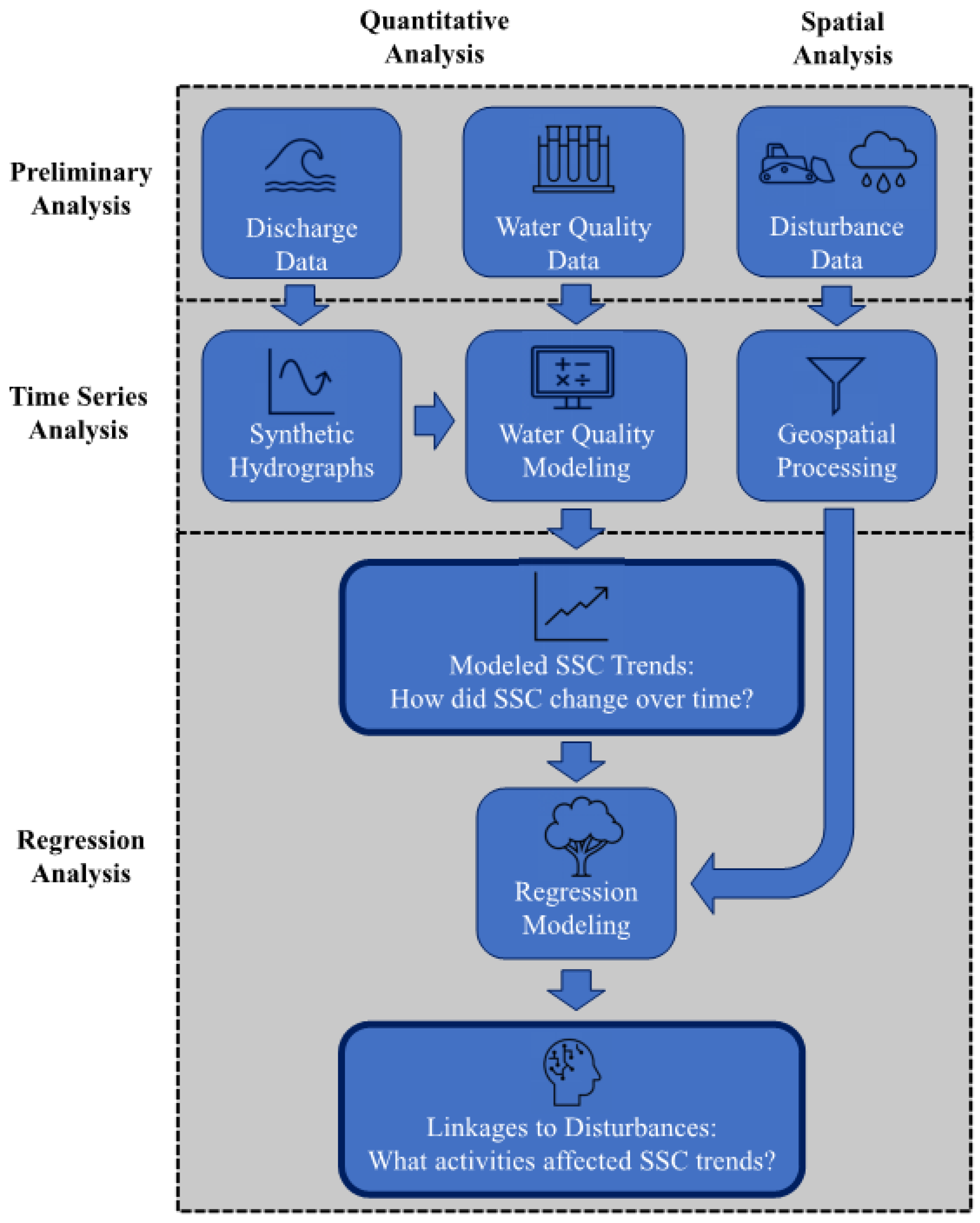
2. Methods

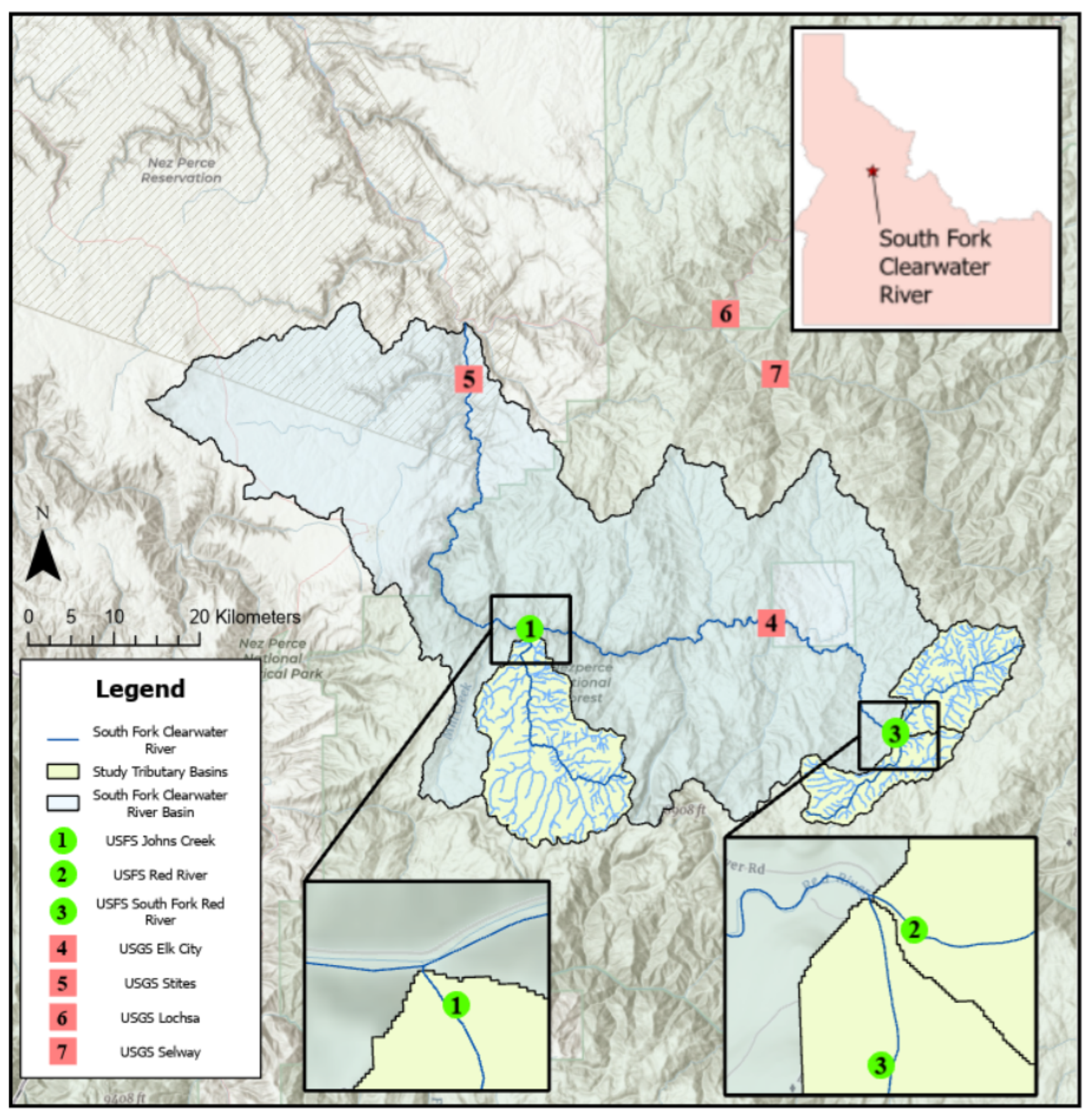
2.1. Study Area

The South Fork Clearwater River (SFCR) drains the western slope of the Bitterroot Mountains that form the border between Montana and Idaho in the interior Pacific Northwest. The SFCR drains a basin of approximately 3043 km² (1175 mi²) [23]. The upper portions of the SFCR watershed (69% of the total land area) are forested land, primarily managed by the United States Forest Service (USFS). Land use in the lower portion of the watershed, the Camas Prairie, is privately owned agricultural (15% of the total land area) and grasslands (7.5% of the total land area). The bottoms reaches and the mouth of the river reside within the Nez Perce Reservation (11% of total land area) [23,24]. Substratum erosion hazard potential ranges from low to high through the landforms in the basin, with the highest potential occurring in the steep, granitic zones and the lowest potential occurring in the flatter, quartzite zones [24]. There are 895 total river kilometers (556 miles) from the headwaters of the SFCR near Elk City, Idaho to the mouth of the Columbia River [25]. As such, this river embodies many of the features characterizing the hydrology of the interior Pacific Northwest, providing a venue for studying several important themes such as legacy anthropogenic environmental degradation, collaborative and multi-objective land management, and tribal sovereignty.

Watershed partners with interest in the SFCR basin include the USFS, the Idaho Department of Environmental Quality (DEQ), recreationalists, private agriculture, and the Nez Perce Tribe (NPT), the latter of which has lived, gathered, hunted, and fished in the SFCR basin and surrounding area since time immemorial [26]. The interest of the USFS is the management of natural resources within the upper basin of the SFCR, which resides within the Nez Perce Clearwater National Forest [27]. The interest of DEQ is the protection of the quality and integrity of Idaho’s natural resources [28]. The interest of the Nez Perce Department of Fisheries Resources Management is the protection of natural resources, treaty rights, and environmental restoration in places have been negatively affected by human impact [26].

Historical resource extraction led to the degradation of water quality in the SFCR and damage to spawning habitat for aquatic species such as the Pacific Lamprey, anadromous salmonids (steelhead, coho, and chinook salmon), and resident salmonids (cutthroat and bull trout), including several species that are listed by the Endangered Species Act (ESA) [23,24,26,29,30]. Among other practices that followed the discovery of gold in the basin in 1861, dredge mining resulted in a dramatic alteration of channel morphologies, the creation of tailings piles along stream banks, and, in some cases, the complete reconfiguration of channel geometry and planform [24]. The construction of roads, harvesting of timber, and grazing of livestock have also had negative impacts on water quality in the basin [24,31,32,33,34,35]. With increased sediment loading to streams, anadromous fish are impacted by suspended sediment in the water and by the deposition of sediment in previously clean gravel beds that prevents spawning [36,37,38,39]. Degraded habitat, reduced water quality, and blocked fish migration (resulting from dams downstream) have all contributed to the observed population of salmonids, both anadromous and resident, being only a small fraction of estimated levels prior to the mid-1800s [24,26], and has triggered violations of the ESA, the Clean Water Act (CWA) [24], and the 1855 and 1863 treaties between the USA and the Nez Perce Tribe, which guarantee the tribe reserved rights to use this river as a usual and accustomed fishery [23,24,26].

In 1998, the state of Idaho listed the SFCR as an impaired body of water per Section 303(d) of the CWA for sediment and temperature [23,24], which prompted a Total Maximum Daily Load (TMDL) for sediment that was published in 2004 in collaboration between the Idaho DEQ, the US Environmental Protection Agency (USEPA), and the Nez Perce Tribe [24]. Between 1998 and 2004, a basin-wide sediment assessment was completed and a sediment loading target was established to limit turbidity to 25 Nephelometric Turbidity Units (NTU) over background conditions for 10 consecutive days, or 50 NTU over background conditions at any time [23]. Background conditions were developed for four control points in the lower basin using stochastic flow modeling and relationships derived from empirical discharge, turbidity, and total suspended solids (TSS) data collected from these four sites. Because no baseline condition estimate was established for much of the upper basin (including the tributary basins Johns Creek, Red River, and South Fork Red River), the TMDL applied the mainstem targeted 25% reduction in sediment yield, which included a margin of safety [23,24]. The TMDL was established for both sediment and temperature impairment; only sediment is considered in the present study. In 2006, an implementation plan was prepared to accomplish the stated goals of the TMDL through a combination of best management practices (BMPs) and restoration activity, such as the reestablishment of floodplains and riparian vegetation to filter runoff. A sediment monitoring plan, included as an appendix to the 2006 TMDL implementation plan, proposed sediment monitoring at three sites throughout the basin but noted that monitoring sediment yield is time- and labor-intensive. Since then, securing the resources required to implement the sediment monitoring plan has proven difficult [23,40]. Accordingly, a renewed effort to establish a sediment monitoring plan has been drafted by an interagency committee led by Idaho DEQ. The focus of this new draft sediment monitoring plan includes assessment of sediment impact on aquatic species, sediment impact of permitted dredge mining, and subbasin sediment priority rankings [41].

The need for improved understanding of sediment loading in the SFCR basin, including establishment of the TMDL, is well documented [23,24,40,42]. This is a challenge for several reasons. Sediment production and availability is complex, difficult to generalize, and varies markedly even in adjacent basins and subbasins [7,43,44]. Additionally, the relationship between basin disturbances and stream characteristics is complex, further obscuring informed decision making by land managers and watershed partners [4,45,46,47,48,49]. Collecting and analyzing sediment samples is resource intensive, so using water quality modeling to augment sample collection to minimize sampling frequency is an enticing strategy for managers [40,50,51,52]. This is the context in which the current study aims to contribute.

2.2. Data Accessed

Over a period of 26 years, starting in water year 1986 and ending in water year 2011 (i.e., 1 October 1985 to 30 September 2011), the USFS collected data from three gauging sites in tributary basins of the SFCR. Moving upstream, these sites are Johns Creek, Red River, and South Fork Red River (Figure 1). At each site, samples were collected via an automated sampler (ISCO Model 1680 Wastewater Sampler, Instrumentation Specialties Company, Lincoln, NE, USA) and analyzed for suspended sediment concentration (SSC) and turbidity according to then-current USFS methods [53]. SSC and turbidity sampling were conducted seasonally at all sites, from approximately May through September. Sampling frequency was sporadic and intermittent, ranging from periods of daily observations to single observations per month. Discharge estimation methods are not well documented for the SFCR but are presumed to have been conducted using traditional methods [54], such as calculation of discharge by multiplying a surveyed cross-sectional area by measured flow velocity. These discharge calculations were then used by the USFS to create rating curves that were updated sporadically throughout the period of record. Stage was typically measured by means of automated bubbler systems. The methods used for creating and maintaining rating curves at the SFCR gaging sites are not well documented. Discharge measurements from Johns Creek, the most downstream of the three gauging stations, were conducted nearly year-round. At Red River and South Fork Red River, discharge measurements were conducted seasonally, from approximately May through September. Details on collection methods, quality assurance, and laboratory procedures are mostly unavailable. Gaps in data collection occurred intermittently at all three sites. Basin area and collection periods are presented in

Table 1. Basin area and collection periods.

Tributary Basin	Area (km2) 1	Area (mi2) 1	SSC Collection (Water Years)	Turbidity Collection (Water Years)
Johns Creek	293	113	1986–2011	1993–2011
Red River	192	74	1986–2010	1993–2010
South Fork Red River	99	38	1995–2010	1995–2010

¹ Source: (USGS, 2019).

. These data were reviewed and compiled into input files for analysis in the statistical software R [55]. Inspection of the data revealed suspected errors that may have occurred during the data entry process, as addressed below in the Discussion.

2.3. Estimation of Missing Discharge Data

The data collected by the USFS at the Johns Creek, Red River, and South Fork Red River gaging stations were only collected seasonally. A complete record of daily discharge is required for the statistical water quality model (introduced in Section 2.4 below), so the following technique was used to estimate the missing discharge data. Further downstream, the USGS maintains gaging sites with measured daily discharge for water years 1986 through 2011 [56]. Using data from the downstream gages as an index, record extensions for the upstream gages were completed by the Maintenance of Variance Extension Type 1 (MOVE.1) index/partial record station regression technique [57,58]. The method develops unbiased record extensions that preserve the mean and variance of low flow estimates by constraining the least ordinary squares regression so that the mean and variance of estimated and observed flows must be equal [57,59]. The MOVE.1 regression equation is $\mathrm{ŷ}\left(i\right)=m\left(y\right)+{\displaystyle \frac{S_y}{S_x}}\left[x\left(i\right)-m\left(x\right)\right]$, where ŷ is the predicted discharge at the partial record site, S is standard deviation, and m is the mean of log-transformed partial record (y) and index (x) flows. This procedure was completed using the Streamflow Record Extension Facilitator (SREF) software [60].

Regressions were developed for three nearby USGS gaging sites, namely Stites (13338500), Lochsa (13337000), and Selway (13336500) (Figure 1), and model goodness-of-fit was compared. The gage at Stites was selected due to presenting more similar hydrologic conditions to the USFS gaging stations than either of the gages at Lochsa or Selway, though all three sites produced acceptable model fits. Synthetic daily discharge records were assembled by filling gaps in the observed data with estimated discharge from the Stites MOVE.1 regressions. These synthetic hydrographs were then input into the water quality model to estimate SSC between observations and develop trends.

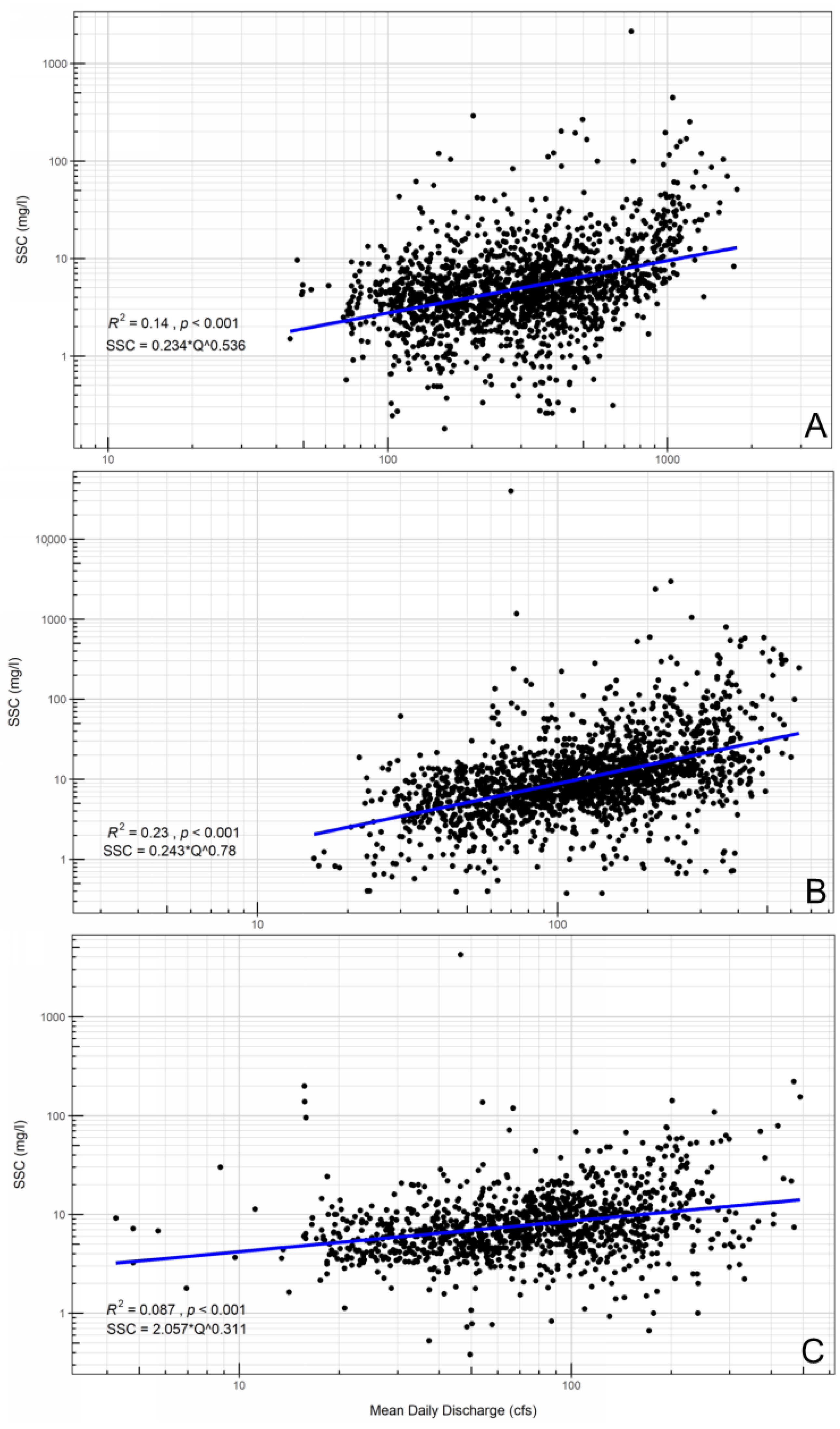
2.4. Modeling Trends in SSC

Modeled trends in water quality and a thorough record of disturbances in the basin can be utilized by land managers and watershed partners to bolster their understanding of the basin and guide informed decision making about how to best utilize future improvement efforts. A statistical water quality modeling approach was chosen for this study over a physical mechanistic modeling approach based on the type of data available in these basins. The data required to run a physical mechanistic model is simply not available at this scale in these basins.

Preliminary analysis of trends in SSC included plotting data distributions and ordinary least squares regression. Because observed SSC varies by orders of magnitude, the least squares regression was performed on ln(SSC) versus ln(discharge), which is equivalent to power law regression. A limitation of this preliminary analysis is the assumption of a constant relationship between discharge and SSC, which is problematic when basin disturbances are ongoing.

To address this limitation, several models have been developed in recent years that can be used to produce normalized sediment load estimates and trends [61,62,63]. One prominent model is the Weighted Regressions on Time, Discharge, and Season (WRTDS) model, a weighted regression algorithm that provides a flexible and robust means of estimating trends in water quality constituents over time [64,65,66,67,68]. WRTDS was chosen for this study because of its flexibility, its ability to work with datasets provided by the USFS, and its robustness—that is, its ability to produce results that are less biased by the natural variability in discharge, seasonality, and changing trends than a simple statistical analysis [65]. Importantly, WRTDS makes no assumption of a constant discharge–SSC relationship, which is critical for identifying whether SSC trends were impacted by factors other than discharge. WRTDS generates estimates of SSC by daily recalibration of predictor variables that are most relevant to each day in the period of record, effectively addressing homoscedastic residuals.

Required inputs for WRTDS are a complete daily discharge record as well as observations of constituents, though the latter does not need to be a complete daily record. Estimates were constructed by the consideration of four factors: three deterministic factors (trend, season, and discharge) and a randomness component [65]. The WRTDS regression equation is $\mathrm{l}n\left(c\right)={\beta }_0+{\beta }_{1}t+{\beta }_2\ln \left(Q\right)+{\beta }_3\sin \left(2\pi t\right)+{\beta }_4\cos \left(2\pi t\right)+\epsilon$, where c is concentration, values of β are fitted model coefficients, discharge is Q, t is the time in years, and unexplained variation is ε. WRTDS was implemented using the Exploration and Graphics for RivEr Trends (EGRET) R package v3.0.7 [66], which produced both flow normalized and non-flow normalized daily estimates of SSC.

Flow normalization accounts for the role of natural variation of daily discharge on water quality. This process is conducted within WRTDS by calculating an estimated concentration for a given day (example: 12 April 1986) with the mean of the daily discharge for that calendar date (12 April) for every year in the period of record (water years 1986–2011). Non-flow normalized estimates of SSC are calculated for a given date without averaging over multiple years. Flow normalization should be utilized when there is a reasonable probability that the distribution of daily discharge has changed in a substantial way across the period of record [65]. While there was no clear indication of changing discharge distribution for these data, both methods (flow normalized and non-flow normalized) were utilized to produce estimates for the purpose of investigation and comparison. Calibration of the WRTDS model was performed by the standard procedure for adjusting weighting parameters (half window widths) [65]. The resulting estimates of SSC from the WRTDS model could then be compared to a record of disturbances in the gauged basins.

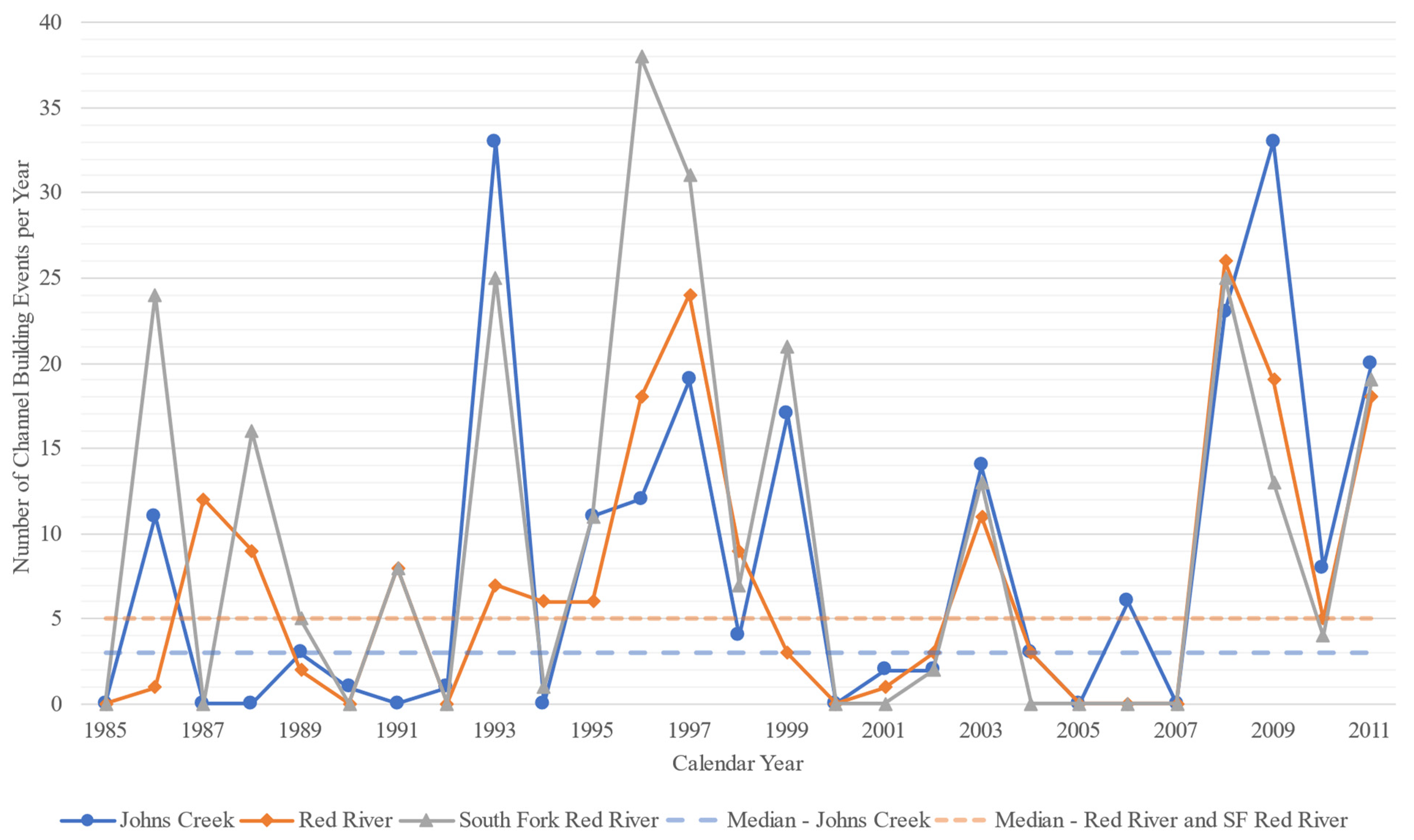
2.5. Basin Disturbance Records

Basin disturbance refers to the collection of natural factors (channel-building flow events) and anthropogenic factors (timber harvesting, hazardous fuel management, controlled burns, and wildfire) that could potentially impact SSC. To develop a record of disturbances in the basin, a dataset was constructed using geospatial land management records provided by the USFS and an annual timeseries of channel-building flow events in each subbasin, referred to hereafter as natural disturbances. Land management records were filtered spatially to the Johns Creek, Red River, and South Fork Red River basins and temporally to include only the years in which water quality samples had been collected at each gaging site. This filtering procedure was conducted in ArcGIS Pro [69]. The date of project completion, activity descriptions, and project acreage were included in the land management record. No data were available regarding project duration, best management practices (BMPs), or other mitigation efforts. Lacking data on project duration, all land management data were aggregated into annual acreage totals by activity type and attributed to the calendar year in which the project was completed. Wildfire is included as an anthropogenic disturbance because no data are available as to the cause or severity of these limited events, so an assumption was made based on location and timing of the few events that occurred during the period of record.

Because land management records were annually aggregated, and because the impact on sediment loading was assumed to not be fully actualized at the mouths of the basins (where the gages are) until the following runoff season, a one-year time lag was applied to anthropogenic disturbances. Thus, anthropogenic activity is allocated to a certain impact year, one year after the calendar year in which the activity occurred. The one-year time lag was determined by a sensitivity analysis of the time lag in Johns Creek, then applied to the other tributary basins being studied. Natural disturbances, or channel-building flow events, were defined for this study as the number of days per year in which the daily mean discharge exceeded the discharge associated with a 1.5 year recurrence interval (Q_1.5). Events of this frequency have been shown to have the greatest potential for sediment mobilization and transport [70,71,72]. Channel-building events were included in the disturbance dataset as a means of testing the variable importance of the land management activities. Channel-building events were chosen as a measure of natural hydrologic disturbance because discharge at the mouth of the basin integrates numerous basin-scale hydrologic processes, represents flows from both rain events as well as snow melt, and incorporates the impact from legacy tailings piles along the channel banks that are assumed to be a major source of mobilizable sediment in basins such as these across the interior Pacific Northwest that have a legacy of mining activity. Because a Q_1.5 is assumed to be approximately a bankfull condition, exceeding this threshold increases the likelihood of the flows topping the channel banks and eroding the tailings piles. The discharge threshold determined to be the Q_1.5 for each subbasin was determined by a Bulletin 17B frequency analysis [73] performed in the software HEC-SSP [74].

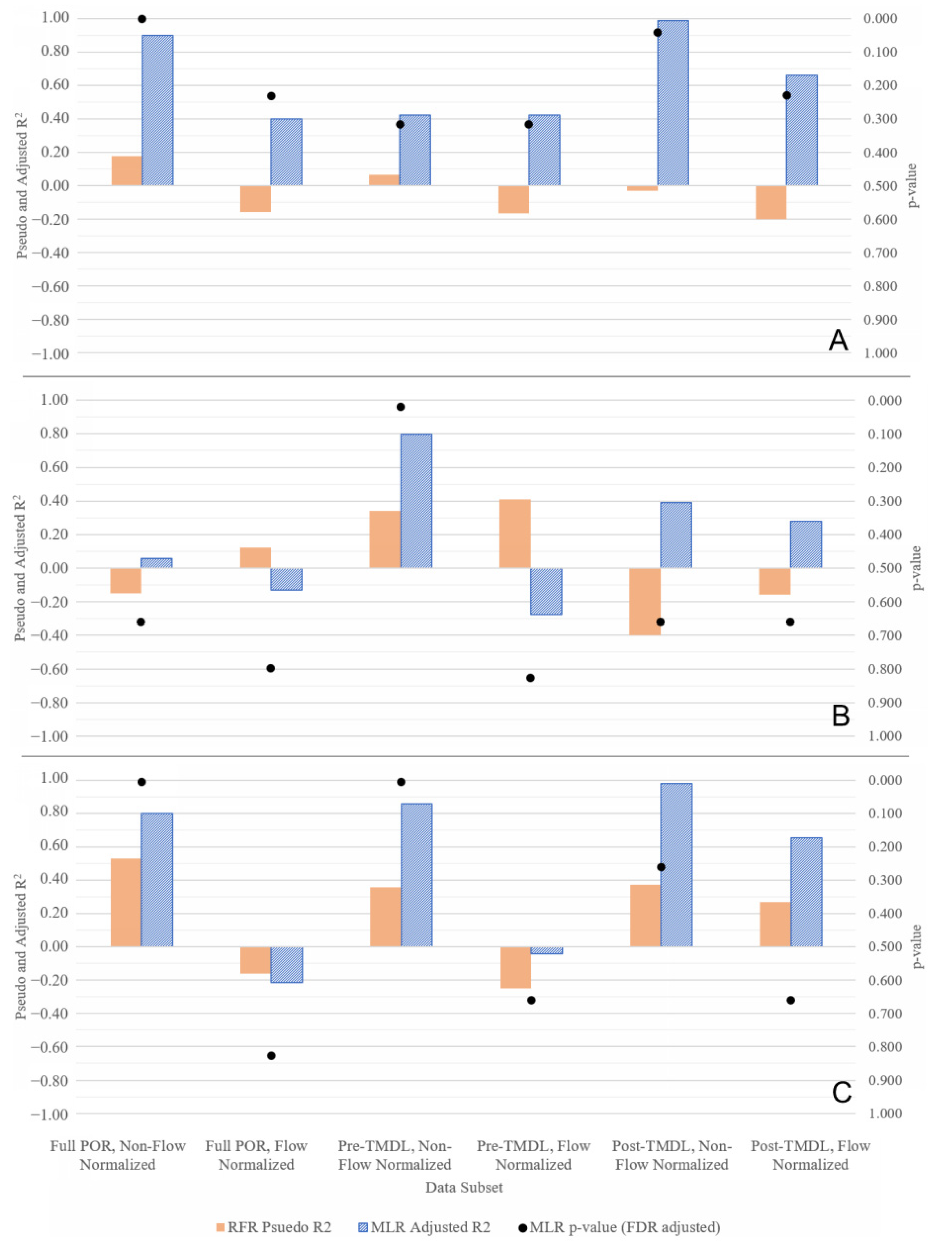
2.6. Testing SSC Trend and Disturbance Relationships with Regression Models

With the modeled trends in SSC and the records of disturbances in each of the tributary basins, we used both multivariable linear regression (MLR) and random forest regression (RFR) to investigate correlations between estimated SSC and both natural disturbances (channel-building events) and anthropogenic land management. MLR fits linear relationships between multiple independent predictor variables and a single dependent outcome variable with the goal of minimizing the sum of the squared differences between predicted and observed results (i.e., ordinary least squares regression). MLR is simple, commonly used, and broadly understood; however, it is not well suited to non-linear and noisy datasets [75,76,77]. MLR models were developed using the lm function from the stats R package [55]. While the SFCR datasets are generally linear, they are noisy. Results of statistical testing of linearity, normality, homoscedasticity, and variable independence of the MLR models were only adequate. For this reason, RFR models were also developed as a supplement to the MLR models because RFR models are better suited to handling noisy datasets.

RFR is a machine learning regression technique comprising an ensemble of non-parametric decision trees used to predict an outcome variable. Bootstrapping is used to randomly select unique subsets of the observed data to train each decision tree in the ensemble (the forest). A number of trees are created in this manner (for this study, n = 10,000). Each decision tree predicts the outcome variable, and the mean of these predictions is the output of the ensemble. This process results in a regression model that can approximately handle non-linearity with no assumption of how the data are distributed. RFR can also quantify individual predictor variable importance relative to the prediction of the dependent outcome variable and has been shown to perform well on SSC datasets when compared to least squares regression [78,79]. RFR models were developed using the randomForest R package v4.7-1.1 [80], and the number of variables evaluated at each split, mtry, was tuned using the tuneRF function from the randomForest package to minimize out-of-bag (OOB) error, the difference between the training values and the values predicted by the model.

The data input to the regression models were the predictor variables (disturbances, both natural and anthropogenic) and the observed outcome variable (WRTDS-modeled SSC). Both types of regression models were run on the entire period of analysis dataset, as well as subsets, to determine the statistical significance of relationships under different scenarios. The first layer of subsets were flow-normalized or non-flow-normalized modeled SSC. Within each of these, further subsets were created for before or after the publication of the TMDL (water years 1986–2004 and 2005–2011, respectively).

Goodness-of-fit for both the MLR and RFR models were compared. For the RFR models, a pseudo R² was evaluated to determine what percentage of the outcome variance was explained by each model, calculated as $Percent Variance Explained=1-{\displaystyle \frac{MS{E}_{OOB}}{{{\widehat{\sigma }}_Y}^2}}$, where $MS{E}_{OOB}$ is the mean of the squared residuals and ${{\widehat{\sigma }}_Y}^2$ is the population variance of the predictions [80]. For RFR models that performed well, individual predictor variable importance was compared. The MLR models were evaluated by adjusted R² to determine what percentage of the outcome variance was explained and p-value to evaluate the statistical significance of the overall model, as well as individual predictor variables. Adjusted R² is determined as the fraction of variance explained by the model, adjusted to only consider predictor variables that improved the model [55].

The analysis in this study was conducted in R (v.4.1.2) and made use of the EGRET R package (v.3.0.7), SREF application (v.1.0), and ArcGIS Pro (v.2.9.1). Input files and scripts used in this analysis are hosted on the findable, accessible, interoperable, and reusable (FAIR) online repository HydroShare (see Data Availability Statement). This HydroShare resource provides the sensitivity analysis to determine the one-year time lag for anthropogenic disturbances, the scripts used to determine regression model goodness-of-fit, and the results discussed below.

3. Results

Following Figure 2, results are broadly categorized into three analysis phases: preliminary, time series, and regression.

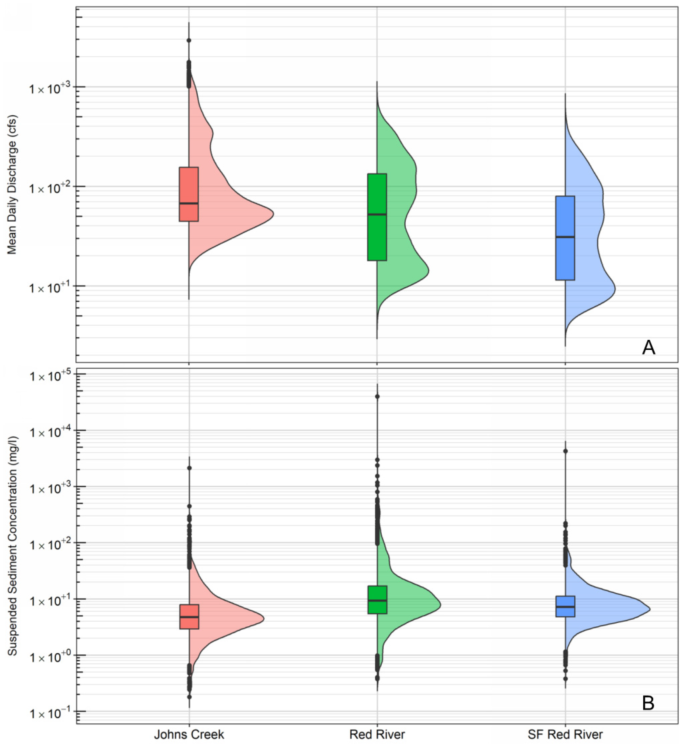
3.1. Preliminary Analysis

Preliminary data analyses included (1) distribution plots of discharge and SSC and (2) ordinary least squares regressions of SSC by discharge. Distribution of the observed discharge and SSC are presented as half-violin plots in Figure 3. At Johns Creek, discharge data were collected nearly year-round, with a median observed discharge of approximately 1.7 m³/s (60 cfs) and a distribution that reflects the flashier nature of the basin and year-round data collection, which skews towards baseflow. At Red River and South Fork Red River, discharge data were only collected seasonally (typically May through September). At Red River, the median observed discharge was approximately 1.4 m³/s (50 cfs), with a distribution that reflects the seasonal data collection, centered around the spring runoff. At South Fork Red River, the median observed discharge was approximately 0.85 m³/s (30 cfs), with a distribution similar to that at Red River.

SSC data were collected seasonally at all three gaging sites. At Johns Creek, the median observed SSC was approximately 5 mg/L. At Red River, the median observed SSC was approximately 10 mg/L. At South Fork Red River, the median observed SSC was approximately 7 mg/L. By visual inspection, the SSC distribution patterns at all three gaging sites were similar and appear to be lognormally distributed.

Functions were fitted using least squares to describe relationships between observed SSC and discharge in Johns Creek, Red River, and South Fork Red River (Figure 4). The percent of variance in SSC explained by these functions was 14%, 23%, and 8.7% at Johns Creek, Red River, and South Fork Red River, respectively. None of these relationships are adequate for prediction or trend analysis because simple statistical methods like power fitting assume a constant relationship between discharge and SSC, which is problematic when basin disturbances are potentially increasing SSC without a change in discharge and making this relationship variable over time. Instead, we proceed to the more sophisticated time series analysis using WRTDS.

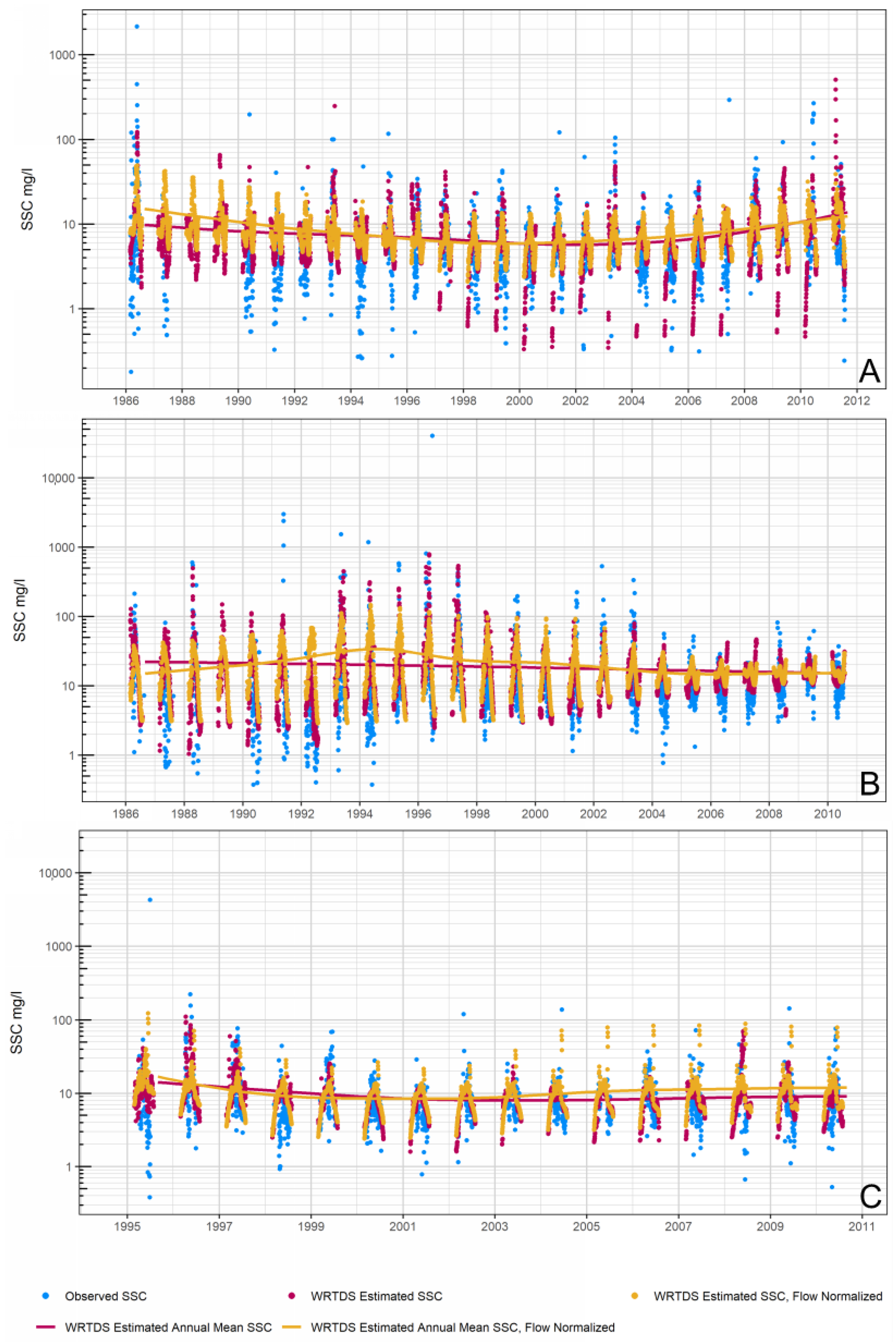
3.2. Time Series Analysis

Model standard error and bias for each tributary are 94.3% standard error and −23% bias at Johns Creek, 114% standard error and −31% bias at Red River, and 75% standard error and −23% bias at South Fork Red River. These model biases are flux biases describing how sediment yield calculated from modeled SSC compared to sediment yield calculated with observed SSC; negative biases indicate that modeled SSC generally underestimated observed SSC. These biases are reasonable for environmental modeling and have been previously observed using WRTDS to model suspended sediment trends in small watersheds with shorter observed records and lower frequency of sampling [81], all of which are the case for the SFCR datasets. The largest flux bias occurs for the Red River basin, where the calculated variance of the observed SSC is much higher than either the Johns Creek or South Fork Red River basins. As shown in Figure 5, WRTDS modeled results, both flow normalized and non-flow normalized, were compared against observed SSC to depict how the ranges of the datasets compared. Flow normalization intends to eliminate the natural variation in SSC due to discharge, which is most evident in unusually wet or dry years. Neither magnitude nor trend in SSC meaningfully changed during the period of record.

3.3. Regression Analysis

Natural and anthropogenic disturbance data are summarized in Figure 6 and Figure 7, respectively. For the MLR and RFR models, the null hypothesis is that the regression slopes are zero. For these models, statistical significance (p-value) and goodness-of-fit metrics that depict how much of the variance in the model estimated SSC was explained by independent predictor variables (adjusted R² for MLR and pseudo R² for RFR) for each model and data subset are presented in Figure 8. Neither model indicates a clear connection between disturbances and sediment concentration trends, which we speculate results from the coarse spatial and temporal scales of the available disturbance data. Investigation of subsets of the data produce some statistically significant relationships between anthropogenic activity and SSC under certain conditions, but the models based on those subsets of the data do not always show agreement regarding goodness-of-fit or variable importance.

The RFR models compared the importance of each predictor variable, that is, how predictive each predictor variable was in the regression analysis. In general, models that evaluated non-flow normalized estimates of SSC indicated that natural predictor variables (channel-building events) were more important than anthropogenic predictor variables. For flow normalized estimates of SSC, anthropogenic predictor variables became more dominant. In other words, flow normalization diminished the relative importance of the hydrologic variables. While some data subsets performed well in both the MLR and RFR models, the models did not always agree on the importance of the same predictor variables.

Although the MLR results are somewhat better than the RFR results, neither approach yielded strong evidence of a correlation in the available data.

4. Discussion

4.1. Data Limitations

This study found no evidence of changing trends in SSC in tributary basins of the SFCR during the period of record. The results additionally suggest that, at the spatial and temporal scale of the available data, the linkages between anthropogenic disturbances in the basin and modeled SSC are unclear, although it should be emphasized that the existence of such linkages cannot be ruled out. This point echoes the finding of Bywater-Reyes et al. [7], who found no evidence for historical activity impacting SSC, which they also attributed to data limitations. More specifically, this finding echoes the conclusion of Edwards et al. [13] that sampling periods exceeding one week were unable to capture sediment transport dynamics. The lack of data, collected at appropriate spatial and temporal scales, also limits the applicability of machine learning.

These results indicate the need for land managers and watershed partners to work towards more directed, collaborative, and impactful management decisions. For a more precise understanding of the sediment regime in these basins, a structured and targeted data collection program should be established using modern methods that include rigorous and thoroughly documented quality control, a focus on finer resolution data collection centered around basin processes and human activities, and a goal of defining baseline sediment concentration and loading in the forested portions of the watershed. The need for such improvements can be demonstrated by looking at the deficiencies of the existing stream data and disturbance records.

The stream data used in this study were collected between water years 1986 and 2011. This period of record is relatively short given basin-scale processes, and with the TMDL established in 2004, provides limited insight into if and how the planned activities set forth in that document affected the sediment regime. Additionally, the collection methods, lab processes, and quality control of the existing stream data are not thoroughly documented. A structured data collection program that is targeted around anthropogenic disturbance activities, such as timber harvest or restoration work, would be required to better understand the impact that these projects are having on the sediment regime in the basin and if the goals set forth by the TMDL are being achieved. With targeted data collection at a finer spatial and temporal scale, along with a rigorous and well-documented quality control program, a more precise understanding of the sediment regime with a higher confidence in results may be achieved using the methods set forth in this study.

Pending availability of resources, future stream data collection strategies should be centered around (1) building and maintaining an understanding of background conditions at basin scale and (2) more precisely targeted monitoring of restoration and disturbance activities. Work is already being done in the basin on the first point, as documented in DEQ [23]. For the second point, the data collection strategy should involve the collection of stream data upstream and downstream of restoration projects or other disturbances before and after the duration of the activity. Downstream monitoring should continue until a baseline post-activity is identified. This will be required to understand the instream impact of specific anthropogenic activities. Data collection should follow established best practices such as those set forth in DEQ [23,41] or from the latest guidance from the USGS. Laboratory analyses of samples should be performed by a qualified laboratory using American Society for Testing Materials (ASTM) method D3977-97 B or similar established best practice. Both collection and analysis practices should be thoroughly documented as metadata alongside stream data, and periodic review should be conducted to ensure the practice is supported by the best available science.

In addition to stream data, more thorough record keeping of land management activity and natural disturbances (namely, mass wasting) would greatly improve the understanding of the natural variance of the sediment regime and the anthropogenic impact on water quality in these basins. For most anthropogenic disturbances, this would include an objective metric of harvest intensity per acre, as well as having project start and end dates associated with geospatial data. Lack of data on roads is a meaningful gap in the land management record for the upper portions of the SFCR basin, including the Johns Creek, Red River, and South Fork Red River tributary basins. While geospatial data are available regarding the existence, location, and geometry of active and decommissioned roads, none of these data have a temporal component that identifies when the road was built, when major maintenance activities associated with the road occurred, or how use of these roads has changed over time. Any of these activities could have resulted in an increase in sediment mobilization to streams, and it is reasonable to assume that roads play a meaningful role in the sediment regime in these basins [31,45,47]. Without these temporal data we cannot identify correlative relationships about how roads and road activity have impacted water quality over time. We hypothesize that this data gap and with the other data limitations identified in this section are contributing factors to model uncertainty and error.

4.2. Model Uncertainties and Error

By necessity, the methods set forth in this study made simplifying assumptions at multiple stages. First, due to data collection being seasonal (i.e., May to September) and gaps in the observed record, it was necessary to simulate certain components of the daily discharge record. Second, the modeled daily discharge records, along with observations in SSC, were input into a water quality model to develop normalized trends in SSC over time. And third, these modeled trends in SSC and records of disturbances were input into regression models to explore correlation between basin disturbances and modeled SSC. At each stage of this process, model uncertainty and error of varying magnitudes were incurred. The largest uncertainty was associated with the water quality modeling. This is reasonable to expect in environmental modeling as these are complex systems that are being simplistically represented in both the data and the models; however, the small sample size, seasonality, data gaps, and unclear data collection/quality control procedures all likely increased model uncertainty and error.

While these limitations bring the accuracy of the magnitudes of the modeled SSC into question, the trends in the modeled results still provide valuable insight into how the basin is changing, or not changing, over time. Model uncertainty and error can be reduced by increasing the number of samples collected over a longer period of time and more frequently [81], though land managers and watershed partners should carefully consider the balance between improving model uncertainty and error and the costs associated with more intensive sampling. Work is being conducted to study how to achieve this balance based on sampling frequency and the accuracy of modeled results [52].

4.3. Intentions and Effectiveness of TMDL in Addressing Legacy Degradation

The TMDL that was established for the SFCR in 2004 set forth a goal for reducing sediment loading that was intended to regulate and reduce new sources of sediment loading to streams in the basin. While such a reduction is critical to preventing future negative impacts on water quality and anadromous fish habitat, it does not address the problem of legacy degradation, including, but not limited to, dredge mining. Historic dredge mining resulted in physical substrate alteration, tailings piles on banks, and, in some cases, completely reconfigured channel morphologies. It is reasonable to assume that all these alterations have the potential to increase sediment loading and therefore to reduce the quality and availability of fish habitat [24,31,32,33,34,35].

To address this legacy damage, an effort to revise the existing implementation plan could be established to target critical restoration efforts with the goal of returning channel, bank, and floodplain conditions to an approximation of their conditions before the mid-1800s. There are projects that have occurred or are underway in the basin since 2011 that have begun this work, notably in the Newsome Creek and Crooked River tributary basins. A renewed effort to establish a monitoring plan was underway as of March 2023 by an interagency committee led by the Idaho DEQ. The focus of this new draft monitoring plan includes assessment of sediment impact on aquatic species, sediment impact of permitted dredge mining, and subbasin sediment priority rankings [41]. To maximize the benefit of the revised sediment monitoring plan, it is recommended that stream data be collected upstream and downstream of a restoration project, timber harvest, or permitted dredge mining activity before, during, and for several years after completion of the project or activity to observe the impact on water quality over time.

5. Conclusions

This work is the first distillation of the SSC data collected in the SFCR over water years 1986–2011 and has been compiled into a HydroShare repository for future use. Analysis of these data show that trends in SSC did not change over the period of record. This study suggests that the available data in the basin are not sufficient for predicting changes in SSC trends and provides a monitoring program design to ensure unambiguous measurements of water quality data to support future management decision making. Using data from the Johns Creek, Red River, and South Fork Red River tributary basins, we have demonstrated the following:

• Sediment concentration trends did not change meaningfully during the period of record, including before and after the establishment of the TMDL in 2004.
• At this spatial and temporal scale, linkages between anthropogenic disturbances and trends in SSC are unclear, though the existence of such linkages cannot be ruled out.

The limitations of this study center primarily on the type, quality, and quantity of available data in the basin. Uncertainties in data collection, laboratory analysis, and quality control methods, combined with infrequent and seasonal sampling frequency, lead to severe challenges in clearly understanding a basin’s sediment regime. Additionally, many natural and anthropogenic factors that are known to impact sediment production and transport, such as mass wasting or road activities, are lacking usable data in this basin for a time series or regression analysis. This is detrimental for developing a predictive model as training data do not include a full picture of basin processes that affect sediment mobilization and transport. To overcome these challenges, we used layers of modeling, each of these contributing towards a cumulative uncertainty in the overall analysis. This can be addressed in future work by the application of a focused and targeted data collection approach with rigorous quality control standards. Future work could also apply the methodology set forth in this study to datasets from additional basins to improve these techniques and further the development of decision support tools for land managers and watershed partners.

Land managers and watershed partners are often faced with the difficult task of deciding how to use limited resources to achieve maximum impact. In the case of the SFCR, extensive legacy environmental degradation has left the basin with persistent water quality concerns that have affected the habitat for listed anadromous fish species and a fishery used by the Nez Perce Tribe since time immemorial. Even with limited datasets of water quality and disturbance records, the methods set forth in this study provide land managers and watershed partners with means to evaluate the impact of anthropogenic activity as well as the effectiveness of regulatory and restoration activities within a given basin. This information can be used by land managers and watershed partners to direct further structured and targeted data collection efforts to improve the precision and robustness of their understanding of the sediment regime in these basins.

References

- Cole, R.P.; Bladon, K.D.; Wagenbrenner, J.W.; Coe, D.B.R. Hillslope Sediment Production after Wildfire and Post-fire Forest Management in Northern California. Hydrol. Process 2020, 34, 5242–5259. [Google Scholar] [CrossRef]
- Dethier, E.N.; Renshaw, C.E.; Magilligan, F.J. Rapid Changes to Global River Suspended Sediment Flux by Humans. Science 2022, 376, 1447–1452. [Google Scholar] [CrossRef] [PubMed]
- Larsen, M.C.; Gellis, A.C.; Glysson, G.D.; Gray, J.R.; Horowitz, A.J. Fluvial Sediment in the Environment: A National Challenge. In Proceedings of the Joint Federal Interagency Conference 2010: Hydrology and Sedimentation for a Changing Future: Existing and Emerging Issues, Las Vegas, Nevada, USA, 27 June–1 July 2010. [Google Scholar]
- Roper, B.; Saunders, W.C.; Ojala, J.V. The Relationship between Disturbance Events and Substantial Changes in Stream Conditions on Public Lands in the Inland Pacific Northwest. N. Am. J. Fish. Manag. 2022, 43, 268–290. [Google Scholar] [CrossRef]
- Bedient, P.B.; Huber, W.C.; Vieux, B.E. Hydrology and Floodplain Analysis, 6th ed.; Pearson: New York, NY, USA, 2019; ISBN 978-0-13-475197-9. [Google Scholar]
- Wainger, L.A. Opportunities for Reducing Total Maximum Daily Load (TMDL) Compliance Costs: Lessons from the Chesapeake Bay. Environ. Sci. Technol. 2012, 46, 9256–9265. [Google Scholar] [CrossRef]
- Bywater-Reyes, S.; Bladon, K.D.; Segura, C. Relative Influence of Landscape Variables and Discharge on Suspended Sediment Yields in Temperate Mountain Catchments. Water Resour. Res. 2018, 54, 5126–5142. [Google Scholar] [CrossRef]
- Liu, Q.J.; Zhang, H.Y.; Gao, K.T.; Xu, B.; Wu, J.Z.; Fang, N.F. Time-Frequency Analysis and Simulation of the Watershed Suspended Sediment Concentration Based on the Hilbert-Huang Transform (HHT) and Artificial Neural Network (ANN) Methods: A Case Study in the Loess Plateau of China. CATENA 2019, 179, 107–118. [Google Scholar] [CrossRef]
- Navratil, O.; Esteves, M.; Legout, C.; Gratiot, N.; Nemery, J.; Willmore, S.; Grangeon, T. Global Uncertainty Analysis of Suspended Sediment Monitoring Using Turbidimeter in a Small Mountainous River Catchment. J. Hydrol. 2011, 398, 246–259. [Google Scholar] [CrossRef]
- Walling, D.E. The Sediment Delivery Problem. J. Hydrol. 1983, 65, 209–237. [Google Scholar] [CrossRef]
- Fryirs, K. (Dis) Connectivity in Catchment Sediment Cascades: A Fresh Look at the Sediment Delivery Problem. Earth Surf. Process Landf. 2013, 38, 30–46. [Google Scholar] [CrossRef]
- McEachran, Z.P.; Karwan, D.L.; Slesak, R.A. Direct and Indirect Effects of Forest Harvesting on Sediment Yield in Forested Watersheds of the United States. J. Am. Water Resour. Assoc. 2021, 57, 1–31. [Google Scholar] [CrossRef]
- Edwards, P.J.; Williard, K.W.J.; Kochenderfer, J.N. Sampling Considerations for Establishment of Baseline Loadings from Forested Watersheds for TMDL Application. Env. Monit. Assess. 2004, 98, 201–223. [Google Scholar] [CrossRef] [PubMed]
- Ouyang, Y. A Gap-Filling Tool: Predicting Daily Sediment Loads Based on Sparse Measurements. Hydrology 2022, 9, 181. [Google Scholar] [CrossRef]
- Davis, C.M.; Fox, J.F. Sediment Fingerprinting: Review of the Method and Future Improvements for Allocating Nonpoint Source Pollution. J. Environ. Eng. 2009, 135, 490–504. [Google Scholar] [CrossRef]
- Mukundan, R.; Walling, D.E.; Gellis, A.C.; Slattery, M.C.; Radcliffe, D.E. Sediment Source Fingerprinting: Transforming From a Research Tool to a Management Tool. J. Am. Water Resour. Assoc. 2012, 48, 1241–1257. [Google Scholar] [CrossRef]
- Voli, M.T.; Wegmann, K.W.; Bohnenstiehl, D.R.; Leithold, E.; Osburn, C.L.; Polyakov, V. Fingerprinting the Sources of Suspended Sediment Delivery to a Large Municipal Drinking Water Reservoir: Falls Lake, Neuse River, North Carolina, USA. J. Soils Sediments 2013, 13, 1692–1707. [Google Scholar] [CrossRef]
- Shah, N.W.; Baillie, B.R.; Bishop, K.; Ferraz, S.; Högbom, L.; Nettles, J. The Effects of Forest Management on Water Quality. For. Ecol. Manag. 2022, 522, 120397. [Google Scholar] [CrossRef]
- Klein, R.D.; Lewis, J.; Buffleben, M.S. Logging and Turbidity in the Coastal Watersheds of Northern California. Geomorphology 2012, 139–140, 136–144. [Google Scholar] [CrossRef]
- Witt, E.L.; Barton, C.D.; Stringer, J.W.; Kolka, R.K.; Cherry, M.A. Influence of Variable Streamside Management Zone Configurations on Water Quality after Forest Harvest. J. For. 2016, 114, 41–51. [Google Scholar] [CrossRef]
- Karwan, D.L.; Gravelle, J.A.; Hubbart, J.A. Effects of Timber Harvest on Suspended Sediment Loads in Mica Creek, Idaho. For. Sci. 2007, 53, 181–188. [Google Scholar] [CrossRef]
- López-Tarazón, J.A.; Estrany, J. Exploring Suspended Sediment Delivery Dynamics of Two Mediterranean Nested Catchments. Hydrol. Process 2017, 31, 698–715. [Google Scholar] [CrossRef]
- Idaho Department of Environmental Quality. Suspended Sediment Patterns in the South Fork Clearwater River and Selected Tributaries; Idaho Department of Environmental Quality: Boise, ID, USA, 2022. [Google Scholar]
- Idaho Department of Environmental Quality, Nez Perce Tribe. South Fork Clearwater River Subbasin Assessment and Total Maximum Daily Loads; U.S. Environmental Protection Agency: Boise, ID, USA, 2004. [Google Scholar]
- U.S. Geological Survey USGS|Streamer. Available online: https://webapps.usgs.gov/streamer/ (accessed on 25 March 2023).
- Nez Perce Tribe Department of Fisheries Resources Management. Management Plan; Nez Perce Tribe: Boise, ID, USA, 2013. [Google Scholar]
- U.S. Forest Service. This Is Who We Are; U.S. Forest Service: Washington, DC, USA, 2019. [Google Scholar]
- Idaho Department of Environmental Quality. About Us; Idaho Department of Environmental Quality: Boise, ID, USA, 2023. [Google Scholar]
- National Oceanic and Atmospheric Administration (NOAA) Fisheries. Endangered Species Act Section 7(a)(2) Consultation Biological Opinion And Magnuson-Stevens Fishery Conservation and Management Act Essential Fish Habitat Consultation; NOAA: Silver Spring, MD, USA, 2008. [Google Scholar]
- U.S. Forest Service. Aquatic Evaluation Report, Federally Listed Species, Species-of-Concern and Species-of-Interest, Nez Perce National Forest; U.S. Forest Service: Washington, DC, USA, 2015. [Google Scholar]
- Anderson, P.G. Sediment Generation from Forestry Operations and Associated Effects on Aquatic Ecosystems. In Proceedings of the Forest-Fish Conference: Land Management Practices Affecting Aquatic Ecosystems, Calgary, AB, Canada, 1–4 May 1996. [Google Scholar]
- Bash, J.; Berman, C.H.; Bolton, S. Effects of Turbidity and Suspended Solids on Salmonids; University of Washington Water Center: Seattle, WA, USA, 2001. [Google Scholar]
- Orndorff, A. Evaluating the Effects of Sedimentation from Forest Roads; University of Florida: Gainesville, FL, USA, 2017. [Google Scholar]
- Quigley, J.T. Experimental Field Manipulation of Stream Temperatures and Suspended Sediment Concentrations: Behavioural and Physiological Effects to Juvenile Chinook Salmon. Ph.D. Thesis, University of British Columbia, Vancouver, BC, Canada, 2009. [Google Scholar] [CrossRef]
- Wenger, A.S.; Harvey, E.; Wilson, S.; Rawson, C.; Newman, S.J.; Clarke, D.; Saunders, B.J.; Browne, N.; Travers, M.J.; Mcilwain, J.L.; et al. A Critical Analysis of the Direct Effects of Dredging on Fish. Fish. 2017, 18, 967–985. [Google Scholar] [CrossRef]
- Berli, B.I.; Gilbert, M.J.H.; Ralph, A.L.; Tierney, K.B.; Burkhardt-Holm, P. Acute Exposure to a Common Suspended Sediment Affects the Swimming Performance and Physiology of Juvenile Salmonids. Comp. Biochem. Physiol. Part A Mol. Integr. Physiol. 2014, 176, 1–10. [Google Scholar] [CrossRef] [PubMed]
- Harvey, B.C.; Lisle, T.E. Effects of Suction Dredging on Streams: A Review and an Evaluation Strategy. Fisheries 1998, 23, 8–17. [Google Scholar] [CrossRef]
- Jensen, D.W.; Steel, E.A.; Fullerton, A.H.; Pess, G.R. Impact of Fine Sediment on Egg-To-Fry Survival of Pacific Salmon: A Meta-Analysis of Published Studies. Rev. Fish. Sci. 2009, 17, 348–359. [Google Scholar] [CrossRef]
- Platts, W.S.; Torquemada, R.J.; McHenry, M.L.; Graham, C.K. Changes in Salmon Spawning and Rearing Habitat from Increased Delivery of Fine Sediment to the South Fork Salmon River, Idaho. Trans. Am. Fish. Soc. 1989, 118, 274–283. [Google Scholar] [CrossRef]
- South Fork Clearwater River Watershed Advisory Group. South Fork Clearwater River TMDL Implementation Plan. 2006. Available online: https://www2.deq.idaho.gov/admin/LEIA/api/document/download/11781 (accessed on 25 February 2025).
- Idaho Department of Environmental Quality. South Fork Clearwater River Sediment Assessment Plan (2023–2027) Version 1.0; Idaho Department of Environmental Quality: Boise, ID, USA, 2023. [Google Scholar]
- Thomas, R.; King, J.G. Sediment Yield and Model Test in Main and South Forks of Red River Water Years 1986–2011. A Report Submitted to the US Department of Agriculture, Forest Service, Boise Adjudication Team and the Nez Perce National Forest; Hydrology Consulting: Boise, ID, USA, 2004. [Google Scholar]
- Goodman, A.C.; Segura, C.; Jones, J.A.; Swanson, F.J. Seventy Years of Watershed Response to Floods and Changing Forestry Practices in Western Oregon, USA. Earth Surf. Process Landf. 2023, 48, 1103–1118. [Google Scholar] [CrossRef]
- Ryan, S.E.; Dixon, M.K. Spatial and Temporal Variability in Stream Sediment Loads Using Examples from the Gros Ventre Range, Wyoming, USA. In Gravel Bed Rivers VI: From Process Understanding to River Restoration. Developments in Earth Surface Processes; Habersack, H., Piegay, H., Rinaldi, M., Eds.; Elsevier: Amsterdam, The Netherlands, 2007; Volume 11, pp. 387–407. [Google Scholar]
- Al-Chokhachy, R.; Black, T.A.; Thomas, C.; Luce, C.H.; Rieman, B.; Cissel, R.; Carlson, A.; Hendrickson, S.; Archer, E.K.; Kershner, J.L. Linkages between Unpaved Forest Roads and Streambed Sediment: Why Context Matters in Directing Road Restoration. Restor. Ecol. 2016, 24, 589–598. [Google Scholar] [CrossRef]
- Bywater-Reyes, S.; Segura, C.; Bladon, K.D. Geology and Geomorphology Control Suspended Sediment Yield and Modulate Increases Following Timber Harvest in Temperate Headwater Streams. J. Hydrol. 2017, 548, 754–769. [Google Scholar] [CrossRef]
- Elliot, W.J.; Page-Dumroese, D.; Robichaud, P.R. The Effects of Forest Management on Erosion and Soil Productivity. In Soil Quality and Soil Erosion; Lal, R., Ed.; CRC Press: Boca Raton, FL, USA, 2018; pp. 195–208. ISBN 978-0-203-73926-6. [Google Scholar]
- Hunsaker, C.T.; Neary, D.G. Sediment Loads and Erosion in Forest Headwater Streams of the Sierra Nevada, California. In Revisiting Experimental Catchment Studies in Forest Hydrology: Proceedings of a Workshop Held During the XXV IUGG General Assembly in Melbourne, June–July 2011; Webb, A.A., Bonell, M., Bren, L., Lane, P.N.J., McGuire, D., Neary, D.G., Nettles, J., Scott, D.F., Stednik, J., Wang, Y., Eds.; Wallingford: International Association of Hydrological Sciences; IAHS Publication 353: Wallingford, UK, 2012; pp. 195–204. [Google Scholar]
- Safeeq, M.; Grant, G.E.; Lewis, S.L.; Hayes, S.K. Disentangling Effects of Forest Harvest on Long-Term Hydrologic and Sediment Dynamics, Western Cascades, Oregon. J. Hydrol. 2020, 580, 124259. [Google Scholar] [CrossRef]
- Cheviron, B.; Delmas, M.; Cerdan, O.; Mouchel, J.-M. Calculation of River Sediment Fluxes from Uncertain and Infrequent Measurements. J. Hydrol. 2014, 508, 364–373. [Google Scholar] [CrossRef]
- Srivastava, A.; Brooks, E.S.; Dobre, M.; Elliot, W.J.; Wu, J.Q.; Flanagan, D.C.; Gravelle, J.A.; Link, T.E. Modeling Forest Management Effects on Water and Sediment Yield from Nested, Paired Watersheds in the Interior Pacific Northwest, USA Using WEPP. Sci. Total Environ. 2020, 701, 134877. [Google Scholar] [CrossRef]
- Yoder, A. High Frequency Total Phosphorus Observations from the Lower Boise River. In Proceedings of the IDEQ Water Quality Workshop 2022, Boise, ID, USA, 16–17 March 2022. [Google Scholar]
- Thomas, R.B. Measuring Suspended Sediment in Small Mountain Streams; Department of Agriculture, Forest Service, Pacific Southwest Forest and Range Experiment Station: Berkeley, CA, USA, 1985; Volume 9, p. 83. [Google Scholar] [CrossRef]
- U.S. Geological Survey. Measurement and Computation of Streamflow; U.S. Geological Survey: Reston, VA, USA, 1982. [Google Scholar]
- R Core Team. R: A Language and Environment for Statistical Computing; R Foundation for Statistical Computing: Vienna, Austria, 2021; Available online: https://www.R-project.org/ (accessed on 25 February 2025).
- U.S. Geological Survey. SF Clearwater River at Stites ID. Available online: https://waterdata.usgs.gov/monitoring-location/13338500/ (accessed on 25 March 2023).
- Colarullo, S.J.; Sullivan, S.L.; McHugh, A.R. Implementation of MOVE.1, Censored MOVE.1, and Piecewise MOVE.1 Low-Flow Regressions with Applications at Partial-Record Streamgaging Stations in New Jersey; U.S. Geological Survey: Reston, VA, USA, 2018. [Google Scholar]
- Hirsch, R.M. A Comparison of Four Streamflow Record Extension Techniques. Water Resour. Res. 1982, 18, 1081–1088. [Google Scholar] [CrossRef]
- Clark, G.M.; Ducar, S.D. Sediment Transport in the Yankee Fork of the Salmon River Near Stanley, Idaho, Water Years 2012–2019; U.S. Geological Survey: Reston, VA, USA, 2021. [Google Scholar]
- Granato, G.E. Computer Programs for Obtaining and Analyzing Daily Mean Streamflow Data from the U.S. Geological Survey National Water Information System Web Site. Appendix 3. Streamflow Record Extension Facilitator (SREF Version 1.0)—A Program for Extending and Augmenting Available Streamflow Data Using Long-Term Streamflow Records from Hydrologically Similar Sites; Open-File Report; U.S. Geological Survey: Reston, VA, USA, 2009. [Google Scholar]
- Appling, A.P.; Leon, M.C.; McDowell, W.H. Reducing Bias and Quantifying Uncertainty in Watershed Flux Estimates: The R Package Loadflex. Ecosphere 2015, 6, 1–25. [Google Scholar] [CrossRef]
- Hirsch, R.M.; Archfield, S.A.; De Cicco, L.A. A Bootstrap Method for Estimating Uncertainty of Water Quality Trends. Environ. Model. Softw. 2015, 73, 148–166. [Google Scholar] [CrossRef]
- Lee, C.J.; Hirsch, R.M.; Schwarz, G.E.; Holtschlag, D.J.; Preston, S.D.; Crawford, C.G.; Vecchia, A.V. An Evaluation of Methods for Estimating Decadal Stream Loads. J. Hydrol. 2016, 542, 185–203. [Google Scholar] [CrossRef]
- Goswami, A.; Paul, P.K.; Rudra, R.; Goel, P.K.; Daggupati, P. Evaluation of Statistical Models: Perspective of Water Quality Load Estimation. J. Hydrol. 2023, 616, 128721. [Google Scholar] [CrossRef]
- Hirsch, R.M.; Moyer, D.L.; Archfield, S.A. Weighted Regressions on Time, Discharge, and Season (WRTDS), with an Application to Chesapeake Bay River Inputs. J. Am. Water Resour. Assoc. 2010, 46, 857–880. [Google Scholar] [CrossRef]
- Hirsch, R.M.; De Cicco, L.A. User Guide to Exploration and Graphics for RivEr Trends (EGRET) and dataRetrieval: R Packages for Hydrologic Data; Techniques and Methods; Version 1.0: Originally posted 8 October 2014; Version 2.0: 5 February 2015; U.S. Geological Survey: Reston, VA, USA, 2015; p. 104. [Google Scholar]
- Oelsner, G.P.; Sprague, L.A.; Murphy, J.C.; Zuellig, R.E.; Johnson, H.M.; Ryberg, K.R.; Falcone, J.A.; Stets, E.G.; Vecchia, A.V.; Riskin, M.L.; et al. Water-Quality Trends in the Nation’s Rivers and Streams, 1972–2012—Data Preparation, Statistical Methods, and Trend Results; Scientific Investigations Report; Version 1.0: Originally posted 4 April 2017; Version 2.0: 1 November 2017; U.S. Geological Survey: Reston, VA, USA, 2017; p. 158. [Google Scholar]
- Zhang, Q.; Hirsch, R.M. River Water-Quality Concentration and Flux Estimation Can Be Improved by Accounting for Serial Correlation Through an Autoregressive Model. Water Resour. Res. 2019, 55, 9705–9723. [Google Scholar] [CrossRef]
- Esri Inc. ArcGIS Pro; Esri Inc.: Redlands, CA, USA, 2022. [Google Scholar]
- Leopold, L.B.; Wolman, M.G.; Miller, J.P.; Wohl, E.E. Fluvial Processes in Geomorphology; Dover, Ed.; Dover Publications, Inc.: Mineola, NY, USA, 2020; ISBN 978-0-486-84552-4. [Google Scholar]
- Ward, A.; Moran, M. A Novel Approach for Estimating the Recurrence Intervals of Channel-Forming Discharges. Water 2016, 8, 269. [Google Scholar] [CrossRef]
- Wolman, M.G.; Miller, J.P. Magnitude and Frequency of Forces in Geomorphic Processes. J. Geol. 1960, 68, 54–74. [Google Scholar] [CrossRef]
- U.S. Water Resources Council. Guidelines for Determining Flood Flow Frequency, Bulletin No. 17B; U.S. Water Resources Council, Subcommittee on Hydrology: Washington, DC, USA, 1982. [Google Scholar]
- Hydrologic Engineering Center. HEC-SSP; Hydrologic Engineering Center: Davis, CA, USA, 2023. [Google Scholar]
- Adamowski, J.; Karapataki, C. Comparison of Multivariate Regression and Artificial Neural Networks for Peak Urban Water-Demand Forecasting: Evaluation of Different ANN Learning Algorithms. J. Hydrol. Eng. 2010, 15, 729–743. [Google Scholar] [CrossRef]
- Smith, P.F.; Ganesh, S.; Liu, P. A Comparison of Random Forest Regression and Multiple Linear Regression for Prediction in Neuroscience. J. Neurosci. Methods 2013, 220, 85–91. [Google Scholar] [CrossRef]
- Zounemat-Kermani, M.; Kişi, Ö.; Adamowski, J.; Ramezani-Charmahineh, A. Evaluation of Data Driven Models for River Suspended Sediment Concentration Modeling. J. Hydrol. 2016, 535, 457–472. [Google Scholar] [CrossRef]
- Breiman, L. Random Forests. Mach. Learn. 2001, 45, 5–32. [Google Scholar] [CrossRef]
- Francke, T.; López-Tarazón, J.A.; Schröder, B. Estimation of Suspended Sediment Concentration and Yield Using Linear Models, Random Forests and Quantile Regression Forests. Hydrol. Process 2008, 22, 4892–4904. [Google Scholar] [CrossRef]
- Liaw, A.; Wiener, M. Classification and Regression by randomForest. R News. 2002, 2/3, 18–22. [Google Scholar]
- Zhang, Q.; Blomquist, J.D.; Moyer, D.L.; Chanat, J.G. Estimation Bias in Water-Quality Constituent Concentrations and Fluxes: A Synthesis for Chesapeake Bay Rivers and Streams. Front. Ecol. Evol. 2019, 7, 109. [Google Scholar] [CrossRef]