Article

TopEros: An Integrated Hydrology and Multi-Process Erosion Model—A Comparison with MUSLE

1
Centre for Climate Change Adaptation, National Institute for Environmental Studies, Tsukuba 305-8506, Japan
2
Graduate School of Agricultural and Life Sciences, The University of Tokyo, Tokyo 113-8657, Japan
3
Faculty of Applied Biological Sciences, Gifu University, Gifu 501-1193, Japan
4
NTC-International Co., Ltd., Tokyo 136-0071, Japan
*
Author to whom correspondence should be addressed.
Hydrology 2025, 12(11), 309; https://doi.org/10.3390/hydrology12110309
Submission received: 22 September 2025 / Revised: 13 November 2025 / Accepted: 15 November 2025 / Published: 20 November 2025

Abstract

Hydro-erosion is a primary driver of soil degradation worldwide, yet accurate catchment-scale prediction remains challenging because sheet, gully, and raindrop-impact detachment processes operate simultaneously at sub-grid scales. We introduce TopEros, a hydro-erosion model that integrates the hydrological framework of TOPMODEL with three distinct erosion modules: sheet erosion, gully erosion, and raindrop-impact detachment. TopEros employs a sub-grid zoning strategy in which each grid cell is partitioned into diffuse-flow (sheet erosion) and concentrated-flow (gully erosion) domains using threshold values of two topographic indices: the topographic index (TI) and the contributing area–slope index (aitanβ). Applied to the Namatala River catchment in eastern Uganda and calibrated with TI = 15 and aitanβ = 35, TopEros identified sheet-dominated and gully-prone areas. The simulated specific sediment yields ranged from 95 to 155 Mgha−1yr−1—classified as “high” to “very high”—with gully zones contributing disproportionately large erosion volumes. These results demonstrate the importance of capturing intra-cell heterogeneity: conventional catchment-average approaches can obscure critical erosion hotspots. By explicitly representing multiple soil detachment and transport mechanisms within a unified process-based framework, TopEros has the potential to enhance the realism of catchment-scale erosion estimates and support the precise targeting of soil and water conservation measures.

1. Introduction

Soil erosion by water is a pervasive hydrological phenomenon and remains a dominant driver of soil degradation globally [1]. The accelerated loss of fertile topsoil lowers agricultural productivity and heightens reservoir siltation and degradation of water quality [2]. Hydro-erosion involves several mechanisms: detachment by diffuse flow (sheet and inter-rill erosion), detachment by concentrated flow (rill and gully erosion), and detachment of particles by raindrop impact. Notably, although gullies typically occupy a limited portion of the landscape, they can dominate sediment export from a catchment: often contributing from 10 to 95% of the total sediment yield [3,4]. Therefore, their representation is crucial for understanding sediment dynamics and planning effective conservation measures.
Numerous hydro-erosion models have been developed and applied, ranging from empirical erosion models—such as USLE [5] and its derivatives (RUSLE [6] and MUSLE [7]), as implemented in SWAT [8]—to more physically oriented erosion models in ANSWERS [9], SHESHED [10], and SHETRAN [11]. However, capturing the complexity of erosion processes at the catchment scale remains challenging [12]. Empirical models—like USLE, RUSLE, and MUSLE—were developed on simple idealized plots in temperate climates in the conterminous United States, with diffuse flow, and they are unable to account for channelized flow processes that are experienced at the catchment scale [2]. In particular, the 1-D USLE slope-length factor (LS) and its variants cannot resolve 3-D surface complexity or predict gully initiation and growth [13], as cited in Wang et al. [14]. Yet, in many cases, these models are extended to the entire catchment without modification or explicit treatment of their limitations [15,16,17,18].
To address the shortcomings of the 1-D LS factor in complex 3-D terrains, Moore et al. [19] and Desmet & Govers [20] proposed a physically meaningful slope-length factor (LSp) that explicitly accounts for the complex nature of catchment terrain. Despite this, USLE-type models remain confined to predicting erosion due to diffuse flow (sheet erosion). Some advanced schemes have attempted to address this shortcoming. For example, SHETRAN calculates grid-scale soil erosion along the hillslope—sheet erosion—and the main channel network—gully erosion—separately. However, beyond the main channel, along the hillslope itself, concentrated flow can occur, leading to gully-type erosion within the gully features. In other words, the hillslope in a complex catchment may experience both sheet- and gully erosion at certain locations. Wang et al. [21] tackled this by calculating both sheet erosion and gully erosion within a grid scale, with the assumption that each grid cell experiences both types of erosion.
We, however, found some shortcomings in their framework. We perceived that not all grid cells along a hillslope experience concentrated flow.
Cognizant of this, we proposed an alternative concept of the erosion process at the catchment scale. Firstly, all cells experience water erosion due to detachment by raindrop impact and by diffuse surface runoff. Secondly, in addition to detachment by diffuse runoff and raindrop impact, some cells experience gully erosion (detachment by channelized flow).
Two challenges then emerge: The first is determining which cells along the hillslope experience concentrated flow. TopEros solves this by identifying the threshold values of a pair of topographic indices—the topographic index (TI) [22], which describes the propensity of a soil to become saturated, and the aitanβ index [23], which describes the erosive power of surface runoff—where there is a transition from sheet- to gully erosion. This approach allows the selective application of MUSLE in non-gully domains and gully models where channelized flow dominates. The second challenge is estimating the channel width within each cell. Since the study area consists of river widths that are smaller than the resolutions of the finest freely available DEM datasets—12.5 m [24]—it is impossible to resolve the stream dimensions by these data. Moreover, like reported by Wang et al. [14,21], river widths change as rivers flow from upstream to downstream, making the representation of a river section as a grid cell a tedious process: each grid cell would have to be of a different size. For these reasons, TopEros adopted the concept of “assumed channel widths”. While Wang et al. [21] reported a power relationship between channel width and upstream contributing area, Poesen et al. [4] adopted a relationship between peak discharge and assumed channel width. Given that the upstream contributing area is constant for every cell in a catchment, for simplicity, we adopted the relationship proposed by Wang et al. [21] (Equation (13)).
To our knowledge, this is the first framework that (i) systematically identifies hillslope cells with gully features using complementary topographic thresholds and (ii) applies domain-specific erosion models within a single grid-based catchment scheme. We name this approach TopEros. We test TopEros in the Namatala River catchment, eastern Uganda, and evaluate its ability to capture both sheet- and gully erosion dynamics across spatial scales. The test involves a comparison with erosion predicted by MUSLE. Finally, we discuss the potential of TopEros as a decision-support tool for catchment management under changing land-use and climate conditions. We further elucidate the shortcomings of the model in light of the limited validation of the erosion component.

2. Materials and Methods

2.1. The Study Area

The Namatala River catchment, originating from Mt. Elgon in eastern Uganda, is primarily a rural and agricultural catchment, with upland crops in the highland areas and rapid wetland rice development projects in the lowland areas. The catchment is drained by the Namatala River, a permanent river with a catchment area of 154 km2 at the river-gauging station (Figure 1 and Figure A1). The river flows in a westerly direction within the delineated watershed. Further downstream of the gauging station, it flows in a southwestern direction, making confluence with Manafwa River and draining into the Mpologoma River system, which finally flows into Lake Kyoga.
Based on the definition of large catchments—catchments of a scale at which water resources are managed and monitored [25]—Namatala River catchment can be classified as a large catchment. However, from the definition of Singh [26], by its size alone, it is classified as a mid-sized catchment.

2.2. TopEros Model

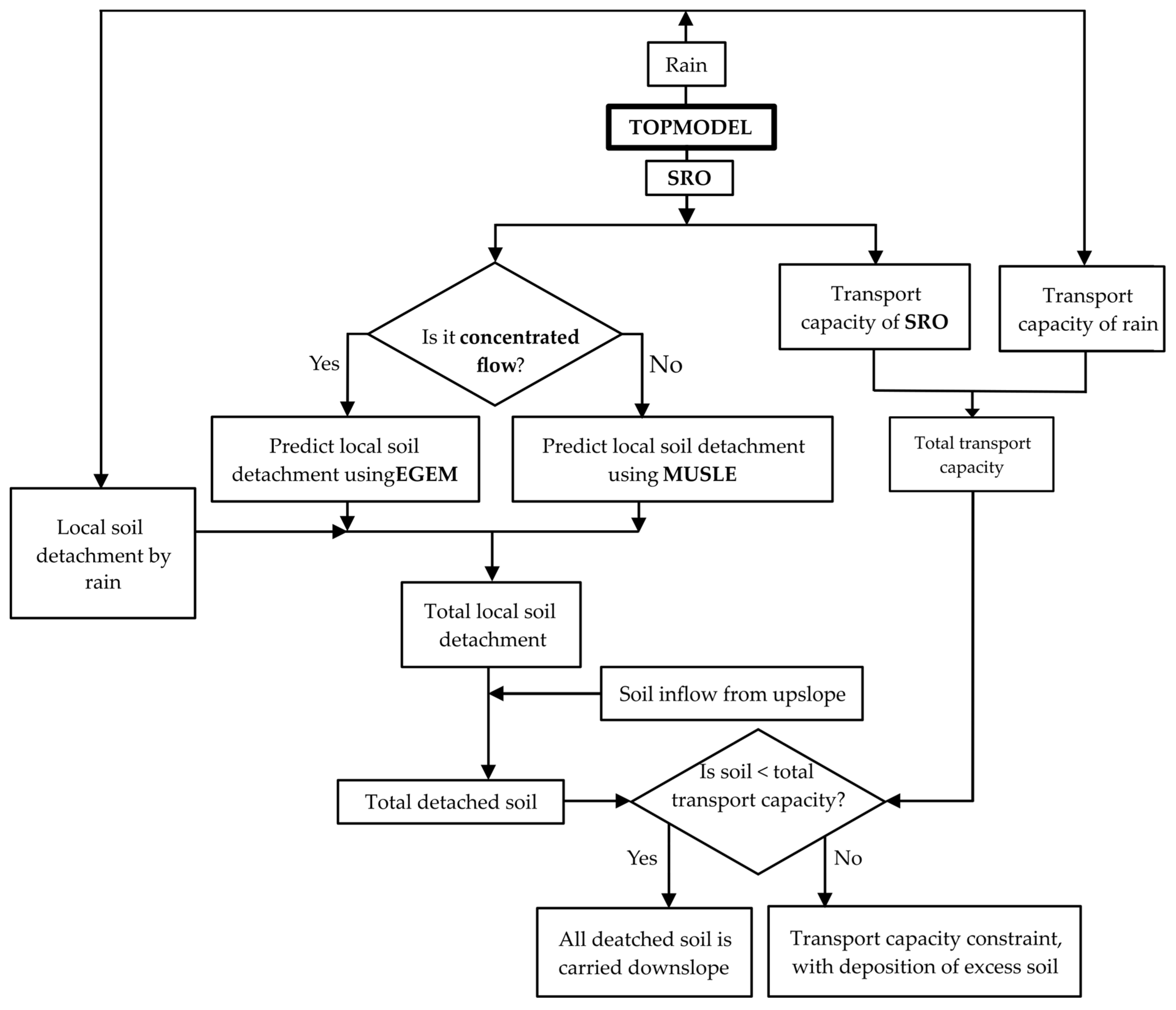
The tool for analysis, TopEros (Figure 2), integrates the TOPMODEL concept [22], the FAO56 Penman–Monteith model of reference evapotranspiration [27], and three erosion models—MUSLE [7], to predict water erosion by non-concentrated surface runoff; a model to estimate soil detachment by raindrop impact [28]; and a model to measure soil loss by concentrated flow [29]—making it an integration of 5 models.
The mathematical formulation of the model was written in Python 3.13.9 programming language. Various data types, ranging from scalars to 4-D NumPy arrays, were adopted. The primary constraint to running the model at fine spatio-temporal resolutions was computing power.

2.2.1. Hydrologic Model Component

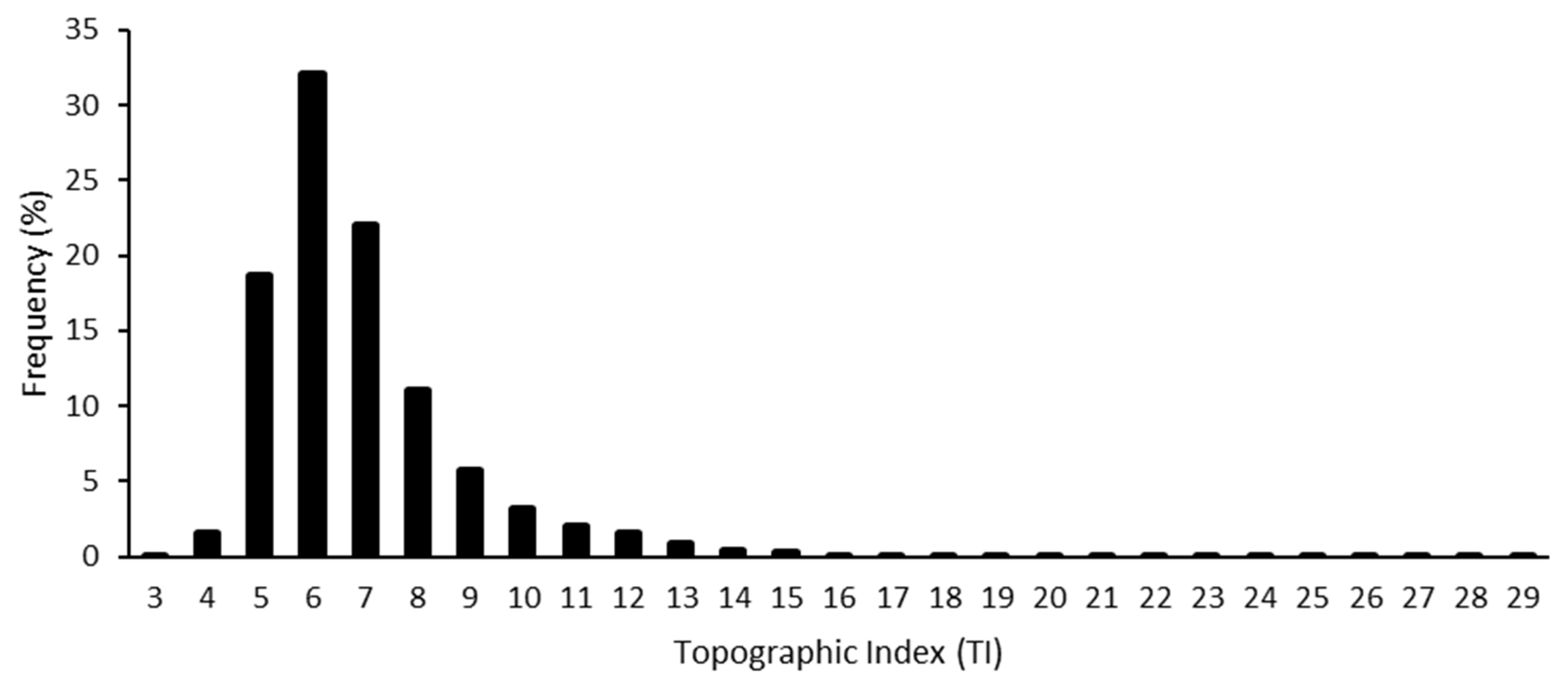
TOPMODEL is a TOPography-based hydrological model that was put forward by Beven & Kirkby [22]. It adopts the topographic index (TI), an index of hydrological similarity; i.e., cells with the same TI are assumed to have the same hydrologic response, reducing computational need. From the spatial distribution of TI (Figure A2 and Figure A3d), which is a measure of a grid cell’s propensity toward saturation, TOPMODEL is also able to track the state of saturation of the soil surface [22,30].
T I = ln a i tan β i
where ai (m) is the upstream contributing area per unit contour length [30]. Speight [31] defined it as the specific catchment area. Further, Pradhan et al. [32] defined the “unit contour length” as it pertains to a DEM as the width of a pixel. The term tan β i is the local slope, and i is the grid number under evaluation.
TOPMODEL boasts pros like being spatially distributed, flexible, and easily integrated with geographic information systems, allowing for the use of freely available gridded data. Its calibration involves the determination of parameter values like the exponential decay parameter (m), downslope transmissivity (Te), and the delay time (td). Okiria et al. [33] identified the parameter values for Atari River catchment in eastern Uganda (Figure A1). Their study also found that TOPMODEL ably reproduced the hydrological response of catchments in the Elgon region in eastern Uganda. For this reason, TOPMODEL was chosen as the hydrological module for TopEros. A detailed description of the computational procedure of this TOPMODEL can be found in [34,35,36]. Note that, during calibration, TOPMODEL was run at daily time steps with the adoption of the concept of hydrological similarity. However, when TopEros was run (TOPMODEL + erosion model), the simulation was conducted at hourly time steps, distinctly for every pixel: the concept of hydrological similarity was abandoned since we could not extend it to soil erosion. The hourly results were then summed up to daily time step at the end of every 24-h simulation.
Calibration Strategy
We calibrated TOPMODEL with the 2015 hydrological period and validated it with the data from 2016. The choice was driven by data coverage and the desire to calibrate on a period that included significant storm events while reserving an independent year for validation. The objective functions that were used to test for the model performance were the Nash–Sutcliffe Efficiency (NSE), RMSE–observations standard deviation ratio (RSR), and probability bias (PBIAS) [37,38]. Calibration used a multi-start search (randomized parameter sampling within physically plausible bounds) and ranking by NSE. The best parameter sets (Table 2) were examined for equifinality and model robustness prior to selecting a final parameter set for later hydro-erosion simulations. For monthly-averaged diagnostics, we also computed NSE on monthly mean daily stream discharges (Table 3), which provides a complementary measure of seasonal performance.

2.2.2. The Soil Erosion Component

Like in Wang et al. [14], each grid cell has an assumed channel. However, unlike their model, where each grid cell simultaneously experienced both sheet- and gully erosion, we posited that (a) all grid cells experience both detachment by raindrop and sheet erosion and (b) a grid cell whose topographic index exceeds a certain threshold also experiences gully erosion within its channels. In other words, each cell can experience sheet erosion + raindrop splash erosion, and cells with gullies in them have a duality of sheet + raindrop splash erosion and gully erosion. However, in each cell, after the erosion process, the eroded soil is carried into the assumed channel for routing to a downstream cell (note that, in non-gully cells, this hypothetical channel is just a transporter of material and does not experience gully erosion).
Next, we shall explain how TopEros calculates erosion. First, erosion and deposition processes are evaluated across the hillslope. Next, surface runoff—carrying any sediment that has not been deposited—instantaneously enters the assumed channel within each grid cell. Within this channel, additional erosion and deposition may occur, depending on if that grid cell satisfies the conditions for gully erosion. The total sediment transported by runoff through these channels is then aggregated across all grid cells to estimate the catchment-scale sediment yield. We clarify that, at this stage, TopEros does not include a routing algorithm as the relatively small size of the catchment and the absence of reservoirs make such routing unnecessary for the current application/test. Consequently, sediment that enters the channel network is assumed to be transported instantaneously to the catchment outlet for the calculation of total sediment yield.
The assumptions of the erosion module are as follows:
  • Each cell has an assumed channel, whose width is expressed by Equation (13) [21].
  • Grid cells whose topographic indices exceed a certain threshold have zones of concentrated flow and exhibit a duality of sheet + raindrop splash erosion and gully erosion, i.e., sheet erosion due to diffuse runoff in the non-channel zone of the cell, raindrop splash erosion when the soil is not saturated, and gully erosion within the channel section of the cell.
  • The hypothetical channel in each cell receives runoff and its entrained sediment for routing to a downstream cell.
The sediment yield is formulated as in Equation (2).
S Y = D s e + D f + D r S D
where SY is sediment yield, Dse is the soil detachment due to diffuse runoff, Df is the soil detachment due to concentrated flow, Dr is soil detachment by raindrop impact, and SD is sediment deposition. All units are units of mass.
Table 1. Classification of soil loss risk [39].
Erosion RiskThreshold (Mgha−1yr−1)
Very lowSoil Loss ≤ 2
Low2 ≤ Soil Loss ≤ 10
Moderate10 ≤ Soil Loss ≤ 50
High50 ≤ Soil Loss ≤ 100
Very highSoil Loss ≥ 100
Table 2. The best-performing parameter sets from the calibration of TOPMODEL in 2015. Notice the equifinality (many parameter sets with a similar skill score). The objective functions are calculated for daily averages of stream discharge. NSE_v, RSR_v, and PBIAS_v are the corresponding NSE, RSR, and PBIAS values during model validation in 2016. Note that SRZinitial was set to 0 in 2016 as the simulation commenced at the start of the rainy season.
Parameter Setm
(mm)
Te
(mm2h−1)
td
(hmm−1)
SRmax (mm)SRZinitial (mm)NSERSRPBIAS
(%)
NSE_vRSR_vPBIAS_v
130.84768790.0142.8710.0000.6160.619−4.5760.5030.7051.462
233.53273350.0123.4850.0000.6110.624−6.5190.5030.705−1.109
330.88263180.0134.2410.0000.6080.626−8.0910.5000.7071.108
419.17295750.0270.3310.0000.6010.631−5.3710.4860.7176.753
521.87963280.0203.2670.0000.6000.633−2.5130.4790.7228.378
628.40272950.0200.6810.0000.5890.6414.5540.4910.7137.673
720.71365930.0252.9280.0000.5830.64611.9300.4460.74419.357
817.97590690.0263.6050.0000.5790.6499.8930.4290.75621.818
923.43314890.0269.4260.0000.5530.66810.5090.3870.78322.468
1030.60561690.0115.5470.0000.5450.675−17.2120.4650.731−6.767
1128.79775710.0159.6780.0000.5410.67716.3380.4340.75222.765
1218.43687020.0241.7190.0000.5370.681−9.3840.4730.7267.540
1347.18768690.0087.0660.0000.5200.6935.9800.5000.707−1.375
1441.63162310.0120.1200.0000.5180.694−23.8720.4260.758−20.933
1548.83828000.0106.3400.0000.5010.7065.9160.4700.728−1.303
1620.73336110.0222.8840.0000.4520.740−16.8540.4380.7490.629
Table 3. Objective functions for monthly mean daily stream discharge during calibration and validation of TOPMODEL.
YearNSERSRPBIAS (%)
Calibration20150.8810.345−3.268
Validation20160.8790.3471.529
Detachment by Raindrop
Before becoming saturated, a cell is exposed to detachment by raindrop. Wang et al. [21] and Foster et al. [28] proposed a formulation to calculate detachment by effective raindrop energy (Equation (3)).
D r = 0.0138 K C I 2 ( 2.96 ( tan β ) 0.79 + 0.56 )
where Dr is the soil detachment rate due to raindrop (kgh−1m−2), and K (MghaMJ−1m−1) and C are USLE soil erodibility and crop management factors, respectively, while I is the effective rainfall intensity (mh−1) and β is the degree slope of the cell. We include this process for model generality as it may be significant in some catchments were saturation delays or during initial storm phases where saturation is delayed. However, we also recognize that, in rapidly saturating environments, the soil surface may quickly become protected by a water layer, limiting the effectiveness of raindrop impact.
Sheet Erosion
Detachment due to sheet erosion was estimated using MUSLE of Williams [7]. Its erosion energy factors accept a surface runoff volume and peak discharge rate. The surface runoff volume and the peak runoff rate are calculated by the hydrological model (TOPMODEL). The critical parameters for MUSLE include, among others, the physically derived slope-length factor (LSp)—a measure of the erosive force of the runoff—and the soil erodibility factor (K), a measure of the susceptibility of a soil textural class to erosion. After experimentation, van der Knijff et al. [40] developed a formulation to estimate USLE’s C factor (Equation (5)). A formulation for K was suggested by Williams [41]. Further, Moore & Burch [42] proposed a physically based formulation of the LSp factor, hinged on the “unit stream power” theory (Equation (7)).
D s e = 11 8 Q q p 0.56 K C L S p P
Dse is the sediment yield due to sheet flow (Mg); Q is the surface runoff volume (m3); qp is the peak runoff rate (m3s−1); and K, C, and P are the standard USLE factors for soil erodibility, cover management, and erosion control practice, respectively. LSp is the physically derived slope-length factor.
C = e x p α N D V I β N D V I
Parameters α and β determine the shape of the NDVI-C curve. Van der Knijff et al. [40] found that α and β of 2 and 1, respectively, yielded reasonable results in Italy. We adopted these values due to a lack of local calibration data for the C factor. We acknowledge that this introduces uncertainty as these parameters are site-specific and may not be optimal for the vegetation and agricultural conditions in our catchment.
Normalized Difference Vegetation (NDVI) is computed from Sentinel 2-imagery. NDVI values during the rainy season were selected for both 2015 and 2016.
K = 0.2 + 0.3 e x p [ 0.0256 S A N ( 1 S I L 100 ) ] S I L C L A + S I L 0.3 1 0.25 C C + e x p ( 3.72 2.95 C ) 1 0 0.7 S N 1 S N 1 + e x p 5.51 + 22 9 S N 1
SAN, SIL, CLA, and C are the percentage sand, silt, clay, and organic carbon contents of the soil and SN1 = SAN/100. The edaphic parameters were obtained from the Harmonized World Soil Data Base—Version 1.1 [43]. K is allowed to vary from 0 to 0.5.
L S p = a i 22 3 m sin β 0.0896 n
where ai is the upstream contributing area per unit width of contour, analogous to upstream contributing area per unit width of cell; β is the local degree slope; and m and n are constants. Moore & Burch [42] adopted m and n as 0.4 and 1.3, respectively. However, Moore & Wilson [44] reported that the RUSLE LS and LSp were best fitted when exponents m and n were 0.6 and 1.3, respectively. They further reported that values from 0.4 to 0.6—for m—and from 1.2 to 1.3—for n—were reasonable in representing a 3-D complex terrain, which we adopted for our analysis.
Soil Erosion by Concentrated Flow
Again, each cell experiences detachment by raindrop impact and sheet erosion. However, when the grid cell’s topographic indices exceed a given threshold, the cell will be assumed to experience concentrated flow in its channel section. The cell’s channel has assumed width dimensions. In Wang et al. [21], net flow detachment by concentrated flow occurred when (a) the hydraulic shear stress exceeded the critical shear stress of the soil and (b) the sediment load was at most equal to the sediment transport capacity of the flow. The flow detachment capacity was further described as “the gross detachment rate, assuming a uniform distribution of flow and soil erosion rates over the computational grid” [21]. Here, we modified this to assume a uniform distribution of flow and soil erosion rates over the assumed sub-grid channel reach.
Identification of the Location of Gully Erosion
Since ephemeral gully location is controlled by micro-topographies [23,45], by extension, all gully locations can be predicted through topography-derived indices. Again, TI is a measure of the tendency of a soil to become saturated. Meanwhile, the aitanβ (m) index is a measure of the erosive power of concentrated runoff. Like TI, for the aitanβ index, ai is the upstream contributing area per unit contour length and β is the local degree slope. Moore et al. [23] found that using both the TI and the aitanβ (m) index improved the prediction of gully locations in a small catchment (0.075 km2). We cautiously extend their idea to the Namatala River catchment; i.e., we adopted the use of both indices to predict gully locations.
Calculation of Gully Erosion
D f = D c h ( 1 G T c )
Df is the net detachment by concentrated flow (kgh−1m−2), Dch is the flow detachment capacity/gross detachment rate (kgh−1m−2), G (kgmin−1m−1) is sediment load—the sediment delivered to the assumed channel in the cell from its slope—and Tc is the transport capacity of the flow per unit width of catchment (kgmin−1m−1).
D c h = w K ( 1.35 τ ¯ τ c r ) 1.05
where w is the channel width (m), K is USLE’s soil erodibility factor, τ ¯   is the average shear stress for a cross-section (Pa), and τ c r is the critical shear stress (Pa). The basic form of the equation describing Dch was developed by Foster et al. [29]. A reformulation of Foster et al.’s equation was suggested in Wang et al. [21] (Equation (9)).
τ c r = 3.23 5.6 S a 24 4 o r + 0.0009 ρ d
where Sa is the fraction of sand in the soil, or is the fraction of organic matter in the soil, and ρ d is the dry bulk density of the soil (kgm−3). The formulation of τ c r is in Flanagan & Livingston [46].
τ ¯ = γ h S f
where γ (kgm−2s−2) is the specific weight of water and Sf is the friction slope. This formulation is in Wang et al. [21].
S f = n 2 u 2 R 4 3
where n is Manning’s roughness co-efficient, u (mh−1) is the depth average of channel flow velocity, and R is the hydraulic radius of the assumed channel.
w i = σ A i ε
where wi (m) is the assumed channel width at grid i of a rectangular cross-section channel, Ai is the upstream contributing area of grid i, and σ and ε are constants. In Wang et al. [21], while ε = 0.5, σ was found by entering the known channel width at the catchment outlet into Equation (13).
Transport Capacity of Flow
This is a limit on how much sediment can be carried by runoff (see illustration in Figure 2). Sediment is deposited if the sediment load exceeds the capacity of the runoff to carry it. Beasley et al. [9] proposed Equation (14) as an estimator of the transport limiting capacity under different rates of discharge. We adopt this approach because it requires only discharge per unit width—a direct output of TOPMODEL—and local slope, which is also readily available. Moreover, the formulation was recently used by Wang et al. [21] in 2010.
T c = 146 tan β . q 0 5                     f o r                       q 0.046 m 2 / min 14,600 tan β . q 2               f o r                           q > 0.046 m 2 / min
Tc is the transport capacity of the flow per unit width of catchment (kgmin−1m−1), q is the flow rate per unit width of catchment (m2min−1) [44], and tan β is the local slope.

2.3. Data

2.3.1. Meteorological Data

Daily rainfall was obtained from two rain-gauge stations (RG_1 and RG_2) and a weather station (WS) within or in the vicinity of the catchment (see Figure 1). Additionally, the WS provided four meteorological variables (relative humidity, solar radiation, wind speed, and air temperature), which were used to estimate evapotranspiration. Measurement periods used in model runs are 28 February 2015 to 31 October 2015 and 1 May 2016 to 31 December 2016. We adopted only periods with complete data coverage to avoid introducing bias from gap-filled extremes.

2.3.2. Streamflow

Daily stream discharge at the gauging station (catchment outlet) was used for calibration and validation (2015 and 2016, respectively). Discharge time series were visually inspected and subjected to standard plausibility checks (removal of obvious outliers and metadata checks against known instrumentation issues).

2.3.3. Sediment

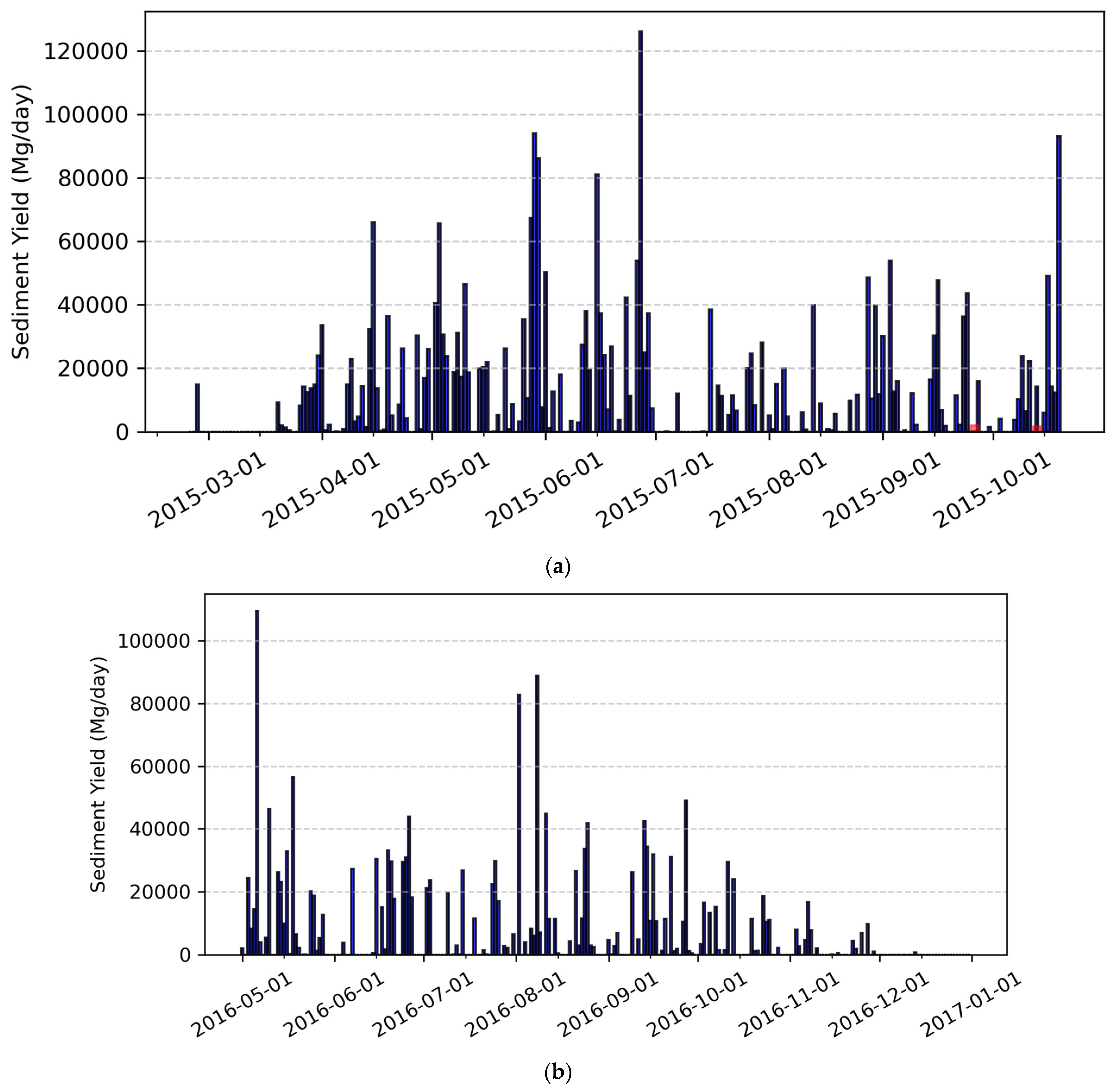
Direct catchment-scale suspended-sediment observations were not available. A bare runoff plot (0.49 × 5.00 m, slope 4.2%) located at an upland maize field within the catchment was deployed from 26 September 2015 to April 2016. Runoff and sediment from the plot were measured manually and provide a local-scale reference for erosion intensity during some storms (Figure A4). These plot measurements were used only as local ground-truth indicators and were extrapolated cautiously to explore the plausibility of catchment-scale erosion estimates (see Section 3.2.7). They were not used for any validation whatsoever. We discuss the limitations of this extrapolation in Section 3.3 and propose alternative validation strategies.

2.3.4. Geo-Spatial Data

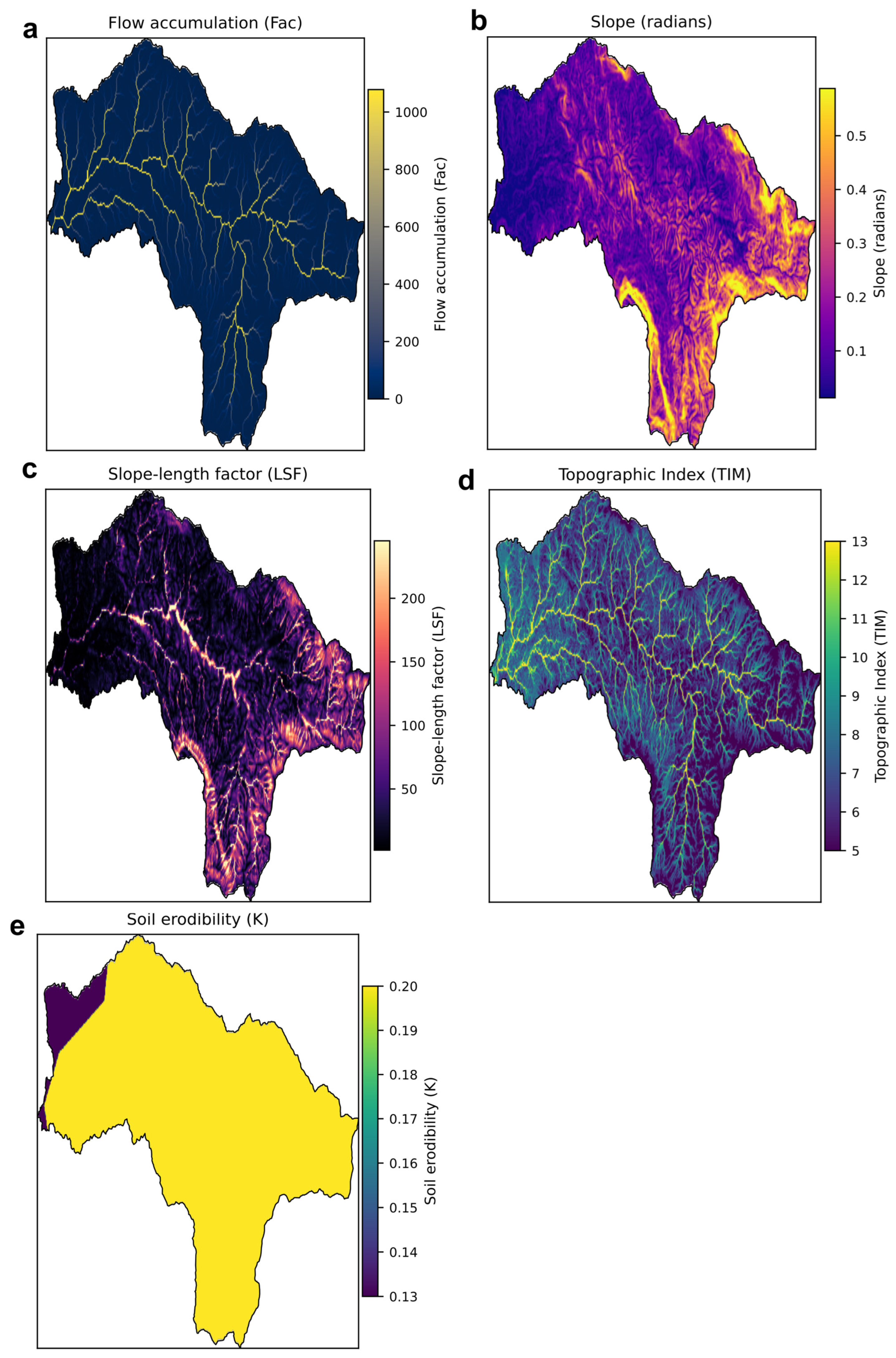
A 12.5 m resolution DEM [24], with pits filled, was used to compute topographic indices and the LSp factor, while the edaphic properties (sand, silt, clay, and organic carbon content) from the Harmonized World Soil Database v1.1 (HWSD) [43] were used to compute the soil erodibility factor K. All spatial datasets were harmonized to a 50 m grid resolution for the model simulation. The original DEM was aggregated to 50 m to reduce computational load. The edaphic properties were then resampled to the 50 m grid by assigning the parameters from the single coarse HWSD map unit to all 50 m cells within it. It is critical to note that this 50 m grid does not represent 50 m scale soil variability. As shown in Figure A3e, this approach results in near-uniform soil properties across the catchment. Thus, the spatially distributed erosion patterns predicted by TopEros are primarily driven by the topographically derived variables (slope, contributing area, and TI).
Each grid cell includes a sub-grid “assumed channel” (Equation (13)) whose width is a power-law function of contributing area following Wang et al. [21]. Runoff generated by TOPMODEL is partitioned to overland (sheet) flow and to the channel portion (where present) based on TI and aitanβ thresholds. Sediment detachment and deposition by diffuse and concentrated flow are computed separately.

2.4. Validation of the Erosion Model

Given the lack of observed catchment-scale erosion records, we were unable to validate the erosion model explicitly. We opted to adopt the following strategy to validate TopEros:
  • Comparison against running MUSLE across the entire catchment.
  • Comparison of TopEros sediment delivery ratios against those predicted by established empirical relationships (refer to Section 3.2.5).
  • Comparison of the erosion values against those from similar catchments in previous studies.
These were plausibility checks of erosion prediction by TopEros.

3. Results and Discussion

Section 3.1 will present the results of the calibration of the parameters of the hydrological model—TOPMODEL (Figure 3 and Figure 4)—while Section 3.2 will present the findings of the soil erosion models (Figure 5, Figure 6, Figure 7 and Figure 8). Finally, in Section 3.3, the limitations of TopEros and future directions will be discussed.

3.1. Calibration and Validation of TOPMODEL

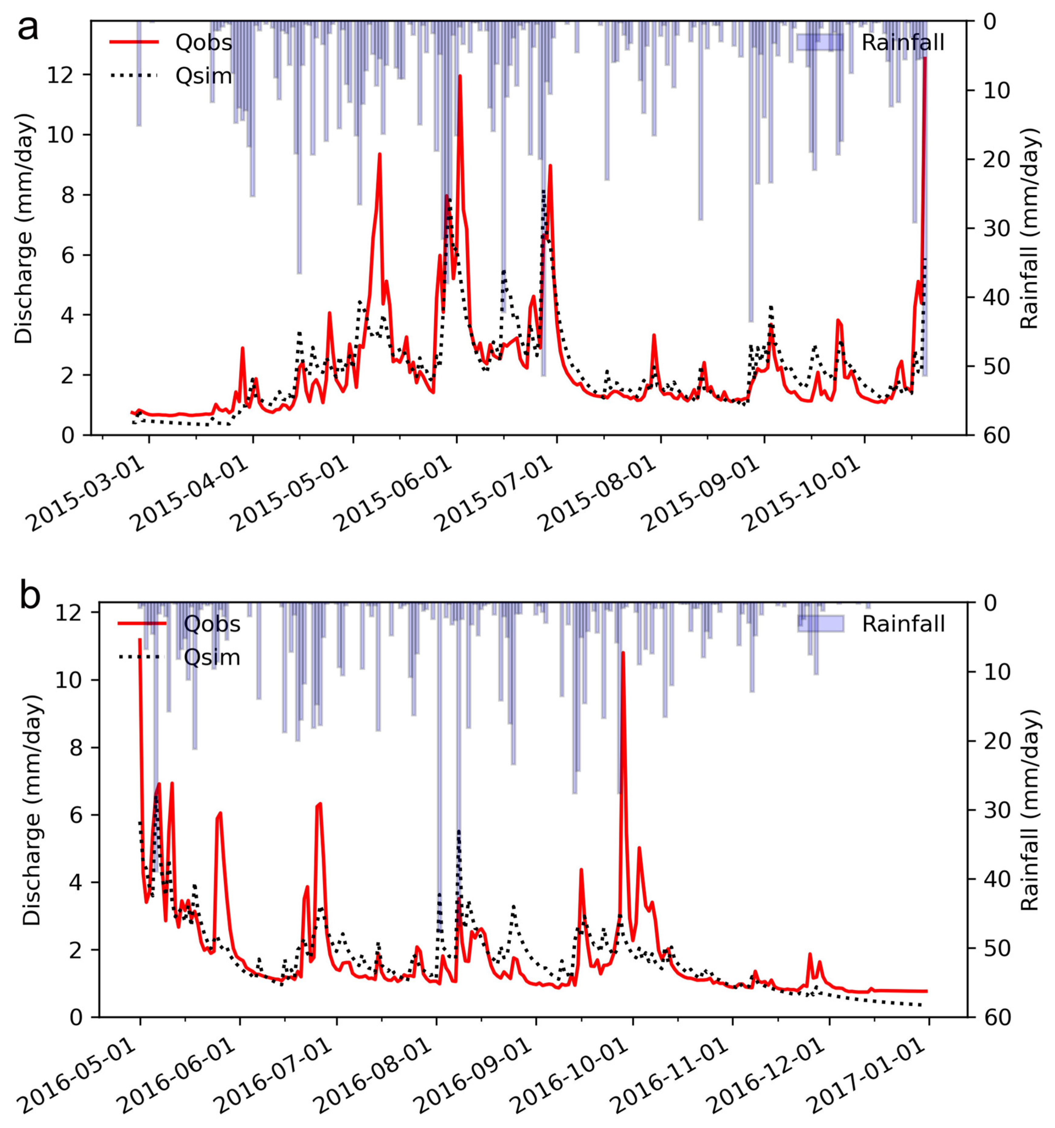
Table 2 shows the top 16 parameter sets derived from the calibration of TOPMODEL. From this table, equifinality—where many parameter sets have similar predictive performance—is evident. Through validation of the competing parameter sets against the 2016 observed discharge, the first-row parameter set of Table 2—underlined—was chosen as the most optimum, albeit marginally. NSE was 0.616 and 0.503 during calibration and validation, respectively. These values were deemed acceptable as per Moriasi et al.’s [38] guidelines. When the monthly mean daily stream discharges were considered, the NSE values increased to 0.881 and 0.879 for calibration and validation, respectively, meaning that TOPMODEL simulated seasonal variability remarkably well. For the daily averages of streamflow, RSR was 0.619 and 0.705 for the 2015 and 2016 simulations, respectively. An analysis of the monthly mean averages saw the RSR values improve to 0.345 and 0.347 for calibration and validation, respectively, again providing evidence of strong seasonal performance (Figure 4). For the daily averages of streamflow, RSR was 0.619 and 0.705 for the 2015 and 2016 simulations, respectively.
Before discussing percent bias (PBIAS), it is worth noting that different authors formulated and interpreted the metric quite differently [38,47,48,49]. In this study, we adopted the method where a positive and a negative PBIAS were synonymous with underestimation and overestimation, respectively [38,49]. For the daily stream discharge, PBIAS was −4.576% and 1.462% in calibration and validation periods, respectively: within |6.038| percentage points of each other. This was interpreted as a tendency towards the overestimation of stream discharge in 2015 and an opposite tendency in 2016; this is further visualized in Figure 3. The inconsistent observations of PBIAS during calibration and validation may seem quite baffling at first. However, given that the absolute values of PBIAS were both close to zero and within |6.038| percentage points of each other, this was deemed not to be an issue.
Figure 3 shows observed daily rainfall, observed daily discharge, and simulated daily discharge. Generally, the trends of the observed and simulated hydrographs corresponded well. Most notable was the ability of TOPMODEL to capture both small and large peaks, highlighting the robustness of the variable source area (VSA) concept of the model. A glance at the hydrographs in Figure 3 shows some instances of underprediction of stream discharge. This could be attributed to localized rainfall events that were missed by the rain gauges. Indeed, Sugawara [50] reported that tropical rainfall was highly localized, requiring multiple spatially distributed rain-gauge networks to obtain a more meaningful representation of catchment rainfall. With the same logic, the overprediction of peaks could be explained. Although the rainfall event on 15 June 2015 was captured by the rain gauge, it could have been a local event, with a minimal effect at the catchment scale, hence the higher peaks during simulation. This could be a reason for the higher simulated peak runoff compared to the observed peak after this rainfall event. When the shortcomings of GSMaP rainfall products identified by Takido et al. [51] are clarified, they—GSMaP products—could complement ground observed data, offering finer spatial resolutions [33] and a more realistic representation of catchment rainfall.
Overall, TOPMODEL robustly simulated catchment runoff, providing a strong foundation for the estimation of erosion due to runoff.

3.2. TopEros Erosion Module

With surface runoff generated by TOPMODEL as input, TopEros estimated spatially distributed soil erosion. Again, because of a lack of observed sediment time series, the correctness of this spatial distribution cannot be confirmed yet.

3.2.1. MUSLE Parameters

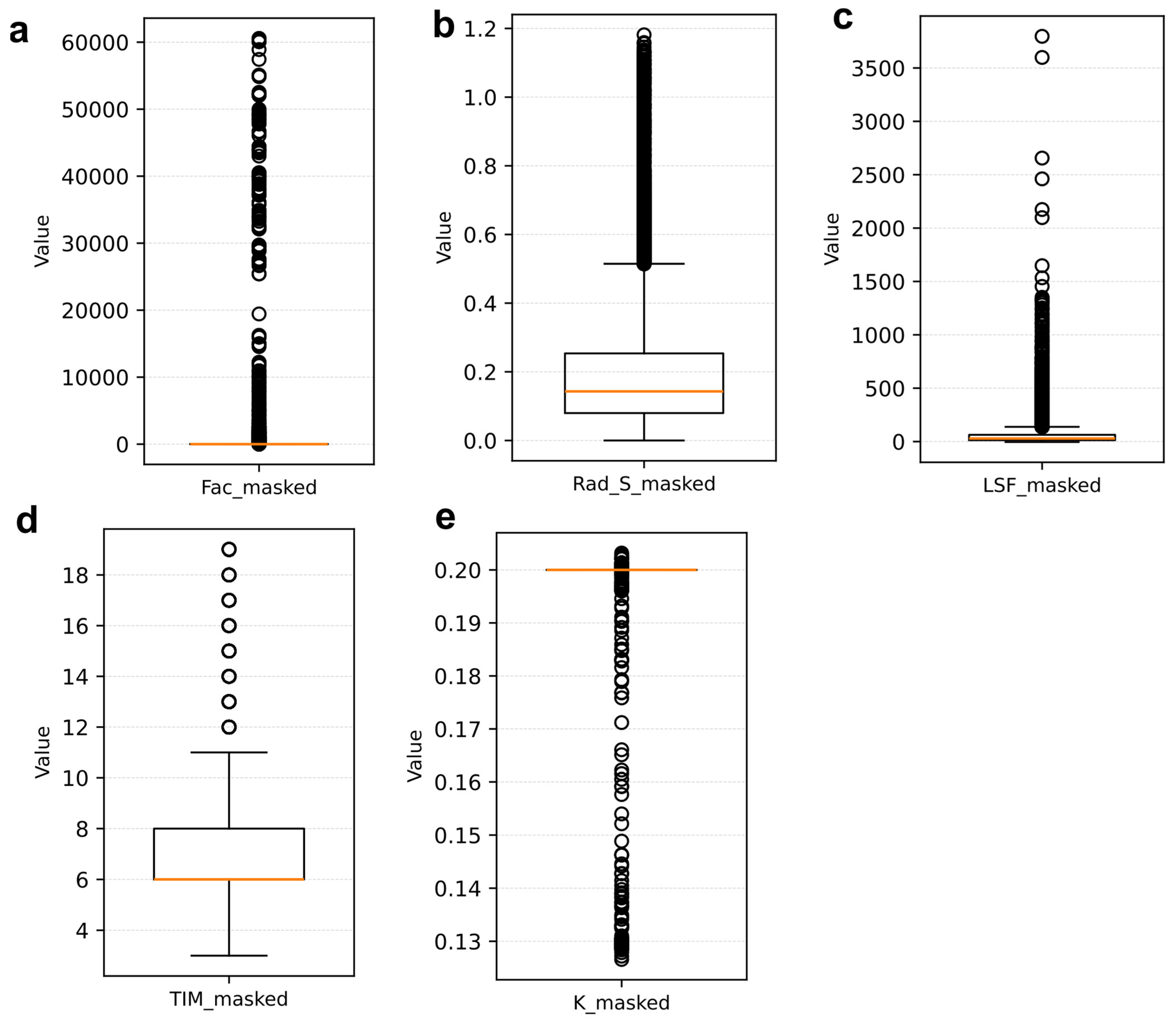
The values of the K parameter of MUSLE ranged from 0.127 to 0.204, with a median of 0.2, well within the 0 to 0.5 range defined by William’s [41] Equation (6) (see Figure A3e and Figure A5e). Meanwhile, the LSp values had a median of 28.5 and varied from 0 to 5.366 × 10⁷ (see Figure A3c and Figure A5c). Following the guidelines of Li et al. [52], for the study period, P = 1 was used because there was no evidence of human intervention for soil and water conservation measures within the catchment.

3.2.2. Threshold Values of the Topographic Indices

For the Namatala River catchment, the threshold values of TI and aitanβ at which concentrated flow was assumed to start were 15 and 35, respectively. These values predicted the channel features that could be resolved from a 12.5 × 10² m2 resolution DEM, aligning with observable stream networks. Moore et al. [23] reported threshold values of 6.8 and 18 for TI and aitanβ, respectively. TI values varying from 6.8 to 9.8 and aitanβ values stretching from 18 to 40 have also been reported [53]. Meanwhile, Daggupati et al. [54,55] reported values of 12 and 30 to 50 for TI and aitanβ, respectively. All these values were of the same order of magnitude as those used for TopEros in the Namatala River catchment. This was the first step towards an attempt at validating the erosion prediction. With the identification of topographic-index thresholds, it became possible to classify cells with and without concentrated flow. The caveat is that the threshold values of topographic indices for locating ephemeral gullies could be site-specific.

3.2.3. Sediment Yield at the Catchment Outlet

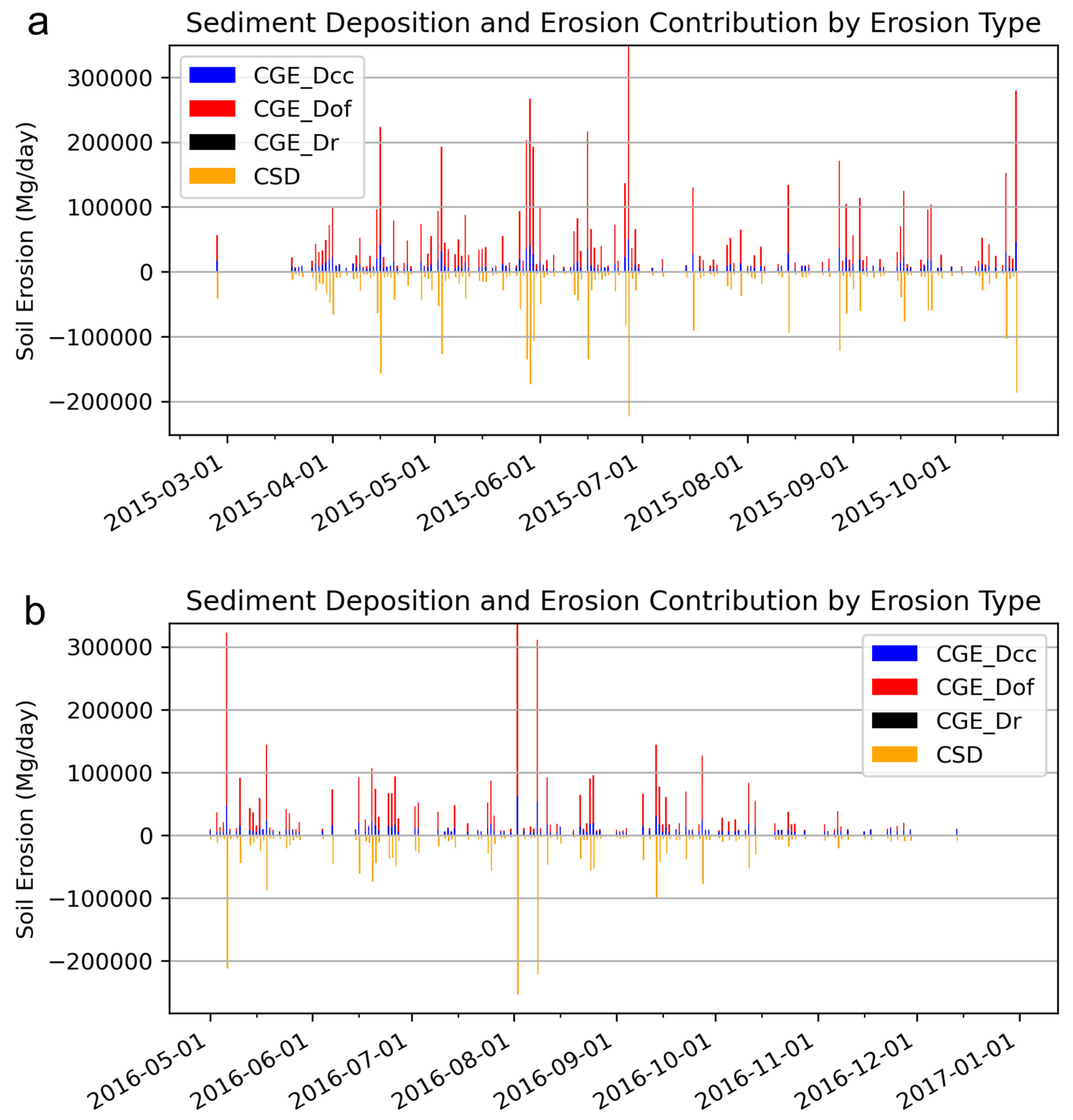
Although the in situ observations of rainfall for 2015 (28 February to 31 October) and 2016 (1 May to 31 December) were incomplete, they captured most of the bimodal rainfall in the Namatala River catchment—April to May and August to October [56]. Therefore, annualized units—Mgyr−1—provide reasonable approximations of soil erosion. Table 4 and Figure 5 summarize the sediment yields and deposition and erosion components as simulated by TopEros.
To benchmark the results of TopEros, we also applied MUSLE to the entirety of the catchment. In 2015, TopEros estimated a catchment sediment yield (CSY) of 2.387 × 10⁶ Mgyr−1 compared to 2.915 × 10⁶ Mgyr−1 from MUSLE. In 2016, the corresponding values were 1.443 × 10⁶ and 1.774 × 10⁶ Mgyr−1, respectively. The tendency of USLE-type models to overpredict sediment yield under high-intensity rainfall has been documented [57]. Desmet & Govers [20] and Wischmeir & Smith [5] attributed it to non-consideration of the sediment deposition process by USLE-type models. However, here, even with the incorporation of sediment deposition, MUSLE still overpredicted sediment yield, exceeding TopEros by approximately 20% in both years. This could be due to overestimation of the LSp factor in the channels (see Figure A3c).

3.2.4. Partitioning of the Erosion Process

TopEros enables decomposition of gross erosion into process-specific components. In 2015, sheet (overland) erosion dominated, contributing 68% (4.438 × 10⁶ Mgyr−1), and, in 2016, it contributed 60% (2.714 × 10⁶ Mgyr−1). Given that approximately 90% of the catchment area is prone to sheet erosion (according to TopEros), these proportions are plausible. Concentrated flow (gully) detachment accounted for the remaining 32% (2.090 × 10⁶ Mgyr−1) in 2015 and 40% (1.839 × 10⁶ Mgyr−1) in 2016, falling within the reported gully-erosion contribution range of 10–94% [4,58]. Raindrop detachment was negligible, likely due to rapid surface saturation reducing raindrop impact energy. It is also possible that the climatic and cover management factors in Equation (3) did not consider the effect of throughfall from raindrops that consolidate into larger drops in forested areas with minimal understory or litter, thereby underestimating erosion by raindrop impact. In their review, Labrière et al. [2] reported that raindrop amalgamation over large leaves carries more kinetic energy on impact and therefore has greater potential for soil detachment in forested areas without undergrowth.
Yet, compared to MUSLE, TopEros partitions erosion by type. Although the accuracy cannot be confirmed in the absence of observed data, this shows promise in understanding the advancement of erosion in a catchment.

3.2.5. Specific Erosion and Sediment Delivery Ratios

To normalize the catchment area and focus on erosion severity, specific soil loss metrics were calculated (Table 5).
Again, we start with benchmarking TopEros against MUSLE. For specific sediment yield (CSY), TopEros yielded 155 and 94 Mgha−1yr−1 versus 190 and 115 Mgha−1yr−1 from MUSLE. The sediment delivery ratio (SDR) further illuminates transport efficiency: TopEros’ SDRs were 0.366 (in 2015) and 0.317 (in 2016), whereas MUSLE predicted 0.441 and 0.456 in 2015 and 2016, respectively. The empirical relationship of Vanoni [59] for catchments of this size suggests an SDR of 0.252 ([59,60,61]). TopEros’ closer agreement with Vanoni’s benchmark could suggest improved handling of within-catchment erosion and deposition processes. Again, this must be confirmed with observed data.
Secondly, we compared the simulations of TopEros for the Namatala River catchment to those from studies on catchments with similar topography and climate. In various Rwandan catchments, Karamage [62] reported erosion rates ranging from 94 to 678 Mgha−1yr−1 using RUSLE. It is worth noting that these values might be higher than the actual sediment yield because there was no evidence that they accounted for sediment deposition. Similarly, by applying RUSLE to the Manafwa River catchment, a headwater catchment of Mt. Elgon in Uganda, Jiang et al. [39] reported sediment yields ranging from 67 to 103 Mgha−1yr−1. From their review of observed sediment yields in humid tropical climates globally, Labrière [2] reported annual erosion rates of 1 to 16 Mgha−1yr−1 in humid West African catchments. They also reported values of 0.1, 2, and 5 Mgha−1yr−1 in old-growth trees and tree crops with and without contact cover, respectively. Meanwhile, for humid West African catchments, Morgan [63] reported annual erosion rates of 0.03 to 1, 0.1 to 90, and 10 to 750 Mgha−1yr−1 in natural, cultivated, and bare-soil land cover, respectively, and 1 to 5, 8 to 42, and 5 to 70 Mgha−1yr−1, respectively, in tropical climates in Ethiopia. That TopEros does not deviate much from these values provides an early indication that its simulations are at least comparable to other models. It would require observed data to confirm how TopEros fares against these other models.

3.2.6. Spatial Patterns and Risk Classification

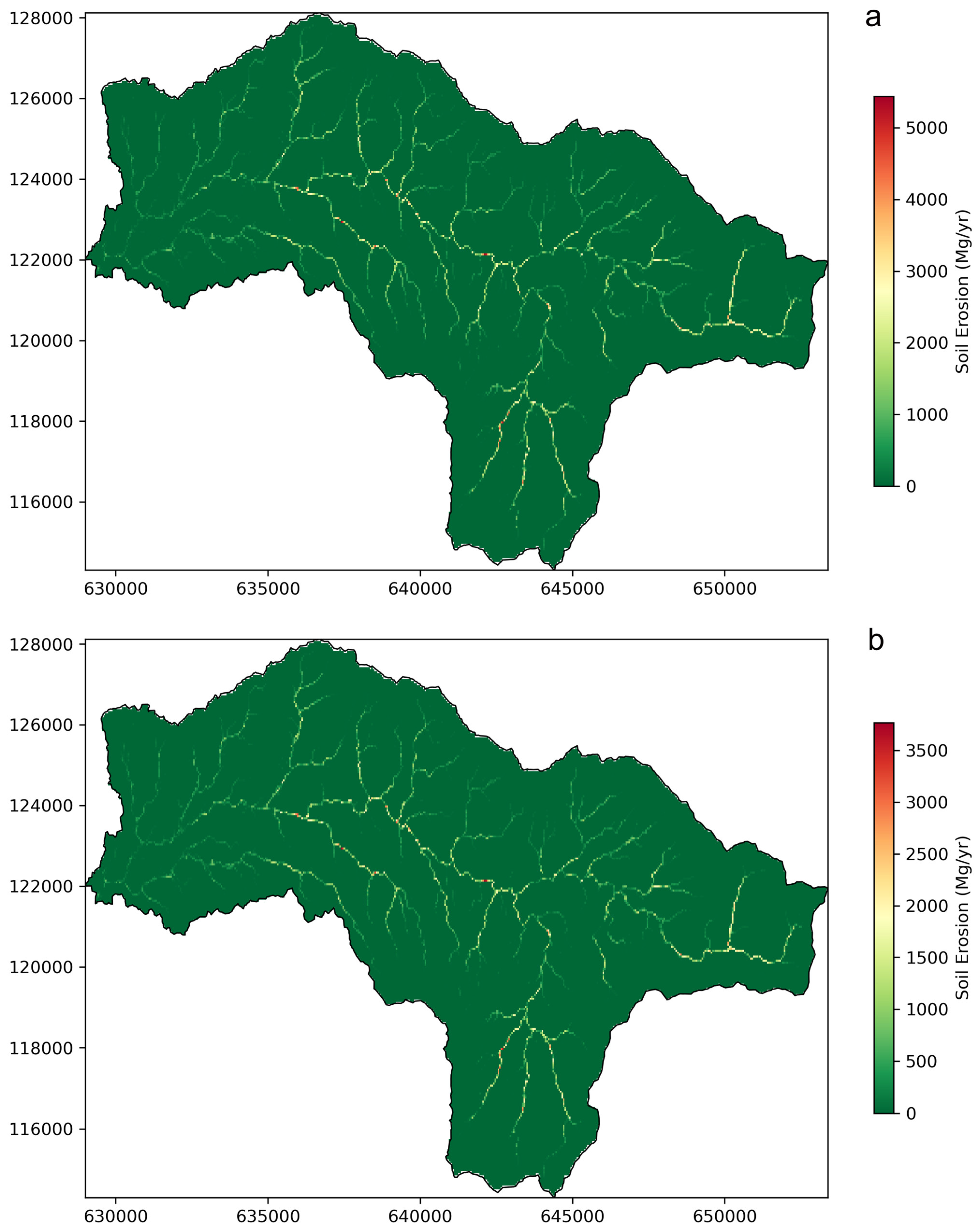
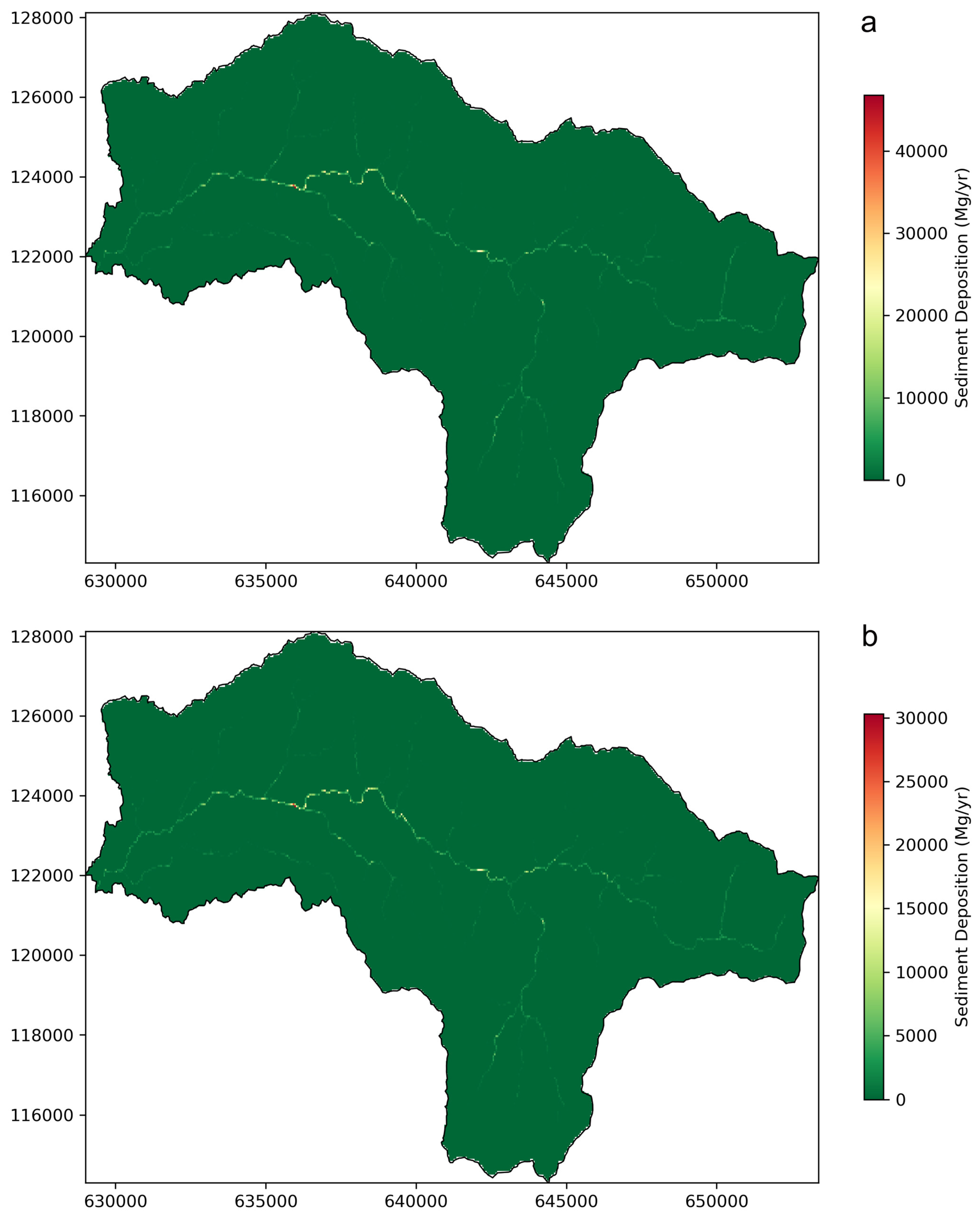
Figure 6 and Figure 7 illustrate the spatial distribution of annual erosion and deposition. High-erosion hotspots coincided with steep slopes and sparse vegetative cover, while depositional zones clustered in valley bottoms. This spatially explicit output, when verified, could be invaluable for prioritizing conservation measures.
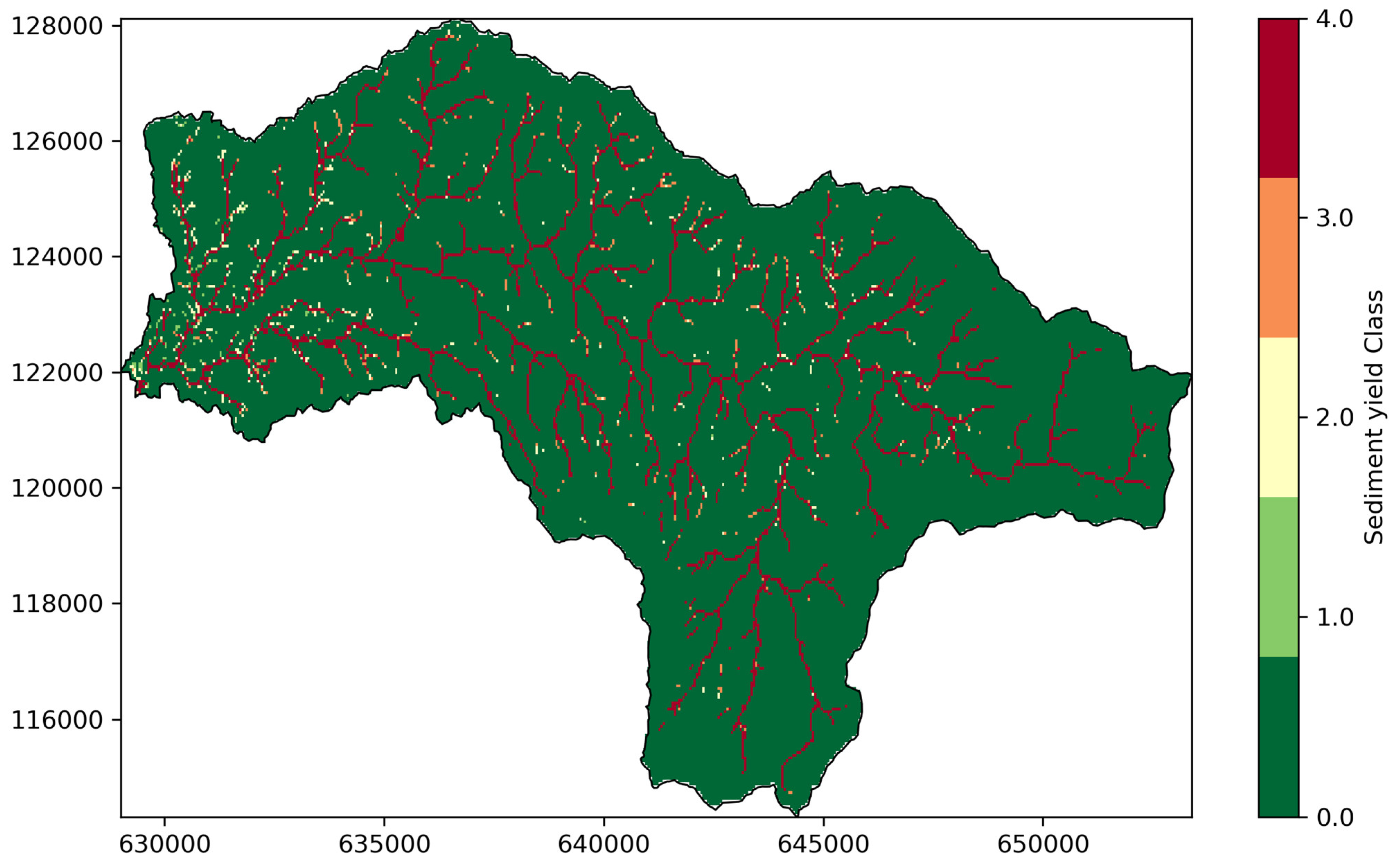
Integrating these results into erosion-risk classes [39] yields a catchment-wide classification of “very high” risk in 2015 and “high” in 2016 (Figure 8). However, the gully zones exhibited “very high” risk irrespective of year, whereas the non-channel areas largely fell into the “low” or “very low” classes. Indeed, gullies enhance sediment connectivity, allowing more sediment to reach the catchment outlet even when they cover a limited portion of the catchment [64]. This dichotomy highlights the necessity of focused interventions in ephemeral gully networks, supplementing broader sheet-erosion controls.

3.2.7. Model Validation and Implications

In lieu of direct sediment data, we judged model realism by consistency with known catchment behavior. Firstly, the locations of large predicted gullies align with field-observed channel networks. We also successfully calibrated and validated the runoff model, increasing confidence in the runoff input into the erosion module. Additionally, we found that the SDR predicted by TopEros closely approximated the values predicted by the empirical relationship proposed by Vanoni [59]. Finally, we compared the results from TopEros to those from applying MUSLE in the entire catchment. We went further and compared the predictions by TopEros to simulations by RUSLE in catchments in Rwanda and Uganda. A comparison was also conducted with in situ data in humid tropical climates. Taken together, these increase confidence in the credibility of TopEros’ predictions despite lacking in situ measurements. Future work could target implementing the model in data-rich areas to enable a complete distinct validation of the model.
Direct catchment-scale suspended-sediment observations were not available for the Namatala catchment. In place of a continuous sediment record, we used (i) the local bare-soil runoff plot (Figure A4) as a plot-scale reference, although this is remarkably insufficient and represents a measure of a localized insignificant portion of the catchment, and (ii) comparisons against independent benchmarks (MUSLE applied to the whole catchment and the empirical Vanoni relationship for SDR) and literature values from analogous catchments. Together, these comparisons provide three complementary lines of evidence.
These indirect validations increase confidence in TopEros’ physical realism but do not replace the need for continuous suspended-sediment observations. We therefore present our results as plausible process-based estimates that motivate (1) targeted sediment monitoring in the catchment and (2) validation of TopEros by application in data-rich catchments.

3.3. Limitations and Future Directions

While TopEros shows promise, its limitations point to future work. The principal limitation is the lack of continuous catchment-scale suspended-sediment measurements in the study area. Many parameters for the erosion component of TopEros were adopted from previous studies, and it is important to confirm their correctness. Moreover, ephemeral gullies are not yet explicitly modeled: their detection could be enhanced by incorporating high-resolution optical imagery and or high-resolution DEM analysis. Similarly, the model’s robustness should be tested by extending it to other catchments of the Mt. Elgon region and beyond (especially those with sediment measurements). The model should also consider slope collapse, among other debris flows within a catchment. Additionally, the use of coarse global soil data was a key limitation, and future work at small- to medium-catchment scales could benefit from local high-resolution soil-mapping datasets. Finally, incorporating a flow-routing algorithm into TopEros could first improve model performance for larger catchments and second be a prerequisite for future extension of the model to studies of global soil erosion.
Addressing these limitations would permit rigorous quantitative validation of TopEros and strengthen its utility as a decision-support tool in data-scarce tropical catchments.

4. Conclusions

TopEros is meant to address the inability of traditional USLE-type models to simulate gully erosion or gully erosion models to predict sheet erosion. We adopt the strategy of dividing the catchment into sheet-erosion and gully-erosion zones through the adoption of thresholds of two topographic indices—TI and aitanβ—to each grid cell. By deriving cell-specific topographic-index thresholds, TopEros dynamically predicted zones of ephemeral gully formation and applied the most appropriate erosion law in each domain.
When applied to the Namatala River catchment in eastern Uganda, TopEros shows promise in reproducing both annual and sub-grid variability in sediment yield. Compared to the empirically derived MUSLE, TopEros achieved sediment delivery ratios—SDR = 0.366 and 0.317 in 2015 and 2016, respectively—much closer to the Vanoni benchmark of 0.252 and partitioned gross erosion into process proportions—sheet vs. gully vs. raindrop detachment—although realism is yet to be confirmed. We cautiously think this might point to an enhanced representation of physical erosion and in-catchment deposition processes by TopEros.
TopEros thus shows promise in bridging the gap between plot-scale empirical models and catchment-scale process models through the integration of distinct detachment mechanisms within a single spatially distributed framework. This advancement not only points to potential improvements in the conceptualization of hydro-erosion dynamics at landscape scales but also potentially enables the generation of erosion-risk maps that pinpoint critical hotspots for conservation interventions.
For future work, we recommend the following:
  • Cross-catchment validation with observed sediment-yield records to quantify TopEros’ predictive gains over conventional models.
  • Enhanced gully detection, leveraging high-resolution optical and DEM data, topographic-wetness indices, and targeted field surveys to improve the delineation of ephemeral features.
  • Integration of flow-routing modules to extend the model’s applicability to larger basins and facilitate eventual upscaling to regional or global soil erosion assessments.
By addressing these limitations, TopEros has the potential to become a robust tool for both scientific research and practical catchment management, ultimately supporting more strategic data-driven soil and water conservation planning.

Author Contributions

E.O. and N.K. developed the concept and designed the experiment; E.O. wrote the TopEros model code; Y.K. and E.O. collected and processed the input data; E.O. conducted the experiment; E.O. wrote the manuscript with contributions from S.-i.N., N.K. and Y.K. All authors have read and agreed to the published version of the manuscript.

Funding

This work was supported by JSPS KAKENHI Grant Number 21H05002.

Data Availability Statement

TopEros code and input data can be downloaded from https://zenodo.org/records/15575730 (accessed on 13 November 2025).

Conflicts of Interest

Author Yukimitsu Kobayashi is employed by NTC-International Co., Ltd. The remaining authors declare that the research was conducted in the absence of any commercial or financial relationships that could be construed as a potential conflict of interest.

Appendix A

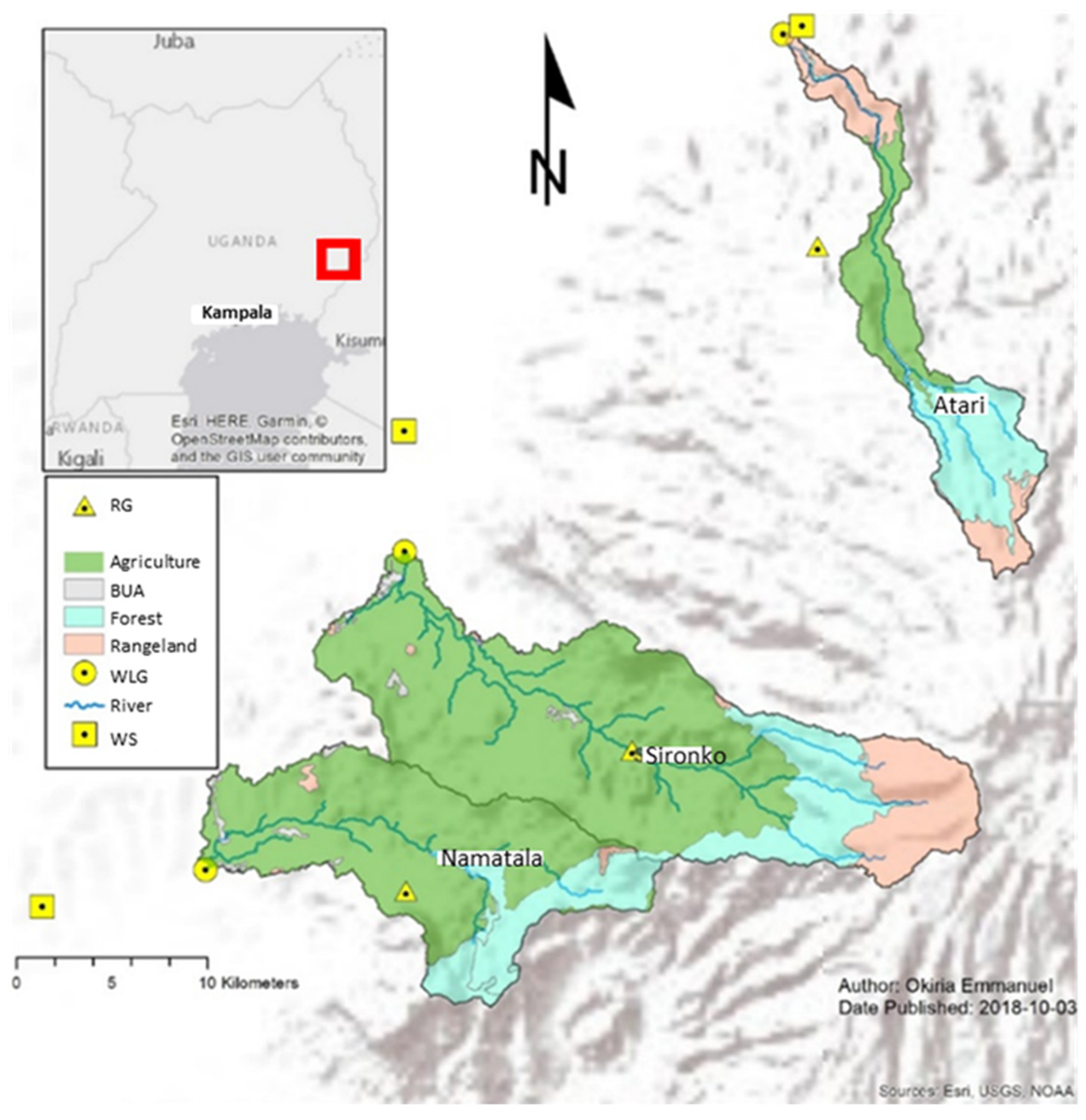
Figure A1. Instrumentation and land cover of the Namatala, Atari, and Sironko River catchments. Note that RG is rain gauge, WLG is water-level gauge, WS is weather station and BUA is built up area. The red box indicates the location of the three catchments on the map of Uganda.
Hydrology 12 00309 g0a1
Figure A2. Topographic index distribution of Namatala catchment at 50 m grid resolution.
Hydrology 12 00309 g0a2
Figure A3. Spatial distribution of select topographic and edaphic values. Panel (a) shows flow accumulation, panel (b) shows slope, panel (c) shows slope-length factor, panel (d) shows topographic index and panel (e) shows soil erodibility. Where applicable, units are described in the main text. For flow accumulation, the values are counts of cells contributing flow to the cell of interest.
Hydrology 12 00309 g0a3
Figure A4. Daily sediment yield in Namatala River catchment. Panels (a,b) are as predicted in 2015 and 2016, respectively. The red markers in panel (a) are the sediment yield observed from a bare runoff plot within the catchment: Assuming a homogeneous catchment, this sediment yield was extrapolated to the entire Namatala River catchment. The runoff plot was installed on a typical upland maize cultivation field at the Mbale District production offices. Its dimensions were 0.49 × 5 m, with the length oriented towards the outlet at a gradient of 4.2%. The surface was kept bare during the observation period from 26 September 2015 to April 2016. Runoff from the plot was collected by a bucket placed in a hole dug at the outlet of the runoff plot. Rainfall at the plot site was measured manually.
Hydrology 12 00309 g0a4
Figure A5. Boxplots of select topographic and edaphic properties. Panel (a) shows flow accumulation, panel (b) shows slope, panel (c) shows slope-length factor, panel (d) shows topographic index and panel (e) shows soil erodibility. The orange horizontal bars indicate the median, while whiskers indicate the 1.5 × IQR bounds. Where applicable, units are described in the main text. The boxplot properties correspond to those shown in Figure A3. For flow accumulation, the values are counts of cells contributing flow to the cell of interest.
Hydrology 12 00309 g0a5

References

  1. Gruver, J.B. Prediction, Prevention and Remediation of Soil Degradation by Water Erosion. Nat. Educ. Knowl. 2013, 4, 2. [Google Scholar]
  2. Labrière, N.; Locatelli, B.; Laumonier, Y.; Freycon, V.; Bernoux, M. Soil Erosion in the Humid Tropics: A Systematic Quantitative Review. Agric. Ecosyst. Environ. 2015, 203, 127–139. [Google Scholar] [CrossRef]
  3. Nkonge, L.K.; Gathenya, J.M.; Kiptala, J.K.; Cheruiyot, C.K.; Petroselli, A. An Ensemble of Weight of Evidence and Logistic Regression for Gully Erosion Susceptibility Mapping in the Kakia-Esamburmbur Catchment, Kenya. Water 2023, 15, 1292. [Google Scholar] [CrossRef]
  4. Poesen, J.; Nachtergaele, J.; Verstraeten, G.; Valentin, C. Gully Erosion and Environmental Change: Importance and Research Needs. Catena 2003, 50, 91–133. [Google Scholar] [CrossRef]
  5. Wischmeier, W.H.; Smith, D.D. Predicting Rainfall Erosion Losses: A Guide to Conservation Planning; No. 537; Department of Agriculture, Science and Education Administration: Washington, DC, USA, 1978.
  6. Renard, K.G.; Foster, G.R.; Yoder, G.C.; McCool, D.K. RUSLE Revisited: Status, Questions, Answers and the Future. J. Soil Water Conserv. 1994, 49, 213–220. [Google Scholar] [CrossRef]
  7. Williams, J.R. Testing the Modified Universal Soil Loss Equation. In Proceedings of the Workshop on Estimating Erosion and Sediment Yield on Rangelands, Tucson, AZ, USA, 7–9 March 1981; Burroughs, E.R., Jr., Chugg, J.C., Dissmeyer, G.E., Farrell, D.A., Foster, G.R., Gebhardt, K.A., Hart, G.E., Johnson, C.W., Laflen, J.M., Lane, L.J., et al., Eds.; U.S. Department of Agriculture, Agricultural Research Service, Agricultural Reviews and Manuals ARM-W: Tucson, AZ, USA, 1982; pp. 157–165. [Google Scholar]
  8. Neitsch, S.L.; Arnold, J.G.; Kiniry, J.R.; Williams, J.R. Soil & Water Assessment Tool Theoretical Documentation Version 2009; Texas Water Resources Institute: College Station, TX, USA, 2011; pp. 1–647. [CrossRef]
  9. Beasley, D.B.; Huggins, L.F.; Monke, E.J. ANSWERS: A Model for Watershed Planning. Trans. Am. Soc. Agric. Eng. 1980, 23, 938–944. [Google Scholar] [CrossRef]
  10. Wicks, J.M.; Bathurst, J.C. SHESED: A Physically Based, Distributed Erosion and Sediment Yield Component for the SHE Hydrological Modelling System. J. Hydrol. 1996, 175, 213–238. [Google Scholar] [CrossRef]
  11. Ewen, J.; Parkin, G.; O’Connell, P.E. SHETRAN: Distributed River Basin Flow and Transport Modeling System. J. Hydrol. Eng. 2000, 5, 250–258. [Google Scholar] [CrossRef]
  12. Cerdà, A.; Brazier, R.; Nearing, M.; de Vente, J. Scales and Erosion. Catena 2013, 102, 1–2. [Google Scholar] [CrossRef]
  13. Foster, G.R. Modeling the Erosion Process. In Hydrologic Modeling of Small Watersheds; Haan, C.T., Johnson, H.P., Brakensiek, D.L., Eds.; ASAE: Washington, DC, USA, 1982; pp. 295–380. [Google Scholar]
  14. Wang, G.; Jiang, H.; Xu, Z.; Wang, L.; Yue, W. Evaluating the Effect of Land Use Changes on Soil Erosion and Sediment Yield Using a Grid-Based Distributed Modelling Approach. Hydrol. Process 2012, 26, 3579–3592. [Google Scholar] [CrossRef]
  15. Sadeghi, S.H.R.; Mizuyama, T. Applicability of the Modified Universal Soil Loss Equation for Prediction of Sediment Yield in Khanmirza Watershed, Iran. Hydrol. Sci. J. 2007, 52, 1068–1075. [Google Scholar] [CrossRef]
  16. Sadeghi, S.H.R.; Gholami, L.; Khaledi Darvishan, A.; Saeidi, P. A Review of the Application of the MUSLE Worldwide. Hydrol. Sci. J. 2014, 59, 365–375. [Google Scholar] [CrossRef]
  17. Gwapedza, D.; Hughes, D.A.; Slaughter, A.R. Spatial Scale Dependency Issues in the Application of the Modified Universal Soil Loss Equation (MUSLE). Hydrol. Sci. J. 2018, 63, 1890–1900. [Google Scholar] [CrossRef]
  18. Thakuriah, G. GIS-Based Revised Universal Soil Loss Equation for Estimating Annual Soil Erosion: A Case of Lower Kulsi Basin, India. SN Appl. Sci. 2023, 5, 81. [Google Scholar] [CrossRef]
  19. Moore, I.D.; Wilson, J.P.; Ciesiolka, C.A. Soil Erosion Prediction and GIS: Linking Theory and Practice. In Proceedings of the International Conference on Application of Geographic Information Systems to Soil Erosion Management, Taiyuan, China, 2–11 June 1992; pp. 31–48. [Google Scholar]
  20. Desmet, P.J.J.; Govers, G. A GIS Procedure for Automatically Calculating the USLE LS Factor on Topographically Complex Landscape Units. J. Soil Water Conserv. 1996, 51, 427–433. [Google Scholar] [CrossRef]
  21. Wang, G.; Hapuarachchi, H.A.P.; Takeuchi, K.; Ishidaira, H. Grid-Based Distribution Model for Simulating Runoff and Soil Erosion from a Large-Scale River Basin. Hydrol. Process 2010, 24, 641–653. [Google Scholar] [CrossRef]
  22. Beven, K.J.; Kirkby, M.J. A Physically Based, Variable Contributing Area Model of Basin Hydrology. Hydrol. Sci. J. 1979, 24, 43–69. [Google Scholar] [CrossRef]
  23. Moore, I.D.; Burch, G.J.; Mackenzie, D.H. Topographic Effects on the Distribution of Surface Soil Water and the Location of Ephemeral Gullies. Trans. ASAE 1988, 31, 1098–1107. [Google Scholar] [CrossRef]
  24. Japan Aerospace Exploration Agency (JAXA); Ministry of Economy, Trade and Industry (METI). ALOS PALSAR Radiometric Terrain Corrected (RTC)—High Resolution; Alaska Satellite Facility Distributed Active Archive Center (ASF DAAC). 2014. Available online: https://www.earthdata.nasa.gov/data/catalog/asf-alos-psr-rtc-high-1 (accessed on 18 October 2023).
  25. Ferguson, C.R.; Pan, M.; Oki, T. The Effect of Global Warming on Future Water Availability: CMIP5 Synthesis. Water Resour. Res. 2018, 54, 7791–7819. [Google Scholar] [CrossRef]
  26. Singh, V.P. Watershed Modeling. In Computer Models of Watershed Hydrology; Singh, V.P., Ed.; Water Resources Publications: Littleton, CO, USA, 1995; pp. 1–20. ISBN 0-918334-91-8. [Google Scholar]
  27. Allen, R.G.; Luis, S.P.; RAES, D.; Smith, M. FAO Irrigation and Drainage Paper No. 56. Crop Evapotranspiration (Guidelines for Computing Crop Water Requirements). Irrig. Drain. 1998, 300, 300. [Google Scholar] [CrossRef]
  28. Foster, G.R.; Lombardi, F.; Moldenhauer, W.C. Evaluation of Rainfall-Runoff Erosivity Factors for Individual Storms. Trans. ASAE 1982, 25, 124–129. [Google Scholar] [CrossRef]
  29. Foster, G.R.; Meyer, L.D.; Onstad, C.A. Erosion Equation Derived From Basic Erosion Principles. Trans. ASAE 1977, 20, 678–682. [Google Scholar] [CrossRef]
  30. Quinn, P.F.; Beven, K.J.; Lamb, R. The Ln(a/Tanβ) Index: How to Calculate It and How to Use It Within the TOPMODEL Framework. Hydrol. Process. 1995, 9, 161–182. [Google Scholar] [CrossRef]
  31. Speight, J.G. The Role of Topography in Controlling Throughflow Generation: A Discussion. Earth Surf. Process. 1980, 5, 187–191. [Google Scholar] [CrossRef]
  32. Pradhan, N.R.; Ogden, F.L.; Tachikawa, Y.; Takara, K. Scaling of Slope, Upslope Area, and Soil Water Deficit: Implications for Transferability and Regionalization in Topographic Index Modeling. Water Resour. Res. 2008, 44, 1–12. [Google Scholar] [CrossRef]
  33. Okiria, E.; Okazawa, H.; Noda, K.; Kobayashi, Y.; Suzuki, S.; Yamazaki, Y. A Comparative Evaluation of Lumped and Semi-Distributed Conceptual Hydrological Models: Does Model Complexity Enhance Hydrograph Prediction? Hydrology 2022, 9, 89. [Google Scholar] [CrossRef]
  34. Beven, K.J. Rainfall-Runoff Modelling: The Primer, 2nd ed.; Wiley-Blackwell: West Sussex, UK, 2012; ISBN 978-0-470-71459-1. [Google Scholar]
  35. Hornberger, G.M.; Wiberg, P.L.; Raffensperger, J.P.; D’Odorico, P. Elements of Physical Hydrology, 2nd ed.; Johns Hopkins University Press: Baltimore, MD, USA, 2014; ISBN 978-1-4214-1373-0. [Google Scholar]
  36. Mukae, K.; Miwa, K.; Okazawa, H. Ecosystem Service Assessment in Agricultural Watershed by Using TOPMODEL. AGROFO Int. J. 2017, 2, 27–36. [Google Scholar] [CrossRef]
  37. Foglia, L.; Hill, M.C.; Mehl, S.W.; Burlando, P. Sensitivity Analysis, Calibration, and Testing of a Distributed Hydrological Model Using Error-Based Weighting and One Objective Function. Water Resour. Res. 2009, 45, W06427. [Google Scholar] [CrossRef]
  38. Moriasi, D.N.; Arnold, J.G.; Liew, M.W.V.; Bingner, R.L.; Harmel, R.D.; Veith, T.L. Model Evaluation Guidelines for Systematic Quantification of Accuracy in Watershed Simulations. Trans. Am. Soc. Agric. Eng. 2007, 50, 885–900. [Google Scholar]
  39. Jiang, B.; Bamutaze, Y.; Pilesjö, P. Climate Change and Land Degradation in Africa: A Case Study in the Mount Elgon Region, Uganda. Geo-Spat. Inf. Sci. 2014, 17, 39–53. [Google Scholar] [CrossRef]
  40. van der Knijff, J.M.; Jones, R.J.A.; Montanarella, L. Soil Erosion Risk Assessment in Italy; EUR 19022 EN; Joint Research Centre, European Commission, European Soil Bureau: Luxembourg, 1999; 54p. [Google Scholar]
  41. Williams, J.R. The EPIC Model. In Computer Models of Watershed Hydrology; Singh, V.P., Ed.; Water Resources Publications: Littleton, CO, USA, 1995; pp. 909–1000. ISBN 0-918334-91-8. [Google Scholar]
  42. Moore, I.D.; Burch, G.J. Physical Basis of the Length-Slope Factor in the Universal Soil Loss Equation. Soil Sci. Soc. Am. J. 1986, 50, 1294–1298. [Google Scholar] [CrossRef]
  43. Nachtergaele, F.; Van Velthuizen, H.; Verelst, L.; Batjes, N.; Dijkshoorn, K.; Van Engelen, V.; Fischer, G.; Jones, A.; Montanarella, L.; Petri, M.; et al. Harmonized World Soil Database—Version 1.1; FAO: Rome, Italy; IIASA: Laxenburg, Austria, 2009. [Google Scholar]
  44. Moore, I.D.; Wilson, J.P. Length-Slope Factors for the Revised Universal Soil Loss Equation: Simplified Method of Estimation. J. Soil Water Conserv. 1992, 47, 423–428. [Google Scholar] [CrossRef]
  45. Thorne, C.R.; Zevenbergen, L.W.; Grissinger, E.H.; Murphey, J.B. Ephemeral Gullies as Sources of Sediment. In Proceedings of the Fourth Federal Interagency Sedimentation Conference, Las Vegas, NV, USA, 24–27 March 1986; pp. 3.152–3.161. [Google Scholar]
  46. Flanagan, D.C.; Livingston, S.J. WEPP User Summary; NSERL Report No. 11; USADA-ARS National Soil Erosion Research Laboratory: West Lafayette, IN, USA, 1995; 141p.
  47. Yapo, P.O.; Gupta, H.V.; Sorooshian, S. Automatic Calibration of Conceptual Rainfall-Runoff Models: Sensitivity to Calibration Data. J. Hydrol. 1996, 181, 23–48. [Google Scholar] [CrossRef]
  48. Sorooshian, S.; Duan, Q.; Gupta, V.K. Calibration of Rainfall-Runoff Models: Application of Global Optimization to the Sacramento Soil Moisture Accounting Model. Water Resour. Res. 1993, 29, 1185–1194. [Google Scholar] [CrossRef]
  49. Gupta, H.V.; Sorooshian, S.; Yapo, P.O. Status of Automatic Calibration for Hydrologic Models: Comparison with Multilevel Expert Calibration. J. Hydrol. Eng. 1999, 4, 135–143. [Google Scholar] [CrossRef]
  50. Sugawara, M. Automatic Calibration of the Tank Model/L’étalonnage Automatique d’un Modèle à Cisterne Automatic Calibration of the Tank Model. Hydrol. Sci. Bull. 1979, 24, 375–388. [Google Scholar] [CrossRef]
  51. Takido, K.; Saavedra Valeriano, O.C.; Ryo, M.; Tanuma, K.; Ushio, T.; Kubota, T. Spatiotemporal Evaluation of the Gauge-Adjusted Global Satellite Mapping of Precipitation at the Basin Scale. J. Meteorol. Soc. Jpn. 2016, 94, 185–195. [Google Scholar] [CrossRef]
  52. Li, J.; He, H.; Zeng, Q.; Chen, L.; Sun, R. A Chinese Soil Conservation Dataset Preventing Soil Water Erosion from 1992 to 2019. Sci. Data 2023, 10, 319. [Google Scholar] [CrossRef]
  53. Vandaele, K.; Poesen, J.; Marques da Silva, J.R.; Desmet, P.P.J. Rates and Predictability of Ephemeral Gully Erosion in Two Contrasting Environments. Géomorphologie Relief Process. Environ. 1996, 2, 83–95. [Google Scholar] [CrossRef]
  54. Daggupati, P.; Sheshukov, A.Y.; Douglas-Mankin, K.R. Evaluating Ephemeral Gullies with a Process-Based Topographic Index Model. Catena 2014, 113, 177–186. [Google Scholar] [CrossRef]
  55. Daggupati, P.; Douglas-Mankin, K.R.; Sheshukov, A.Y. Predicting Ephemeral Gully Location and Length Using Topographic Index Models. Trans. ASABE 2013, 56, 1427–1440. [Google Scholar] [CrossRef]
  56. Owor, M.; Tindimugaya, C.; Brown, L.; Upton, K.; Ó Dochartaigh, B.É.; Bellwood-Howard, I. Africa Groundwater Atlas: Hydrogeology of Uganda. Available online: http://earthwise.bgs.ac.uk/index.php/Hydrogeology_of_Uganda (accessed on 12 February 2020).
  57. Benavidez, R.; Jackson, B.; Maxwell, D.; Norton, K. A Review of the (Revised) Universal Soil Loss Equation ((R)USLE): With a View to Increasing Its Global Applicability and Improving Soil Loss Estimates. Hydrol. Earth Syst. Sci. 2018, 22, 6059–6086. [Google Scholar] [CrossRef]
  58. Boardman, J.; Poesen, J. Soil Erosion in Europe: Major Processes, Causes and Consequences. In Soil Erosion in Europe; Boardman, J., Poesen, J., Eds.; John Wiley & Sons, Ltd.: Hoboken, NJ, USA, 2006; pp. 479–487. [Google Scholar]
  59. Vanoni, V.A. (Ed.) Sedimentation Engineering; ASCE Manuals and Reports on Engineering Practice No. 54; American Society of Civil Engineers: New York, NY, USA, 1975. [Google Scholar]
  60. Dhakal, A.; Tsuchiya, S.; Ohsaka, O. Application of the USLE and Sediment Delivery Models in a Mountainous Catchment. J. Jpn. Soc. Eros. Control. Eng. 2006, 59, 43–48. [Google Scholar]
  61. Ouyang, D.; Bartholic, J. Predicting Sediment Delivery Ratio in Saginaw Bay Watershed. In Proceedings of the 22nd National Association of Environmental Professional Conference, Orlando, FL, USA, 19–23 May 1997; pp. 659–671. [Google Scholar]
  62. Karamage, F.; Zhang, C.; Ndayisaba, F.; Shao, H.; Kayiranga, A.; Fang, X.; Nahayo, L.; Nyesheja, E.M.; Tian, G. Extent of Cropland and Related Soil Erosion Risk in Rwanda. Sustainability 2016, 8, 609. [Google Scholar] [CrossRef]
  63. Morgan, R.P.C. Soil Erosion & Conservation, 3rd ed.; Blackwell Publishing Ltd.: Hoboken, NJ, USA, 2005; ISBN 1-4051-1781-8. [Google Scholar]
  64. Henrique Lima Alencar, P.; De Araujo, J.C.; Dos Santos Teixeira, A. Physically Based Model for Gully Simulation: Application to the Brazilian Semiarid Region. Hydrol. Earth Syst. Sci. 2020, 24, 4239–4255. [Google Scholar] [CrossRef]
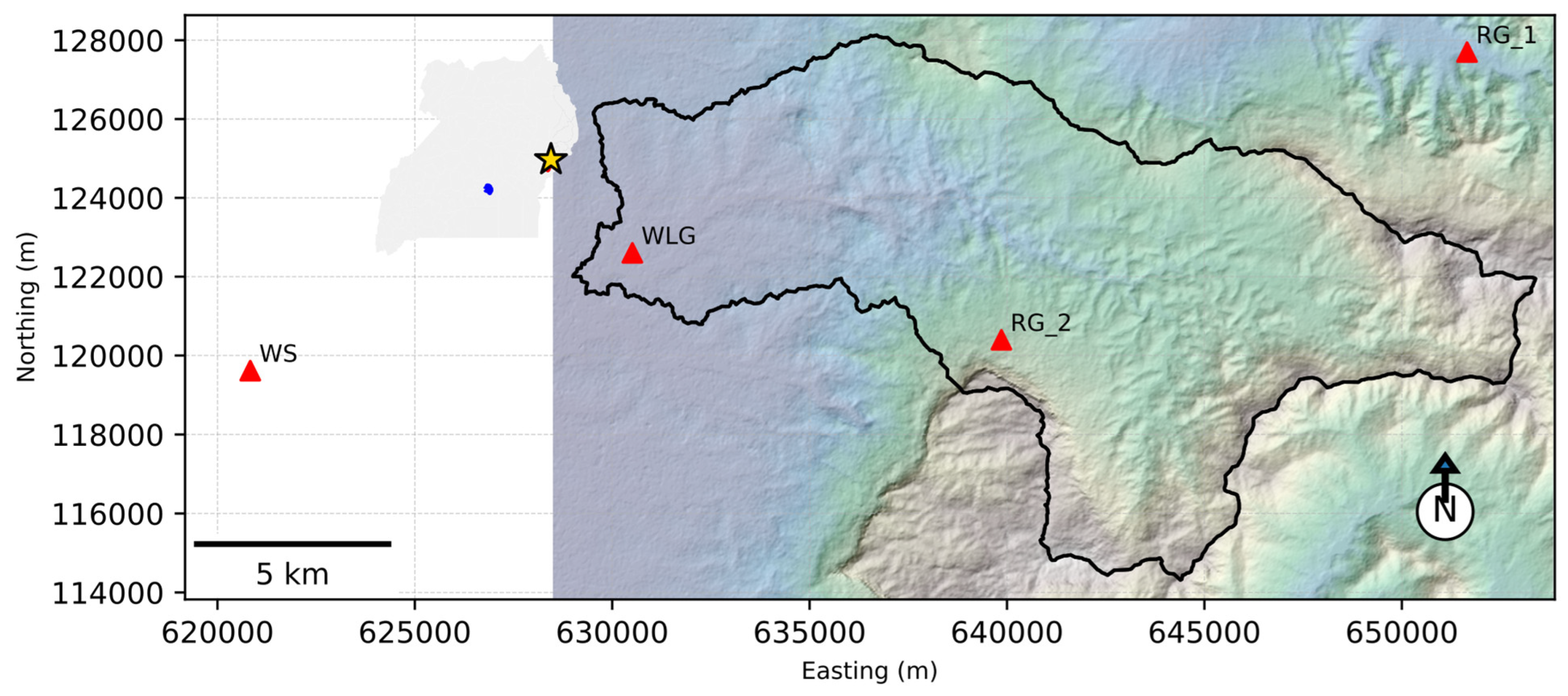
Figure 1. Map of Namatala River catchment. The main panel shows the catchment boundary—black line—draped over a hill-shade and terrain color relief derived from a DEM. Red triangles mark monitoring sites: RG_1 and RG_2 are rainfall gauges (rainfall only); WS is a meteorological station measuring rainfall, relative humidity, wind speed, air temperature, and incoming solar radiation; WLG is the water-level gauge located on the Mbale–Soroti Highway. The gold star in the inset locates the catchment within Uganda; the blue symbol shows Kampala, Uganda’s capital.
Hydrology 12 00309 g001
Figure 2. Conceptual framework of TopEros. Note that SRO refers to the surface runoff predicted by the hydrological model and EGEM represents the erosion model due to concentrated flow. Also note that we adopted the erosion risk ranges shown in Table 1.
Hydrology 12 00309 g002
Figure 3. Observed daily rainfall, observed daily hydrograph, and the daily hydrograph simulated by TOPMODEL. Panels (a,b) are as predicted in 2015 and 2016, respectively.
Hydrology 12 00309 g003
Figure 4. Like Figure 3 above, only for monthly streamflow time series. Panels (a,b) are as predicted in 2015 and 2016 respectively.
Hydrology 12 00309 g004
Figure 5. Daily predicted soil erosion by type and sediment deposition in Namatala River catchment as predicted by TopEros. Panels (a,b) are as predicted in 2015 and 2016, respectively.
Hydrology 12 00309 g005
Figure 6. Yearly grid-scale soil erosion of Namatala River catchment as predicted by TopEros. Panels (a,b) are as predicted in 2015 and 2016, respectively.
Hydrology 12 00309 g006
Figure 7. Same as Figure 6 above, only for sediment deposition. Panels (a,b) are as predicted in 2015 and 2016, respectively.
Hydrology 12 00309 g007
Figure 8. Erosion risk map of Namatala River catchment. Note that the values 0, 1, 2, 3, and 4 on the color bar correspond to Jiang et al.’s [39] very low, low, moderate, high, and very high classes, respectively (Table 1).
Hydrology 12 00309 g008
Table 4. Sediment yield, sediment deposition, and gross soil erosion as predicted by TopEros in Namatala River catchment. CSY is the sediment yield, CSD is the sediment deposition, CGE_Dof is catchment gross soil erosion by the sheet erosion process, CGE_Dr is catchment gross soil erosion by raindrop detachment, and CGE_Df is catchment gross soil erosion by concentrated flow.
YearCSY (Mgyr−1)
×106
CSD (Mgyr−1)
×106
CGE_Dof (Mgyr−1)
×106
CGE_Dr (Mgyr−1)CGE_Df (Mgyr−1)
×106
Model
20152.3874.1414.4382.5102.090TopEros
20152.9153.697MUSLE
20161.4433.1102.7141.7191.839TopEros
20161.7743.697MUSLE
Table 5. Soil erosion simulation in Namatala River catchment. Note that CSY is catchment-specific sediment yield, CSD is catchment-specific sediment deposition, SDR* is sediment delivery ratio from TopEros, and SDR** is the sediment delivery ratio from the empirical relationship of [59], as cited in [60,61].
YearCSY (Mgha−1yr−1)CSD (Mgha−1yr−1)SDR*SDR**Model
20151552700.3660.252TopEros
20151902410.4410.252MUSLE
2016942020.3170.252TopEros
20161151370.4560.252MUSLE
Disclaimer/Publisher’s Note: The statements, opinions and data contained in all publications are solely those of the individual author(s) and contributor(s) and not of MDPI and/or the editor(s). MDPI and/or the editor(s) disclaim responsibility for any injury to people or property resulting from any ideas, methods, instructions or products referred to in the content.