Abstract
Accurately estimating the time of concentration (Tc) is critical for hydrological modelling, flood forecasting, and hydraulic infrastructure design. However, conventional methods often overlook the combined effects of rainfall intensity and antecedent soil moisture, thereby limiting their applicability under changing climates. This study presents a novel approach that integrates data-driven techniques with remote sensing data to improve Tc estimation. This method was successfully applied in the Kalu River Basin, Sri Lanka, demonstrating its performance in a tropical catchment. While an overall inverse relationship between rainfall intensity and Tc was observed, deviations in several events underscored the influence of initial soil moisture conditions on catchment response times. To address this, a modified kinematic wave-based equation incorporating both rainfall intensity and soil moisture was developed and calibrated, achieving high predictive accuracy (calibration: R2 = 0.97, RMSE = 1.1 h; validation: R2 = 0.96, RMSE = 0.01 h). A hydrological model was developed to assess the impacts of Tc uncertainties on design hydrographs. Results revealed that underestimating Tc led to substantially shorter lag times and significantly increased peak flows, highlighting the sensitivity of flood simulations to Tc variability. This study highlights the need for improved estimation and presents a robust, transferable methodology for enhancing hydrological predictions and climate-resilient infrastructure planning.
1. Introduction
Time parameters play a crucial role in hydrological and hydraulic design, influencing a wide range of applications, including flood forecasting, early warning, reservoir operation, urban drainage planning, and watershed management [1,2]. Accurate determination of runoff response timing is essential for predicting peak discharges, estimating flood volumes, and generating realistic design hydrographs, which are critical elements in both real-time operations and infrastructure design [3,4,5,6]. In hydrological modelling, temporal characteristics play a critical role, particularly during the parameter calibration phase [7]. Inaccurate representation of runoff timing, stemming from erroneous assumptions regarding time-dependent parameters, is likely to lead the calibration process to converge on parameter sets that may yield statistically acceptable performance but lack physical realism or hydrological plausibility [2,8]. Such discrepancies undermine the model’s robustness and compromise its predictive reliability, particularly in operational forecasting applications and in data-scarce environments where opportunities for model validation are limited [9,10].
Among various time-related parameters, the time of concentration (Tc) is one of the most widely used and referenced, serving as a proxy for the watershed response time and forming the basis for many empirical and conceptual modelling approaches [1]. In its International Glossary of Hydrology, the World Meteorological Organisation defines Tc as the time required for storm runoff to travel from the most hydraulically remote point of a drainage basin to its outlet [11]. Although multiple definitions of Tc have been proposed in the literature [1], the most widely applied approach remains the one based on the distance along the principal flow path and corresponding flow velocity. This method is extensively used in hydrological modelling, including in widely used numerical models such as the Hydrologic Engineering Center’s Hydrologic Modelling System (HEC-HMS) [7]. Beyond this theoretical definition, the literature presents multiple interpretations of Tc and related time parameters of hydrographs, such as lag time and time to peak, which are conceptually linked to Tc [1,7].
McCune [12] identified six different methods for estimating (computational definitions) Tc using observed river discharge (or direct runoff) and rainfall (or excess rainfall), reflecting the diverse approaches employed in hydrological analysis. In contrast, Beven [13] argues that Tc should be estimated using surface, subsurface, and channel flow celerities rather than flow velocities. Several studies have employed particle-tracking methods to estimate the travel time of overland flow, particularly on impervious surfaces, by simulating the movement of individual water particles along the flow path [14]. Beyond these approaches, numerous empirical formulas have been developed to estimate hydrograph time parameters, particularly for ungauged catchments where direct measurements are unavailable [4,15,16,17,18,19]. These formulas commonly incorporate catchment area, overland flow length, and slope, whether of the main channel or the average watershed, underscoring their reliance on fundamental watershed characteristics [20]. Several studies have also taken into account the effects of land use development on time parameters. These include the use of Manning’s roughness coefficient [21,22], imperviousness factors [23,24,25], and conveyance factors that consider the hydraulic characteristics of the flow channel [26,27]. Gericke and Smithers [28] provided a comprehensive review of three hydraulic and 44 empirical or semi-analytical formulas used to estimate key time parameters, including time of concentration, lag time, and time of rise.
Early studies also considered meteorological influences on hydrograph timing parameters by incorporating rainfall intensity into their estimations. For instance, Morgali and Linsley [21] conducted a sensitivity analysis using a dynamic-wave overland flow model, where rainfall intensity was a key variable used to examine its effect on the shape and timing of runoff hydrographs. Several subsequent studies included the critical rainfall intensity, corresponding to a duration equal to the time of concentration, as an independent variable, introducing a circular dependency in estimating Tc. To resolve this, an iterative solution method was applied until convergence for Tc is achieved [26]. Several field studies and laboratory experiments [29,30,31] have also confirmed the importance of rainfall intensity in accurately estimating time of concentration, using a range of land uses, catchment sizes, and rainfall conditions.
Despite accounting for meteorological factors, many empirical methods for estimating Tc fail to represent catchment dynamics accurately. Among the widely used approaches, only the NRCS (National Research Conservation Service) method partially incorporates these dynamics through the Runoff Curve Number (CN), which indirectly reflects soil moisture by considering factors such as hydrologic soil group (A, B, C, and D, with decreasing infiltration capacity from A to D), land use and land cover (e.g., urban, cultivated agricultural, other agricultural, and arid or semi-arid rangelands), and antecedent runoff conditions [32]. However, no widely adopted Tc estimation method explicitly includes soil moisture as a dynamic variable, revealing a critical gap in accurately capturing the temporal response of catchments.
Soil moisture is a critical determinant of watershed hydrology, exerting a direct influence on infiltration, runoff generation, flow velocity, and, consequently, the time of concentration [3,4]. When antecedent soil moisture is high and infiltration is limited, it results in increased surface runoff and higher flow velocities, as well as a decreased time of concentration. Incorporating soil moisture into Tc estimation is therefore essential for improving the accuracy of catchment response time, particularly in regions with high spatial and temporal fluctuations of soil moisture.
There are two methods for measuring soil moisture: in situ measurements and remote sensing measurements. Although in situ measurements are continuous and accurate, their limited spatial coverage makes them ineffective in representing regional soil moisture conditions within large river basins [33,34]. Remote sensing soil moisture (RSSM) measurements, on the other hand, provide extensive spatial coverage [34]. Currently functioning RSSM products, such as the Soil Moisture and Ocean Salinity (SMOS), launched by the European Space Agency (ESA), and Soil Moisture Active Passive (SMAP), launched by the National Aeronautics and Space Administration (NASA), have improved algorithms for surface soil moisture inversion and a larger soil penetration depth. However, they are less sensitive to the influence of vegetation structure, surface roughness, snow cover, frozen soil, and precipitation events due to their poor spatial resolution [35]. The SMAP Level 4 (SMPA L4) mission provides both surface soil moisture data (at ~5 cm depth), and root zone soil moisture data (at ~100 cm depth) at three-hourly temporal and 9 km × 9 km spatial resolution, while SMOS provides surface soil moisture data at 3-day intervals with much coarser (35–50 km) spatial resolutions. Pabasara et al. [36] have illustrated the successful integration of SMAP L4 root zone soil moisture data in enhancing the performance of a hydrological model through multi-variable calibration with streamflow and soil moisture, for the data-scarce Maduru Oya river basin in the dry zone of Sri Further, SMAP L4 data have been successfully utilised in the modification of the Combined Drought Index (CDI) framework by replacing the snow cover component with root-zone soil moisture derived from SMAP L4 data, making it more suitable for rain-fed catchments where soil moisture plays a critical role in drought dynamics [37].
In recent years, the growing impact of climate change has underscored the crucial need for a thorough understanding of hydrological processes, notably rainfall intensity changes and their temporal implications on watershed dynamics. At the global/regional scales, the consequences of altered precipitation patterns are increasingly evident, with significant implications for ecosystems and water resources [38]. While several traditional methods exist for estimating the time of concentration (), such as the NRCS Soil Conservation Service (SCS) method, they often assume static watershed and rainfall conditions and therefore may not fully capture event-specific variability. In response to these challenges, this study focuses on two complementary objectives: the development of a novel methodology that establishes a dynamic relationship between rainfall intensity and , further enhanced by incorporating soil moisture, and the application of this methodology to the Kalu River Basin in Sri Lanka as a case study to evaluate its hydrological implications. Accordingly, the study compares uncertainties in streamflow dynamics due to Tc estimations (viz., the conventional NRCS Soil Conservation Service (SCS) method and the proposed novel approach) using a HEC-HMS-based hydrological model developed for the tropics of Kalu River Basin, Sri Lanka, to assess their impact on the design hydrograph.
2. Materials and Methods
This section is organised into multiple sub-sections. First, the study area is described, followed by an overview of hydro-meteorological and remote sensing data collection and preprocessing. Next, the selection of representative rainfall events for evaluating the Tc estimation technique is summarised. The estimation of Tc using the Detrending Moving-average Cross-correlation Analysis (DMCA) approach is subsequently presented. To address the limitations associated with the DMCA-based Tc estimation, the integration of soil moisture into the modelling approach is then elaborated. Finally, to evaluate the uncertainties associated with the Tc estimation method in streamflow simulation, the development of the Hydrological Model using HEC-HMS is discussed.
2.1. Study Area
The Kalu River, located entirely in the wet zone of Sri Lanka, spans ~100 km in length and drains a catchment area of about 2816 km2 (Figure 1) to the Indian Ocean. Despite being the third-longest river in the country, the Kalu River has the highest annual discharge, draining more than 4000 Million Cubic Meters (MCM) of water each year [39]. The entire basin receives an average annual rainfall of ~4000 mm, with significant spatial variability, ranging from ~6000 mm in mountainous regions to ~2000 mm in lowland plains [40].
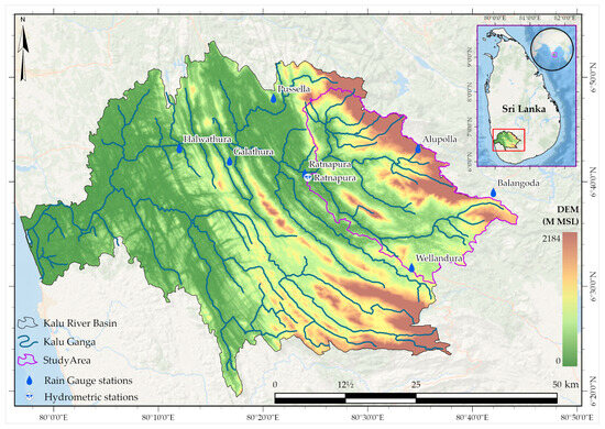
Figure 1.
Ratnapura sub-basin of Kalu River Basin.
The stretch from its source to Ratnapura (Ratnapura sub-watershed, Figure 1) features a narrow bed and steep banks, descending from 2250 m to 14 m above sea level over 36 km. After merging with the Wey River at Ratnapura, it continues for another 76.5 km before reaching its outlet at Kalutara. Due to its steeper terrain and high rainfall in the upstream Ratnapura sub-watershed (drainage area of 603 km2), the lower floodplain experiences frequent flooding, particularly during the May to September South-West Monsoon period. The South-West Monsoon period accounts for ~51% of the annual rainfall in the Ratnapura sub-watershed, making it the season with the highest rainfall [41]. The First Inter-Monsoon (March to April) and the North-East Monsoon (December to February) account for about 13% and 14% of its annual rainfall, respectively, while the Second Inter-Monsoon (October to November) brings around 22% [41] of the yearly precipitation. The annual average maximum and minimum temperatures in this region are ~32 °C and ~23 °C, respectively. Figure A1 illustrates the intra-annual variability of the precipitation at all the relevant stations. Most of the basin area is covered with trees (~53%), while the rangeland (~16%), crops (~14%), built-up area (~14%), and water bodies (~3%) are the other dominant land-cover classes of the Kalu River Basin. Figure A2 shows the land use/land cover map of the basin. The prominent soil type is Clay-rich Acrisol, which covers ~98% of the basin area.
2.2. Hydro-Meteorological and Remote Sensing Data Collection & Preprocessing
The hydro-meteorological data required for estimating Tc were obtained from the Department of Meteorology (rainfall data) and the Irrigation Department (streamflow data) in Sri Lanka. Hourly rainfall and streamflow data at the Ratnapura stations (Table A1 and Table A2) were collected. For the Alupola, Balangoda, and Wellandura stations (Table A2), only daily rainfall data were available; therefore, hourly rainfall series were derived by applying the temporal distribution pattern observed at the Ratnapura station, assuming similar intra-day rainfall variability [42,43]. As all rainfall and streamflow records were complete without missing data, the datasets were directly used to identify the representative rainfall events for the study.
Notably, the Tc estimation technique employed in this study does not require continuous records to yield robust estimates, despite being a time series analysis. In cases where data gaps are present, this method is capable of automatically estimating Tc using other continuous segments of the record, thereby reducing the need for extensive data preprocessing [44]. However, this becomes invalid whenever the data becomes highly intermittent; for instance, missing one hourly timestep per day, as excessive segmentation can compromise the accuracy of the Tc estimates. To ensure reliability, the time series dataset should include at least one continuous segment without missing time steps longer than the maximum moving average window length (L) tested [44].
To assess the impact of antecedent soil moisture conditions on the Tc, surface soil moisture data from the SMAP L4 product, which is available at a 9 km × 9 km spatial resolution and 3 h temporal resolution, were used in this study. The relevant SMAP L4 retrievals for the Ratnapura subbasin were extracted using the Google Earth Engine platform. To accommodate the lumped behaviour of the watershed at a daily timestep, the SMAP-L4 retrievals were spatially and temporally averaged. Furthermore, a Digital Elevation Model (DEM) was obtained from the United States Geological Survey (USGS) Earth Explorer tool and used to delineate the catchment and the river network. The summary of the hydro-meteorological and remote sensing data utilised in this study is presented in Table 1.

Table 1.
Summary of the hydro-meteorological and remote sensing datasets used in this study.
2.3. Event Selection
Several rainfall events, representing three categories of daily rainfall intensities (viz., extreme, moderate, and low), were selected from the period March 2015 to July 2023 to evaluate the proposed Tc estimation methodology (Table 2). This classification scheme facilitates a systematic assessment of rainfall variability and the characterisation of precipitation extremes. In this dataset, extreme events correspond to rainfall intensities exceeding the 98th percentile, amounting to more than 136 mm/day. The moderate events fall within the 60th and 80th percentile range, with intensities between 41 mm/day and 55 mm/day. The low-intensity events are defined within the 30th and 40th percentile range, with intensities between 28 mm/day and 32 mm/day [45,46,47].
Table 2.
Event Selection Based on Percentiles.
2.4. Estimating Time of Concentration—DMCA-Based Approach
For the initial Tc estimation procedure, the data-driven Detrending Moving-Average Cross-Correlation Analysis (DMCA) technique, which utilises rainfall and streamflow time series, was employed. Developed initially in the field of economics to identify the time scale of the strongest correlation between two variables [48,49], the DMCA technique can be applied in hydrology to determine the characteristic timescale over which a noisy rainfall input is transformed into a smoother streamflow response at the catchment outlet [44,50]. The key advantage of the DMCA method is its ability to identify the correlation between time series that may have different frequency spectra and exhibit nonlinear relationships. In contrast, the conventional cross-correlation analysis requires prior smoothing of the rainfall series to match the frequency characteristics of streamflow. Such preprocessing can distort the original structure of the rainfall signal, potentially introducing inaccuracies and undermining the inherent catchment characteristics in estimating the catchment response time (). DMCA overcomes this limitation by analysing the intrinsic correlation structure without altering the original time series [47,50].
In this study, the catchment response time () was first estimated using the DMCA method. Subsequently, Tc was derived using the empirical relationship given by Equation (1) [20]:
The analytical procedure for estimating the response time () using the DMCA-based technique involves a structured sequence of steps. This method is applied to hourly rainfall and streamflow time series and can be described as follows for a given rainfall event.
At first, a cumulative time series of rainfall Rₜ and streamflow Qₜ is created for each selected occurrence, over a common duration T (in hours), using an identical (hourly) time step. These were defined as Equations (2) and (3):
where and denote the rainfall and streamflow values at time i in hours.
Then, for a single moving average window length (L), the deviations (fluctuations) of each cumulative time series are compared to its centred moving average with window length (L), where L is an odd integer expressed in hourly time steps. This process is referred to as detrending. The purpose of detrending was to isolate the correlation structure and to eliminate non-stationary trends. Then, the mean-squared fluctuations as and for rainfall and streamflow, respectively, are calculated as in Equations (4) and (5).
and are the centred moving averages of the cumulative rainfall and streamflow, respectively, with moving average window length (L) at time t, as in Equations (6) and (7).
Similarly, the mean squared value of the bivariate fluctuations between the cumulative rainfall and streamflow time series (Equation (8)) was computed:
Finally, the DMCA-based correlation coefficient corresponding to the selected window length L, , which measures the intensity and direction of the connection between rainfall and streamflow for a given L (9) was calculated:
Here, a wide range of moving average window lengths (L), ranging from 3 h to several days, was tested to explore the relationship between rainfall and streamflow across varying temporal scales. The window length (L) was incremented in 2 h steps to ensure that all window lengths remained odd integers. This choice strikes a balance between temporal resolution and the ability to detect key hydrological patterns, particularly those associated with short-duration, high-intensity rainfall events. It also serves as a compromise between filtering out high-frequency noise and preserving critical hydrological signals. While shorter windows may fail to capture essential dynamics, excessively long windows can introduce unwanted noise [44,50].
In this study, the DMCA method is adapted in a hydrological context and reinterpreted to derive a quantitative estimate of the catchment response time (). Specifically, the optimum window length (Lmin) that yields the minimum DMCA-based correlation coefficient () is identified for each event. This minimum correlation indicates the weakest statistical dependency between rainfall and streamflow, thereby providing the most unambiguous indication of the time lag between them. This optimum window length (Lmin) generally corresponds to approximately twice the actual time lag (Tp), effectively aligning the second half of the rainfall event with the first half of the streamflow response. The catchment response time (), conceptually similar to the time lag (Tp) (NRCS, 1986), is then estimated as half of (Lmin—1), following the reinterpretation proposed by Giani et al. [44,50]. This approach thereby introduces a novel use of the DMCA method for hydrological analysis.
2.5. Improving Time of Concentration Estimation: Integrating Soil Moisture
The empirical kinematic wave formula was adopted and extended to quantitatively integrate the influence of soil moisture dynamics on Tc estimations. The conventional form of Equation (10), proposed by McCuen et al. [26], estimates Tc based on catchment characteristics and rainfall intensity. In this study, the equation was modified to include soil moisture (SM) as an additional explanatory variable, resulting in a more dynamic formulation (Equation (11)) capable of capturing variation in flow response driven by both rainfall and antecedent soil moisture conditions. In particular, for each selected rainfall event, the mean soil moisture content on the day before the event was used to represent the catchment’s antecedent wetness condition. The rainfall intensity used in the formulation was estimated by spatially averaging measured rainfall using the Thiessen Polygon method and temporally averaging it with the arithmetic mean method over the total rainfall duration. Thus, the current experimental model based on the kinematic wave formula (10) was extended to account for the soil moisture effect through Equation (11).
where Tc is the time of concentration (hours), L is the length of the main channel (m), n is the Manning’s roughness coefficient, i is the rainfall intensity (mm/hr), SM is the soil moisture (m3/m3), and S is the catchment slope (m/m).
The modified Equation (11) includes six unknown parameters: C, a, b, c, d, and e. To identify these parameters, nonlinear regression analysis was implemented in Python (version 3.10), incorporating observed data from 10 rainfall events and the respective Tc estimates obtained from the DMCA method, under model calibration. The remaining events were used for model validation. The optimisation process was structured to ensure that the resulting equation realistically represented hydrological behaviour, such as the inverse connection between rainfall intensity and Tc, while also capturing the influence of antecedent soil moisture.
2.6. Hydrological Modelling—HEC-HMS
The HEC-HMS model is a semi-distributed hydrological model that combines both physical and conceptual modelling approaches, offering considerable flexibility for simulating streamflow across various geographical settings. Given that Tc directly affects the simulations, this study developed an HEC-HMS model to represent two selected rainfall events, evaluating the impact of uncertainties in Tc on design hydrograph estimation. The hydrological model was configured to compare the conventional NRCS-SCS method with the newly modified kinematic wave equation method. To isolate the influence of Tc, only the lag time parameter was varied between the two events while keeping all other model settings identical. The analysis was performed using two representative rainfall events: 15–17 May 2020, for calibration, and 31 August to 3 September 2022, for validation.
Model performance was assessed using four widely used objective functions: Nash-Sutcliffe Efficiency (NSE) and Percent Bias (PBIAS), to ensure a comprehensive evaluation of the hydrograph estimations [51]. NSE determines the relative magnitude of the residual variance compared to observed variance and is highly sensitive to high flows with an optimal value of 1.0. PBIAS measures the biases between simulated and observed flows. The optimal value of PBIAS is zero, and overestimations and underestimations are denoted by positive and negative values, respectively. Root Mean Square Error (RMSE) indicates the errors in simulation, with an optimal value of 0. The Coefficient of Determination (R2) describes the collinearity between simulated and observed data, with an optimal value of 1.0.
The modelling framework is summarised and presented in the following methodology flowchart (Figure 2).
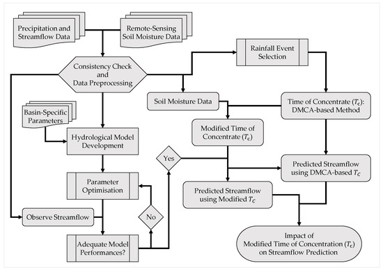
Figure 2.
Methodology flowchart.
3. Results
This section is organised into three sub-sections. The first presents the results of the DMCA-based time of concentration (Tc) estimation method and its relationship to averaged rainfall intensity. The second sub-section details the integration of SMAP L4 soil moisture data into the Tc estimation process, addressing the limitations of conventional methods in capturing dynamic catchment conditions. The third sub-section evaluates the uncertainties introduced in the design hydrograph due to variations in Tc, comparing outcomes from both the conventional NRCS-SCS approach and the proposed soil moisture-integrated method.
3.1. DMCA-Based Time of Concentration Estimation
The analysis of rainfall intensity over the study period revealed a total of five extreme rainfall events, fifteen moderate events, and four low-intensity events (Table 2). Notably, the standard deviation of rainfall amounts across these categories highlights a significant disparity in variability, with extreme events exhibiting the highest variation (44.4 mm), followed by moderate (3.7 mm) and low-intensity events (1.4 mm) (Figure 3). This elevated variability in extreme rainfall events can be attributed to their random and infrequent occurrence. Unlike moderate and low-intensity rainfall, which tend to occur more frequently under relatively stable atmospheric conditions, extreme events are typically driven by highly dynamic and localised meteorological phenomena such as convective storms, tropical depressions, or monsoonal surges. These three rainfall intensity categories are expected to generate markedly different catchment responses due to their influence on the time of concentration.
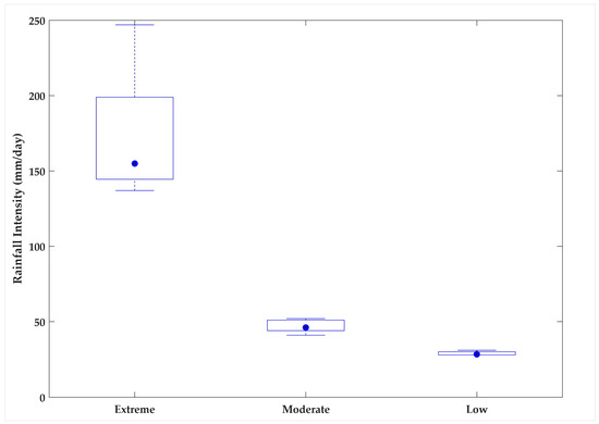
Figure 3.
Variation in rainfall intensity among the three selected rainfall categories. The boxes are limited to the 25th and 75th percentiles, and the dots show the median (i.e., 50th percentile) values of the respective datasets. Whiskers are extended to 1.5 times the inter-quartile range to the top and bottom of the boxes.
Figure 4 illustrates the application of the DMCA method to rainfall and streamflow time series for three selected events representing extreme, moderate, and low rainfall categories. It also includes the moving average of the cumulative time series based on the optimal window length. In the cumulative rainfall time series, steeper gradients indicate intense rainfall occurring over a short duration, characteristic of extreme rainfall events, whereas flatter sections correspond to periods of low or no rainfall. Similarly, the cumulative streamflow time series for extreme events displays a steep slope, reflecting a rapid catchment response. In contrast, moderate and low-intensity rainfall events exhibit gentler gradients, indicating slower runoff generation and a more delayed hydrological response. The optimal window length (Lmin) that yields the minimum DMCA-based correlation coefficient was estimated for each event. The results show that both Lmin and the corresponding time lag are generally shorter for extreme rainfall events, while moderate and low-intensity events tend to produce longer Lmin values and time lags (Table 3). Similarly, time lags were estimated for all 24 rainfall events and analysed in terms of the average rainfall intensity.
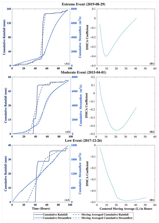
Figure 4.
Application of the DMCA method to rainfall and streamflow time series for three selected events representing extreme, moderate, and low rainfall categories.
Table 3.
Variation in rainfall intensity with DMCA-derived time lag and time of concentration for three selected rainfall events.
The study of all 24 chosen rainfall events, classified as extreme, moderate, or low intensity, offers a more comprehensive understanding of the relationship between rainfall intensity and Tc estimated by the DMCA-based approach. Figure 5 presents a scatter plot of rainfall intensity versus Tc, illustrating the overall trend and clearly establishing the theoretically expected inverse relationship: higher rainfall intensities generally result in lower Tc values. Most high-intensity events exhibited relatively short Tc values, reflecting rapid hydrological response to intense rainfall. In contrast, lower-intensity events tended to produce longer Tc values, suggesting that the rainfall was insufficient to generate quick or significant runoff.
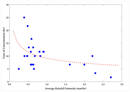
Figure 5.
Relationship between rainfall intensity and DMCA-derived time of concentration (Tc). The dashed red line shows the best fit to the dataset.
However, notable deviations from this trend were observed, particularly among some moderate and low-intensity events. Additionally, a few high-intensity events produced unexpectedly high Tc values, resulting in a low coefficient of determination (R2 = 0.4) for the fitted exponential relationship. Despite these anomalies, the general trend supports the theoretical expectation of an inverse relationship between rainfall intensity and Tc. These outliers highlight a critical need to improve Tc estimations by potentially accounting for additional factors, such as antecedent soil moisture or land surface conditions.
3.2. Refining Rainfall Intensity-Time of Concentration Relationships Through SMAP Soil Moisture Data
Certain deviation points in Figure 5 suggest that rainfall intensity alone may not be sufficient to explain catchment response times. Specifically, several high-intensity rainfall events had unexpectedly large Tc values, showing potential limitations of the DMCA-based approach in accurately representing the catchment’s hydrological behaviour. Several moderate-to-low-intensity rainfall events had considerably lower Tc values, outperforming the conventional notion of the inverse relationship between rainfall intensity and Tc. These unusual results suggested that factors more than just rainfall intensity, such as antecedent soil moisture conditions, could play a significant role in influencing how quickly the catchment responds. To explore this issue further, remotely sensed soil moisture data from NASA’s Soil Moisture Active Passive (SMAP) mission were incorporated into the modelling approach. Figure 6 shows the daily averaged soil moisture data for the day before each rainfall event used to capture the catchment’s wetness conditions prior to the rainfall.
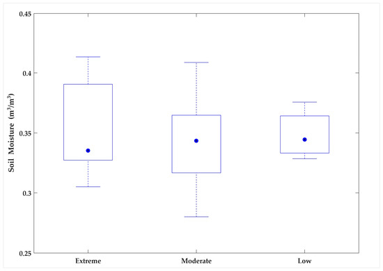
Figure 6.
Daily averaged soil moisture on the day prior to each rainfall event. The boxes are limited to the 25th and 75th percentiles, and the dots show the median (i.e., 50th percentile) value of the respective soil moisture datasets. Whiskers are extended to 1.5 times the inter-quartile range to the top and bottom of the boxes.
The SMAP-derived soil moisture data show significant changes in antecedent moisture levels among the three rainfall categories. These findings suggest that antecedent soil moisture is an important component in determining the intensity of rainfall events, which has significant implications for runoff generation and catchment behaviour. This allows for the assessment of whether adding soil moisture as an extra variable could improve the estimation of Tc across various rainfall events.
The model’s performance was much improved by the modified Equation (12), which included soil moisture. According to statistical analysis, the new model accounted for 97% of the variance in Tc across the observed occurrences, with a coefficient of determination (R2) of 0.97 and a Root Mean Square Error (RMSE) of 1.1 h. When compared to the initial DMCA-based relationship between Tc and rainfall intensity, these performance indicators show a significant improvement in accuracy.
Additionally, the incorporation of soil moisture corrected previously inconsistent Tc values, which had been affected by higher rainfall intensities, resulting in longer estimates. Low antecedent soil moisture prior to an extreme rainfall event tended to produce comparatively longer Tc values, likely due to the initial infiltration capacity delaying the generation of surface runoff. In contrast, high antecedent soil moisture preceding moderate or even low-intensity rainfall events often resulted in shorter Tc values, as the catchment was already saturated, leading to quicker surface runoff and faster hydrological response. Consistent with hydrological theory, the revised model demonstrated a continuous and consistent negative relationship between rainfall intensity and Tc. Figure 7 presents a comparison between the original and modified Tc estimates, clearly illustrating the correction of earlier discrepancies and the overall improvement in the reliability of Tc estimation. Accordingly, the following section presents a comparison of the uncertainty associated with estimating peak flow and the design hydrograph when using the conventional NRCS-SCS equation versus the modified Tc equation, which incorporates the effects of rainfall intensity and soil moisture.
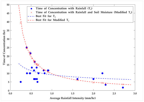
Figure 7.
Comparison of results with and without the effect of soil moisture.
3.3. Comparison of Hydrograph Responses Using Conventional and Modified Tc Approaches
To assess the practical implications of accurately representing time of concentration (Tc) in hydrological modelling, two rainfall events were simulated in HEC-HMS using Tc values estimated by both the conventional NRCS-SCS equation and a modified approach that incorporates rainfall intensity and soil moisture. Calibration and validation of HEC-HMS parameters were carried out, and the details are provided in Table A3. For example, initial abstraction, representing canopy and surface losses, was estimated using the SCS Curve Number method as 0.2 times the potential maximum retention, while the initial baseflow discharge was determined from observed river discharge prior to the rainfall events. The initial Curve Number (CN) was assigned based on land use and soil type in the study area, with minor adjustments introduced during model calibration and validation. These parameters were then kept constant across simulations with different Tc values, ensuring that variations in the results can be explicitly attributed to the Tc formulations rather than to inconsistencies in model parameterisation. Using the Tc estimated by the NRCS-SCS method, the optimised parameter set (Table A3) for the calibration event (15–17 May 2020) demonstrated strong agreement between simulated and observed flows (Figure 8), with a Nash–Sutcliffe Efficiency (NSE) of 0.87, a PBIAS of 6.6%, and a simulated peak discharge of 163 m3/s compared to the observed 167 m3/s. For the validation event (31 August–3 September 2022), the same parameter set yielded an NSE of 0.91 and a PBIAS of −6.9%, with the simulated peak discharge of 272 m3/s closely matching the observed value of 270 m3/s.
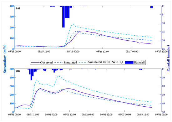
Figure 8.
Changes in design hydrographs with time of concentration for calibration (A) and validation (B) events.
Although the conventional Tc estimation method may optimise model parameters to yield statistically satisfactory results for specific calibration and validation events, these parameters may not be physically realistic when applied to rainfall events with different magnitudes or characteristics. The Tc value estimated using the NRCS-SCS method is based solely on catchment physical characteristics and therefore remains constant at 255 min. However, when the effects of rainfall intensity and soil moisture are incorporated, the estimated Tc values are reduced by 37% and 44% for the calibration and validation events, respectively. As a result, the newly computed lag times of 143 and 160 minutes led to significant changes in simulated hydrograph characteristics, producing earlier and more pronounced peak flows of 415 m3/s and 231 m3/s, respectively, as shown in the hydrographs (Figure 8). These outcomes are summarised in Table 4.
Table 4.
Summary of hydrological modelling.
This comparison demonstrates how changes in Tc estimation influence the accuracy and reliability of hydrological model outputs. By examining changes in peak flow, time to peak, and overall hydrograph shape, the analysis underscores that conventional Tc values, although capable of producing statistically acceptable simulations, may not reflect the actual temporal dynamics of runoff generation. This finding reinforces concerns raised in earlier studies about the risk of calibrating model parameters under incorrect temporal assumptions [2,8,13].
3.4. Sensitivity Analysis
The sensitivity analysis reveals distinct responses of the time of concentration () to variations in the key parameters (Figure 9). Manning’s roughness coefficient (n) and channel length (L) show nearly linear positive relationships with , where a 50% increase in n and L results in increases of ~34% and ~26% in , respectively. In contrast, catchment slope (S) exerts an opposite influence: increasing S by 50% reduces by ~25%, while decreasing S substantially increases (up to ~64%), highlighting its strong control on flow velocity. Soil moisture (SM) demonstrates a moderate effect, with a 50% decrease in raising by ~25%, whereas increased SM slightly reduces . Rainfall intensity (i) emerges as the most sensitive factor, where a 50% reduction causes to more than double (~103%), while a 50% increase shortens by ~34%. These results emphasise that is highly sensitive to rainfall intensity and slope, while roughness, channel length, and soil moisture exert secondary but notable influences.
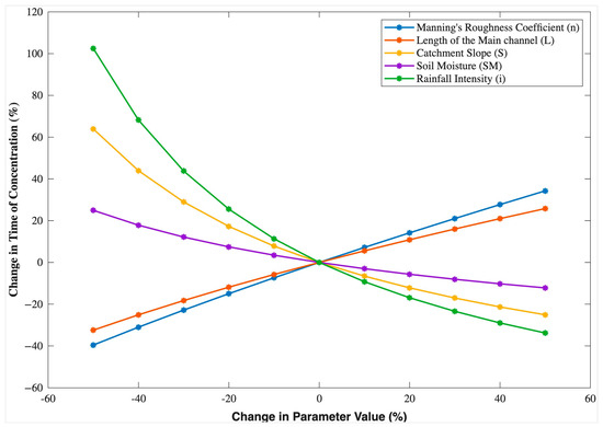
Figure 9.
Sensitivity of time of concentration () to ±50% changes in Manning’s roughness coefficient (n), channel length (L), catchment slope (S), soil moisture (SM), and rainfall intensity (i).
4. Discussion
Early studies on Tc estimation often relied on long-term or generalised rainfall characteristics, which may not adequately reflect the temporal variability and dynamics of individual storm events. For instance, Schmidt and Schulze [52] proposed modified SCS lag equations based on parameters such as mean annual precipitation and rainfall intensity associated with specific return periods. Similarly, McCuen et al. [26] used the 2-year rainfall intensity over a duration equal to Tc itself, a method that assumes uniform storm characteristics and overlooks variability in rainfall structure across different events. While these approaches provided improved estimations of Tc compared to the standard SCS lag equation, they are unable to capture event-specific catchment responses influenced by real-time rainfall dynamics. The findings of our study emphasise the importance of using actual event-based rainfall intensities in Tc estimation, as they better represent the magnitude of the specific rainfall event that drives runoff processes.
Around the same time, Kadoya and Fukushima [53] recognised the importance of using rainfall characteristics specific to individual events, particularly through the use of effective rainfall intensity to better represent runoff-generating potential. This approach was further supported by Fang et al. [54], who also utilised effective rainfall intensity to refine the estimation of time-related parameters such as Tc. Gericke and Smithers [28] adopted a similar event-focused perspective by incorporating average design rainfall intensity into their methodology. In addition to rainfall intensity, these studies emphasised the significance of antecedent soil moisture conditions, which influence both the volume and timing of runoff generation.
Although not always addressed explicitly, some studies have incorporated the effects of soil moisture indirectly in estimating the time of concentration (Tc). For instance, Simas [55] proposed a lag time estimation approach that uses the runoff Curve Number (CN), which inherently reflects the influence of land use, soil type, and antecedent soil moisture conditions. While such methods acknowledge the hydrological role of soil moisture, they do so through empirical parameters rather than direct physical representation. In contrast, the method proposed in this study explicitly integrates both event-specific rainfall intensity and antecedent soil moisture conditions, offering a more direct and physically meaningful approach to Tc estimation.
The estimation of design hydrographs, particularly peak discharge, is subject to significant uncertainty arising from inaccurate representation of catchment response times. Several studies have quantified the sensitivity of peak discharge to errors in time parameter estimation. For instance, Bondelid et al. [56] reported that up to 75% of the total error in peak discharge estimates can be attributed to inaccuracies in time parameter estimation. Similarly, McCuen [12] highlighted that when Tc is estimated based solely on channel characteristics, ignoring overland flow effects such as catchment roughness and slope, it tends to be underestimated by approximately 50%, leading to peak discharge overestimations between 30% and 50%. Gericke and Smithers [28] further demonstrated that errors in Tc estimation, ranging from underestimations of 20–65% to overestimations up to 700%, could result in corresponding peak discharge errors from +30% to −90%, underscoring the magnitude of this issue. Against this backdrop, the method proposed in this study reduces such uncertainties by directly incorporating catchment-specific, dynamic parameters such as event-based rainfall intensity and antecedent soil moisture content. The integration of these factors into the Tc estimation framework provides a more physically meaningful and event-responsive approach. Given the high sensitivity of peak discharge to Tc, as shown in previous studies, improving Tc estimation by incorporating rainfall intensity and soil moisture can help reduce the risk of deriving unrealistic optimised parameters and improve the overall consistency of hydrological design inputs.
However, it is essential to recognise that even when physically meaningful parameters such as rainfall intensity and antecedent soil moisture are integrated into the Tc estimation framework, their effectiveness depends on how they are applied within the hydrological modelling process. In this study, the initial parameter set in HEC-HMS was calibrated using a value derived from a conventional method (NRCS-SCS), which produced simulated streamflow that was in good statistical agreement with observed discharge. When the newly developed Equation (11), which incorporates event-specific rainfall intensity and antecedent soil moisture, was applied within the same calibrated model; however, the resulting peak flow and lag time deviated from the observed values. This outcome demonstrates that a single parameter set may not universally represent varying values. It also emphasises that while multiple parameter sets can generate acceptable statistical fits, they may differ in terms of physical realism. Therefore, to enhance the robustness and transferability of hydrological models, especially under changing climatic or land use conditions, it is essential to adopt multi-variable parameter calibration approaches [38]. Such methods can ensure that model parameters are not only statistically optimised but also hydrologically consistent with the dynamic behaviour of the catchment.
The proposed methodology builds upon established formulations that incorporate land use type, catchment scale, and topographic characteristics. Specifically, in Equation (11), parameters ‘n’, ‘L’, ‘S’, and ‘i’ represent land use, catchment size, topographic variation, and meteorological influences, respectively. The newly added parameter ‘SM’ further captures the effect of soil and land use through soil moisture. Nevertheless, the empirical constants (a–e) in Equation (11) are determined through statistical best fits and are thus likely to differ among river basins, suggesting the necessity of site-specific calibration when applying the model to diverse geographical and climatic settings. While groundwater dynamics may influence long-term hydrological responses, they are generally considered to operate on slower timescales than surface runoff and are thus unlikely to have a substantial impact on the time of concentration estimations presented in this study.
5. Conclusions
This study investigated the relationship between rainfall and catchment dynamics in Tc estimations through a DMCA-based approach and a newly developed equation that integrates soil moisture, while assessing the uncertainty in Tc estimation in hydrological modelling. The DMCA-based approach confirmed the general inverse relationship between rainfall intensity and Time of Concentration (Tc), where higher rainfall intensities result in faster catchment responses and hence shorter Tc. However, Tc estimations for several moderate- and low-intensity events deviated from this general trend, emphasising the potential influence of additional hydrological factors, such as antecedent soil moisture. Thus, the kinematic wave formula was modified to incorporate antecedent soil moisture, thereby addressing the limitations of the initial DMCA-based approach. The improved empirical kinematic wave equation performed better in Tc estimations, yielding correlation coefficients (R2) of 0.97 and 0.96 and root mean square errors (RMSE) of 1.1 and 0.01 h during calibration and validation events, respectively.
The performances of modified Tc and its consequent impact on streamflow prediction were evaluated using the HEC-HMS hydrological model. Our results highlight the sensitivity of the hydrological model to Tc and demonstrate that even moderate changes can lead to substantial deviations in both peak flow magnitude and timing. Those results reiterate the crucial role of soil moisture in runoff generation and the importance of accurate Tc estimation for dependable hydrograph simulations and flood management planning, particularly in the tropics of Sri Lanka.
While this study provides valuable insights into hydrological assessment at the basin scale, it comprises limitations that must be carefully considered in its applications. For instance, hourly rainfall data from the Rathnapura gauging station were used to disaggregate the daily data of other stations, as they lack sub-daily measurements. Here, it was assumed that all other stations exhibit a similar hourly rainfall distribution to that of the Rathnapura principal station. Furthermore, the best available spatial resolution for soil moisture data for the study area is 9 km × 9 km. However, that data was spatially aggregated for use in the lumped hydrological model, thereby neglecting their spatial distribution.
The study yielded two key recommendations to enhance the accuracy and reliability of hydrological modelling. (1) Incorporating soil moisture data into hydrological modelling, particularly for estimations, may significantly improve model performance. (2) The Detrended Moving Cross-Correlation Analysis (DMCA) method may be used effectively to analyse catchment response, especially in cases where conventional Tc estimation methods yield inconsistent results. Findings of this research also underscore the need to update infrastructure design guidelines to account for dynamic catchment behaviours and potential climate-induced changes in rainfall intensity. Future research should incorporate downscaled global climate model projections to explore how various climate change scenarios may influence Tc under shifting rainfall patterns and land use dynamics, ensuring the long-term robustness of hydrological models.
Author Contributions
Conceptualisation: K.B. and L.G.; Methodology: K.B. and L.G.; Software: K.B. and L.G.; Validation: K.B., L.G. and J.S.; Formal analysis: K.B.; Investigation: K.B.; Resources: L.R., L.G. and J.S.; Data curation: K.B.; Writing—original draft preparation: K.B. and K.P.; Writing—review and editing: K.P., L.G., J.S., L.R. and J.B.; Visualisation: K.P. and J.B.; Supervision: L.G. and J.B.; Project administration: L.G.; Funding acquisition: L.R. All authors have read and agreed to the published version of the manuscript.
Funding
A part of this research was funded by University of Moratuwa Senate Research Committee (SRC) Long-term Grant No. SRC/LT/2020/31.
Data Availability Statement
The raw data supporting the conclusions of this article will be made available by the authors, without undue reservation, to any qualified researcher. All data requests are encouraged to CC umcsawm.research@gmail.com for swift processing, monitoring, administrative, and record-keeping purposes.
Acknowledgments
This study would not have been possible without the support of the Irrigation Department and the Department of Meteorology, Sri Lanka, for freely providing the data needed for the research, for which the authors are very grateful. The authors are thankful for the generous support extended by the UNESCO-Madanjeeth Singh Centre for South Asia Water Management (UMCSAWM), University of Moratuwa.
Conflicts of Interest
The authors declare no conflicts of interest.
Appendix A
Table A1.
Location of the streamflow station selected for the study and temporal resolution.
Table A1.
Location of the streamflow station selected for the study and temporal resolution.
| Streamflow Gauge Station | Coordinates | Temporal Resolution | |
|---|---|---|---|
| Longitude (°E) | Latitude (°N) | ||
| Ratnapura | 80.40 | 6.68 | Hourly |
Table A2.
Location of the rainfall stations selected for the study and temporal resolution.
Table A2.
Location of the rainfall stations selected for the study and temporal resolution.
| Rainfall Gauge Station | Coordinates | Temporal Resolution | |
|---|---|---|---|
| Longitude (°E) | Latitude (°N) | ||
| Alupolla | 80.58 | 6.72 | Daily |
| Balangoda | 80.70 | 6.65 | Daily |
| Wellandura | 80.57 | 6.53 | Daily |
| Ratnapura | 80.40 | 6.68 | Daily |
Appendix B
Table A3.
Utilised methods in the HEC–HMS Model and optimised parameters of the HEC-HMS Model.
Table A3.
Utilised methods in the HEC–HMS Model and optimised parameters of the HEC-HMS Model.
| Criteria | Applied Method | Parameter | Ratnapura Sub-Basin |
|---|---|---|---|
| Canopy | Simple canopy | Initial Storage (%) | 100 |
| Max Storage (mm) | 15 | ||
| Crop Coefficient | 1 | ||
| Surface | Simple Surface | Initial Storage (%) | 100 |
| Max Storage (mm) | 0.1 | ||
| Loss | SCS Curve Number | Initial Abstraction (mm) | 1 |
| Curve Number | 76 | ||
| Impervious (%) | 3 | ||
| Transform | SCS Unit Hydrograph | Lag Time (min) | 255 |
| Base flow | Recession | Initial Discharge (m3/s) | Event Dependent |
| Recession Constant | 0.6 | ||
| Threshold Type | Ratio to Peak | ||
| Ratio | 0.9 |
Appendix C

Figure A1.
Intra-annual variability of rainfall at the stations over the 2015—2024 period. The boxes are limited to the 25th and 75th percentiles, and the horizontal line shows the median (i.e., 50th percentile) value of the monthly datasets. Whiskers are extended to 1.5 times the inter-quartile range to the top and bottom of the boxes.

Figure A2.
Land use/land cover in the Kalu River Basin in 2018. The 10 m × 10 m land use/land cover data was obtained from the ESRI website, available at https://livingatlas.arcgis.com/landcoverexplorer (Accessed on 20 March 2025).
References
- Grimaldi, S.; Petroselli, A.; Tauro, F.; Porfiri, M. Time of concentration: A paradox in modern hydrology. Hydrol. Sci. J. 2012, 57, 217–228. [Google Scholar] [CrossRef]
- Piadeh, F.; Behzadian, K.; Alani, A.M. A Critical Review of Real-Time Modelling of Flood Forecasting in Urban Drainage Systems. J. Hydrol. 2022, 607, 127476. [Google Scholar] [CrossRef]
- Chow, V.T.; Maidment, D.R.; Mays, L.W. Applied Hydrology; McGraw-Hill International Editions; McGraw-Hill: Columbus, OH, USA, 1988; ISBN 9780070108103. [Google Scholar]
- Fang, X.; Thompson, D.B.; Cleveland, T.G.; Pradhan, P.; Malla, R. Time of Concentration Estimated Using Watershed Parameters Determined by Automated and Manual Methods. J. Irrig. Drain. Eng. 2008, 134, 202–211. [Google Scholar] [CrossRef]
- Wadhwa, A.; Kummamuru, P.K. A Study on the Effectiveness of Percolation Ponds as a Stormwater Harvesting Alternative for a Semi-Urban Catchment. AQUA Water Infrastruct. Ecosyst. Soc. 2021, 70, 184–201. [Google Scholar] [CrossRef]
- Michailidi, E.M.; Antoniadi, S.; Koukouvinos, A.; Bacchi, B.; Efstratiadis, A. Timing the Time of Concentration: Shedding Light on a Paradox. Hydrol. Sci. J. 2018, 63, 721–740. [Google Scholar] [CrossRef]
- Feldman, A.D. Hydrologic Modeling System HEC-HMS: Technical Reference Manual; US Army Corps of Engineers, Hydrologic Engineering Center: Davis, CA, USA, 2000.
- Alamri, N.; Afolabi, K.; Ewea, H.; Elfeki, A. Evaluation of the Time of Concentration Models for Enhanced Peak Flood Estimation in Arid Regions. Sustainability 2023, 15, 1987. [Google Scholar] [CrossRef]
- Costabile, P.; Barbero, G.; Nagy, E.D.; Négyesi, K.; Petaccia, G.; Costanzo, C. Predictive Capabilities, Robustness and Limitations of Two Event-Based Approaches for Lag Time Estimation in Heterogeneous Watersheds. J. Hydrol. 2024, 642, 131814. [Google Scholar] [CrossRef]
- Gericke, O.J.; Smithers, J.C. Direct Estimation of Catchment Response Time Parameters in Medium to Large Catchments Using Observed Streamflow Data. Hydrol. Process 2017, 31, 1125–1143. [Google Scholar] [CrossRef]
- WMO; OMM; VMO. International Glossary of Hydrology =: Glossaire International D’hydrologie = [Mezhdunarodnyĭ Gidrologicheskiĭ Slovarʹ] = Glosario Hidrológico Internacional, 1st ed.; WMO/Unesco Panel on Terminology, Ed.; Secretariat of the World Meteorological Organization: Geneva, Switzerland, 1974; ISBN 9789263003850. [Google Scholar]
- McCuen, R.H. Uncertainty Analyses of Watershed Time Parameters. J. Hydrol. Eng. 2009, 14, 490–498. [Google Scholar] [CrossRef]
- Beven, K.J. A History of the Concept of Time of Concentration. Hydrol. Earth Syst. Sci. 2020, 24, 2655–2670. [Google Scholar] [CrossRef]
- KC, M.; Fang, X. Estimating Time Parameters of Overland Flow on Impervious Surfaces by the Particle Tracking Method. Hydrol. Sci. J. 2015, 60, 294–310. [Google Scholar] [CrossRef]
- Mockus, V. Watershed Lag. US Dept. Agric. Soil Conserv. Serv. 1961, 3, 275–370. [Google Scholar]
- Snyder, F.F. Synthetic Unit-Graphs. Eos Trans. Am. Geophys. Union 1938, 19, 447–454. [Google Scholar]
- Kirpich, Z.P. Time of Concentration of Small Agricultural Watersheds. Civil. Eng. 1940, 10, 362. [Google Scholar]
- Williams, J.R.; Hann, R.W. Hymo, A Problem-Oriented Computer Language for Building Hydrologic Models. Water Resour. Res. 1972, 8, 79–86. [Google Scholar] [CrossRef]
- Li, M.-H.; Chibber, P. Overland Flow Time of Concentration on Very Flat Terrains. Transp. Res. Rec. 2008, 2060, 133–140. [Google Scholar] [CrossRef]
- USDA NRCS (United States Department of Agriculture Natural Resources Conservation Service). Time of Concentration. In National Engineering Handbook; United States Department of Agriculture Natural Resources Conservation Service: Washington, DC, USA, 2010; pp. 1–18. [Google Scholar]
- Morgali, J.R.; Linsley, R.K. Computer Simulation of Overland Flow. J. Hydraul. Div. ASCE 1965, 91, 81–100. [Google Scholar] [CrossRef]
- Welle, P.I.; Woodward, D. Engineering Hydrology. In Time of Concentration; Technical Note. US Department of Agriculture, Soil Conservation Service. Pennsylvania; Natural Resources Conservation Service: Washington, DC, USA, 1986; Volume 4, p. 13. [Google Scholar]
- Espey, W.H.; Winslow, D.E. The Effects of Urbanization on Unit Hydrographs for Small Watersheds, Houston, Texas, 1964–1967; REP BY TRACOR, SEPT 1968; The Office of Water Resources Research, U.S. Department of the Interior: Washington, DC, USA, 1964.
- Thomas, W.O.; Monde, M.C.; Davis, S.R. Estimation of Time of Concentration for Maryland Streams. Transp. Res. Rec. 2000, 1720, 95–99. [Google Scholar] [CrossRef]
- Sabol, G. V Hydrologic Basin Response Parameter Estimation Guidelines; State of Colorado Office of the State Engineer, Dam Safety Branch: Denver, CO, USA, 2008. [Google Scholar]
- McCuen, R.H.; Wong, S.L.; Rawls, W.J. Estimating Urban Time of Concentration. J. Hydraul. Eng. 1984, 110, 887–904. [Google Scholar] [CrossRef]
- Espey, W.H.; Altman, D.G. Urban Runoff Control Planning: Nomographs for 10 Minute Unit Hydrographs for Small Watersheds; American Society of Civil Engineers: Reston, VA, USA, 1978. [Google Scholar]
- Gericke, O.J.; Smithers, J.C. Review of Methods Used to Estimate Catchment Response Time for the Purpose of Peak Discharge Estimation. Hydrol. Sci. J. 2014, 59, 1935–1971. [Google Scholar] [CrossRef]
- Wong, T.S.W. Formulas for Time of Travel in Channel with Upstream Inflow. J. Hydrol. Eng. 2001, 6, 416–422. [Google Scholar] [CrossRef]
- Liang, J.; Melching, C.S. Comparison of Computed and Experimentally Assessed Times of Concentration for a V-Shaped Laboratory Watershed. J. Hydrol. Eng. 2012, 17, 1389–1396. [Google Scholar] [CrossRef]
- Sultan, D.; Tsunekawa, A.; Tsubo, M.; Haregeweyn, N.; Adgo, E.; Meshesha, D.T.; Fenta, A.A.; Ebabu, K.; Berihun, M.L.; Setargie, T.A. Evaluation of Lag Time and Time of Concentration Estimation Methods in Small Tropical Watersheds in Ethiopia. J. Hydrol. Reg. Stud. 2022, 40, 101025. [Google Scholar] [CrossRef]
- Usda, S. Urban Hydrology for Small Watersheds; Technical release; Natural Resources Conservation Service: Washington, DC, USA, 1986; Volume 55, pp. 2–6. [Google Scholar]
- Srivastava, P.K. Satellite Soil Moisture: Review of Theory and Applications in Water Resources. Water Resour. Manag. 2017, 31, 3161–3176. [Google Scholar] [CrossRef]
- Xiong, L.; Zeng, L. Impacts of Introducing Remote Sensing Soil Moisture in Calibrating a Distributed Hydrological Model for Streamflow Simulation. Water 2019, 11, 666. [Google Scholar] [CrossRef]
- Loizu, J.; Massari, C.; Álvarez-Mozos, J.; Tarpanelli, A.; Brocca, L.; Casalí, J. On the Assimilation Set-up of ASCAT Soil Moisture Data for Improving Streamflow Catchment Simulation. Adv. Water Resour. 2018, 111, 86–104. [Google Scholar] [CrossRef]
- Pabasara, K.; Gunawardhana, L.; Bamunawala, J.; Sirisena, J.; Rajapakse, L. Significance of Multi-Variable Model Calibration in Hydrological Simulations within Data-Scarce River Basins: A Case Study in the Dry-Zone of Sri Lanka. Hydrology 2024, 11, 116. [Google Scholar] [CrossRef]
- Srimali, A.; Gunawardhana, L.; Bamunawala, J.; Sirisena, J.; Rajapakse, L. Impact of Spatio-Temporal Variability of Droughts on Streamflow: A Remote-Sensing Approach Integrating Combined Drought Index. Hydrology 2025, 12, 142. [Google Scholar] [CrossRef]
- Wang, J.; Zhai, P.; Li, C. Non-Uniform Changes of Daily Precipitation in China: Observations and Simulations. Weather Clim. Extrem. 2024, 44, 100665. [Google Scholar] [CrossRef]
- Nandalal, K.D.W. Use of a Hydrodynamic Model to Forecast Floods of Kalu River in Sri Lanka. J. Flood Risk Manag. 2009, 2, 151–158. [Google Scholar] [CrossRef]
- Ampitiyawatta, A.; Guo, S. Precipitation Trends in the Kalu Ganga Basin in Sri Lanka. J. Agric. Sci. 2010, 4(1), 10–18. [Google Scholar] [CrossRef]
- Irrigation Department. Hydrological Annual of Sri Lanka 2021/22; Irrigation Department: Colombo, Sri Lanka, 2024.
- Müller-Thomy, H.; Wallner, M.; Förster, K. Rainfall disaggregation for hydrological modeling: Is there a need for spatial consistence? Hydrol. Earth Syst. Sci. 2018, 22, 5259–5280. [Google Scholar] [CrossRef]
- Al Janabi, F.; Bista, A.; Helm, B.; Krebs, P.; Bernhofer, C. Temporal Disaggregation of Daily Precipitation for Hydrological Modelling under Data Scarcity Conditions by Using Data from Neighboring Station as a Reference for Chaohu, China. In Proceedings of the EGU General Assembly Conference Abstracts, Vienna, Austria, 23–28 April 2017; p. 4967. [Google Scholar]
- Giani, G.; Rico-Ramirez, M.A.; Woods, R.A. A Practical, Objective, and Robust Technique to Directly Estimate Catchment Response Time. Water Resour. Res. 2021, 57, e2020WR028201. [Google Scholar] [CrossRef]
- Li, X.-F.; Blenkinsop, S.; Barbero, R.; Yu, J.; Lewis, E.; Lenderink, G.; Guerreiro, S.; Chan, S.; Li, Y.; Ali, H.; et al. Global Distribution of the Intensity and Frequency of Hourly Precipitation and Their Responses to ENSO. Clim. Dyn. 2020, 54, 4823–4839. [Google Scholar] [CrossRef]
- Gu, G.; Adler, R.F. Precipitation Intensity Changes in the Tropics from Observations and Models. J. Clim. 2018, 31, 4775–4790. [Google Scholar] [CrossRef]
- Gimeno, L.; Sorí, R.; Vázquez, M.; Stojanovic, M.; Algarra, I.; Eiras-Barca, J.; Gimeno-Sotelo, L.; Nieto, R. Extreme Precipitation Events. WIREs Water 2022, 9, e1611. [Google Scholar] [CrossRef]
- Kristoufek, L. Power-Law Correlations in Finance-Related Google Searches, and Their Cross-Correlations with Volatility and Traded Volume: Evidence from the Dow Jones Industrial Components. Phys. A Stat. Mech. Its Appl. 2015, 428, 194–205. [Google Scholar] [CrossRef]
- Kristoufek, L. Detrending Moving-Average Cross-Correlation Coefficient: Measuring Cross-Correlations between Non-Stationary Series. Phys. A Stat. Mech. Its Appl. 2014, 406, 169–175. [Google Scholar] [CrossRef]
- Giani, G.; Tarasova, L.; Woods, R.A.; Rico-Ramirez, M.A. An Objective Time-Series-Analysis Method for Rainfall-Runoff Event Identification. Water Resour. Res. 2022, 58, e2021WR031283. [Google Scholar] [CrossRef]
- Gong, J.; Yao, C.; Li, Z.; Chen, Y.; Huang, Y.; Tong, B. Improving the Flood Forecasting Capability of the Xinanjiang Model for Small- and Medium-Sized Ungauged Catchments in South China. Nat. Hazards 2021, 106, 2077–2109. [Google Scholar] [CrossRef]
- Schmidt, E.J.; Schulze, R.E. Improved Estimates of Peak Flow Rates Using Modified SCS Lag Equations; University of Natal, Department of Agricultural Engineering: Pietermaritzburg, South Africa, 1984. [Google Scholar]
- Kadoya, M.; Fukushima, A. Concentration Time of Flood Runoff in Smaller River Basins. In Proceedings of the 3rd International Hydrology Symposium on Theoretical and Applied Hydrology, Fort Collins, CO, USA, 27–29 July 1977; pp. 75–88. [Google Scholar]
- Fang, X.; Cleveland, T.G.; Garcia, C.A.; Thompson, D.B.; Malla, R. Estimating Timing Parameters of Direct Runoff and Unit Hydrographs for Texas Watersheds; Texas Department of Transportation: Austin, TX, USA, 2005. [Google Scholar]
- Simas, M.J.C. Lag-Time Characteristics in Small Watersheds in the United States; The University of Arizona: Tucson, AZ, USA, 1996. [Google Scholar]
- Bondelid, T.; McCuen, R.; Jackson, T. Sensitivity of SCS Models to Curve Number Variation1. J. Am. Water Resour. Assoc. 2007, 18, 111–116. [Google Scholar] [CrossRef]
Disclaimer/Publisher’s Note: The statements, opinions and data contained in all publications are solely those of the individual author(s) and contributor(s) and not of MDPI and/or the editor(s). MDPI and/or the editor(s) disclaim responsibility for any injury to people or property resulting from any ideas, methods, instructions or products referred to in the content. |
© 2025 by the authors. Licensee MDPI, Basel, Switzerland. This article is an open access article distributed under the terms and conditions of the Creative Commons Attribution (CC BY) license (https://creativecommons.org/licenses/by/4.0/).