Article

Significance of Multi-Variable Model Calibration in Hydrological Simulations within Data-Scarce River Basins: A Case Study in the Dry-Zone of Sri Lanka

by
Kavini Pabasara
1,
Luminda Gunawardhana
1,2,
Janaka Bamunawala
3,
Jeewanthi Sirisena
4,* and
Lalith Rajapakse
1,2
1
Department of Civil Engineering, University of Moratuwa, Katubedda 10400, Sri Lanka
2
UNESCO-Madanjeeth Singh Centre for South Asia Water Management, University of Moratuwa, Katubedda 10400, Sri Lanka
3
Department of Civil and Environmental Engineering, Graduate School of Engineering, Tohoku University, Sendai 980-8579, Japan
4
Climate Service Center Germany (GERICS), Helmholtz-Zentrum Hereon, 20095 Hamburg, Germany
*
Author to whom correspondence should be addressed.
Hydrology 2024, 11(8), 116; https://doi.org/10.3390/hydrology11080116
Submission received: 20 June 2024 / Revised: 26 July 2024 / Accepted: 31 July 2024 / Published: 5 August 2024

Abstract

:
Traditional hydrological model calibration using limitedly available streamflow data often becomes inadequate, particularly in dry climates, as the flow regimes may abruptly vary from arid conditions to devastating floods. Newly available remote-sensing-based datasets can be supplemented to overcome such inadequacies in hydrological simulations. To address this shortcoming, we use multi-variable-based calibration by setting up and calibrating a lumped-hydrological model using observed streamflow and remote-sensing-based soil moisture data from Soil Moisture Active Passive Level 4. The proposed method was piloted at the Maduru Oya River Basin, Sri Lanka, as a proof of concept. The relative contributions from streamflow and soil moisture were assessed and optimised via the Kling–Gupta Efficiency (KGE). The Generalized Reduced Gradient non-linear solver function was used to optimise the Tank Model parameters. The findings revealed satisfactory performance in streamflow simulations under single-variable model validation (KGE of 0.85). Model performances were enhanced by incorporating soil moisture data (KGE of 0.89), highlighting the capability of the proposed multi-variable calibration technique for improving the overall model performance. Further, the findings of this study highlighted the instrumental role of remote sensing data in representing the soil moisture dynamics of the study area and the importance of using multi-variable calibration to ensure robust hydrological simulations of river basins in dry climates.

1. Introduction

Water resource management in dry river basins is exceptionally challenging due to the competing stresses of prolonged droughts and sudden fluctuations in flow regimes, which can vary from low-flow conditions to devastating floods [1]. Droughts, often extended in duration, lead to persistent water scarcity, compromising the availability of water for human consumption and the health of aquatic ecosystems [2]. During these periods, water storage and supply systems are strained, reducing agricultural productivity and increasing competition among users, including cities, industries, and farmers. On the other hand, erratic rainfall results in sudden and extreme floods, which can overwhelm existing infrastructure, causing significant property damage, disrupting communities, and leading to potential loss of life. This variability necessitates better predictive models to anticipate and respond to changing conditions [3].
Hydrological models are inherently subject to uncertainties arising from model inputs, structure, and the quantification of initial conditions [4]. As these uncertainties affect the reliability and accuracy of the model output, ultimately impacting sustainable water resource management, minimising them becomes a crucial consideration in hydrological modelling [5], which is usually achieved via optimising the model calibration. Although single-variable model calibration using streamflow data is the standard method for parameter optimisation, it often proves inadequate due to the complexity of various hydrological processes involved in water balance estimations [6]. Accordingly, multi-variable or joint calibration techniques that combine soil moisture, evaporation data, and streamflow observations have proven effective [7,8,9].
In hydrological applications and simulations, soil moisture is a critical parameter due to its significant influence on various hydrological processes. Soil moisture affects rainfall partitioning into infiltration and runoff, directly impacting streamflow and groundwater recharge. Accurate soil moisture data, therefore, improve flood forecasting [10,11], drought predictions [12,13], wildfire mapping [14,15], irrigation scheduling [16,17], and the assessment of agricultural productivity [18,19]. Conventional methods of obtaining soil moisture data rely on in situ point measurements collected from gauging stations. While continuous and accurate, these point measurements have inherent limitations, such as limited temporal coverage and the inability to represent regional soil moisture conditions within large river basins [20,21].
Advancements in remote sensing technology and satellite-based observations have significantly improved spatial and temporal coverage, offering extensive data even on sub-daily time scales [21,22]. For instance, the Soil Moisture and Ocean Salinity (SMOS) dataset from the European Space Agency and the Soil Moisture Active and Passive (SMAP) dataset from NASA provide global datasets that are widely used in hydrological studies. The SMOS dataset offers global coverage with spatial and temporal resolutions of 30~50 km and three days, respectively [23]. The SMAP dataset has been available since March 2015, with spatial and temporal resolutions of 9 km and 3 h, respectively [22]. Introducing such remotely sensed soil moisture observations to hydrologic model calibration has shown that joint calibration using soil moisture and streamflow observations enhances the robustness of model parameter projections, potentially leading to more accurate streamflow forecasts [21,24].
Among various hydrological models (viz., distributed (e.g., MIKE SHE [25] and TOPMODEL [26]), semi-distributed (e.g., SWAT [27] and HEC-HMS [28]), and lumped (e.g., ABCD model [29] and HBV [30])), a lumped or conceptual model represents the aggregated behaviour of hydrological processes, allowing homogeneity and uniformity within the catchment. Despite their necessitated limitations in reflecting heterogeneous characteristics within the catchment, computational simplicity makes lumped hydrological models more effective in data-scarce regions [31]. Frequently used lump hydrological models all over the world include the Tank Model [32] and the Hydrologiska Byråns Vattenbalansavdelning (HBV) Model [33], while the Hydrologic Engineering-Center Hydrologic Modelling System (HEC-HMS) with semi-distributed model capability is also often used for lump model applications. One commonly used lumped model is the bucket model, which partitions precipitation into several storage compartments. This approach reflects the land surface and sub-surface’s capacity to store and transmit water based on a simple water balance concept [34].
The dry zone in Sri Lanka encompasses about 70% of the country and is characterised by low annual rainfall, typically below 1750 mm, concentrated during the monsoon season [35,36]. The El Niño Southern Oscillation (ENSO) significantly influences the monsoon system in the Bay of Bengal, leading to inter-annual and intra-seasonal variability in monsoon rainfall [37,38]. Consequently, persistent droughts in this region have severely impacted water resources and agricultural production [39]. Additionally, these droughts have reduced food consumption, decreased investment capacity among farm households, and increased indirect costs such as healthcare expenses [40]. Furthermore, climate projections for the 21st century indicate drastic changes in Sri Lanka, with increased rainfall in the wet zone and potentially severe droughts in the dry zone [41,42,43,44]. In response to these changes, developing a methodology that better simulates basin hydrology is crucial for sustainable water resources management. Here, the Maduru Oya River Basin, one of the dry river basins in Sri Lanka, was selected to pilot the hydrological performance of a multi-variable model calibration method. In the initial phase of the study, the Tank Model parameters were calibrated and validated using observed streamflow data. The study then incorporates remote-sensing-based Root Zone Soil Moisture (RZSM) data from Soil Moisture Active Passive Level 4 (SMAP L4) and the observed streamflow to optimise the hydrological model parameters. The contribution of these two variables to the model parameter optimisation was estimated by introducing a weighted objective function, and the model performances were compared using the Kling–Gupta Efficiency.

2. Materials and Methods

2.1. Study Area

Maduru Oya is one of the major rivers in Sri Lanka, having a length of 135 km, and it flows through the intermediate and dry agricultural zones (Figure 1). The Maduru Oya catchment covers 1487 km2 of land area, comprising a major tank (viz., Maduru Oya Reservoir) and six sub-watersheds (viz., upper, upper-middle, middle, and lower Maduru Oya, Kuda Oya, and Perillaveli Aru) [45]. The Padiyathalawa sub-watershed, with a drainage area of 167 km2, is part of the upper Maduru Oya sub-catchment and is vital in supporting downstream agricultural activities. Scrublands and forests predominantly cover this sub-watershed. The primary soil types in the Padiyathalawa sub-watershed are reddish-brown earth and immature brown loams [46].
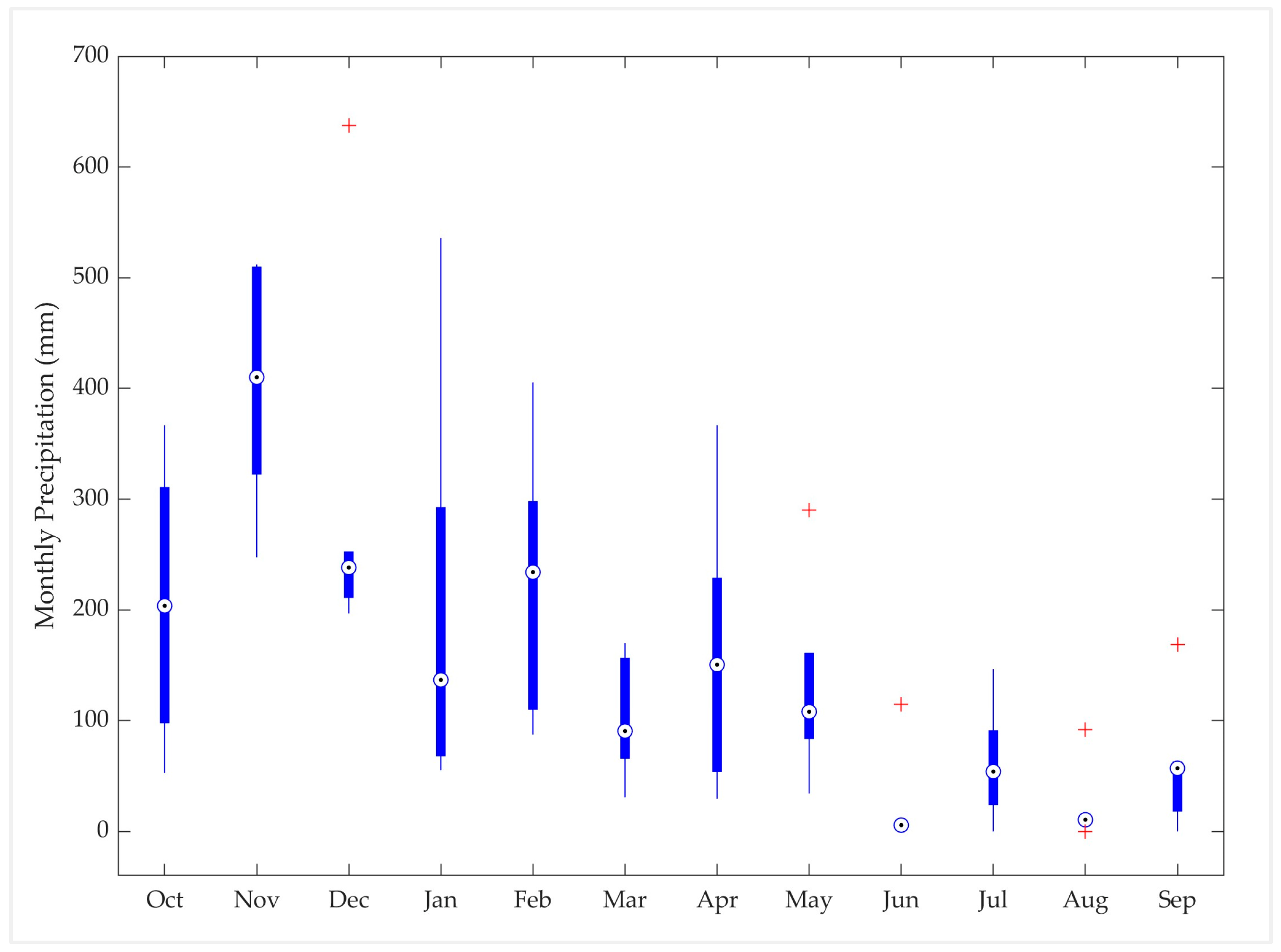
The Padiyathalawa sub-watershed is located in the intermediate zone of Sri Lanka [47]. It received an annual average precipitation of 2158 mm over the hydrological years between 1989 and 2020 [48]. Despite this relatively sizeable amount of annual precipitation, the downstream of the Padiyathalawa River Basin (i.e., middle and downstream areas of the Maduru Oya basin) is in the dry zone. There is also significant seasonal variation in rainfall, with seven months (March to September) contributing less than 30% of the annual total rainfall, which includes two months (June and August) experiencing almost no rainfall (Figure A1). Significant seasonal variations in precipitation cause stress on numerous sectors, including agriculture and the ecological environment. The First Inter-Monsoon (March to April) and the South-West Monsoon (May to September) seasons bring light rains, contributing only ~9% and ~20% to the annual precipitation. In contrast, the Second Inter-Monsoon (October to November) and the North-East Monsoon (December to February) seasons account for ~29% and ~42% of the annual rainfall, respectively. The yearly average temperature of this sub-watershed is ~24 °C [48].

2.2. Hydro-Meteorological Data Collection and Preprocessing

The observed data required for model setup, calibration, and validation (viz., rainfall, maximum and minimum temperature, and streamflow) was obtained from the Department of Irrigation and the Department of Meteorology in Sri Lanka (Table 1). Considering the data availability and spatial distribution of rain gauges, precipitation data from Welipitiya Coconut Estate was selected for the study. Moreover, the missing data percentages for the surrounding precipitation gauging stations are less than 10%, thus making them suitable for the closest station patching method [49] to estimate missing climatic data.
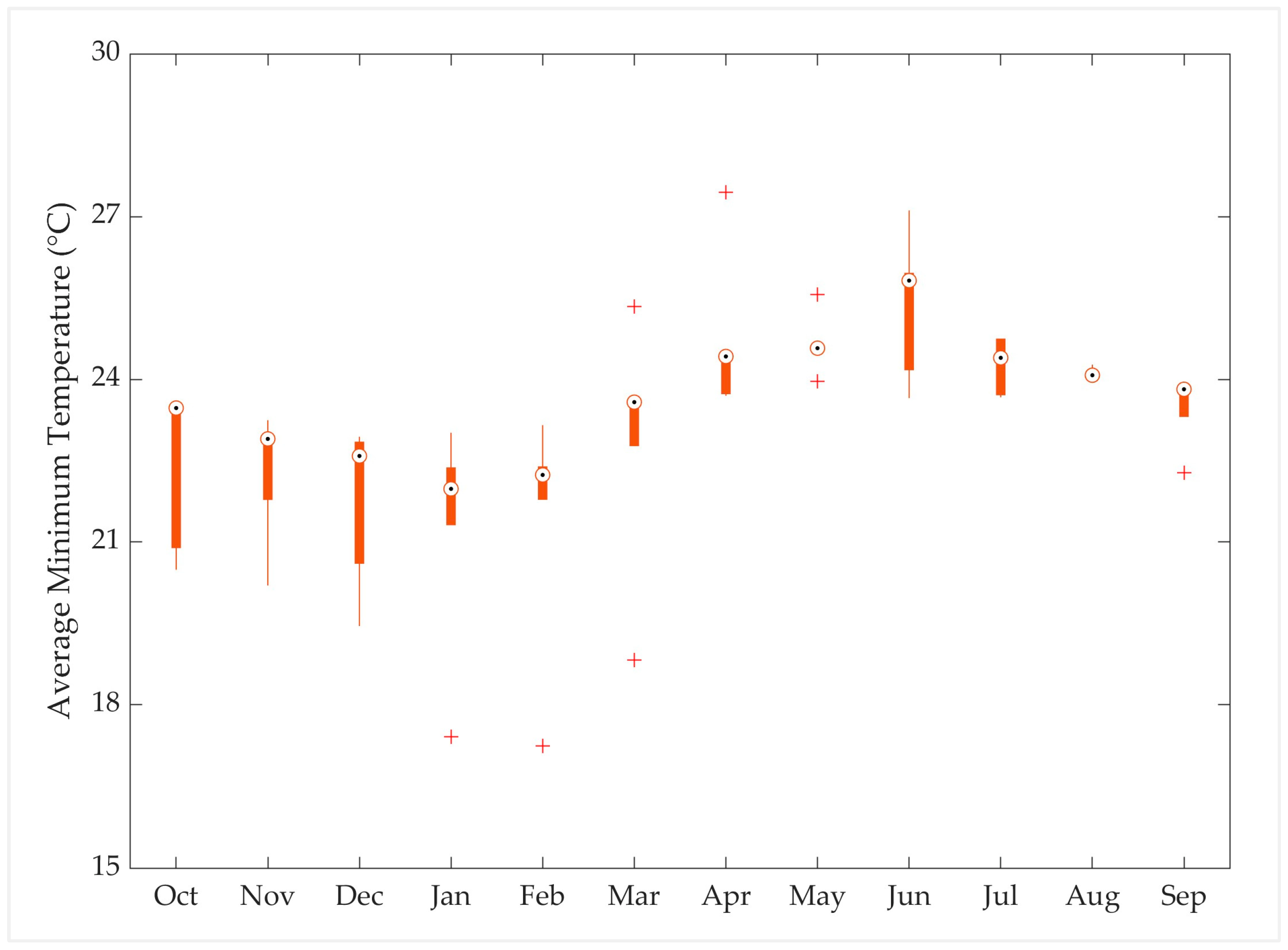
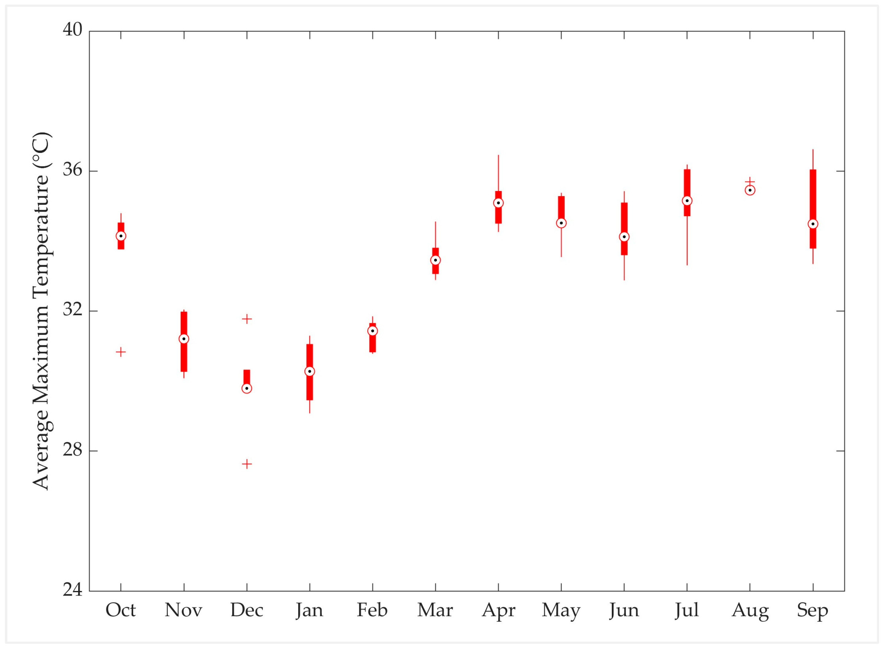
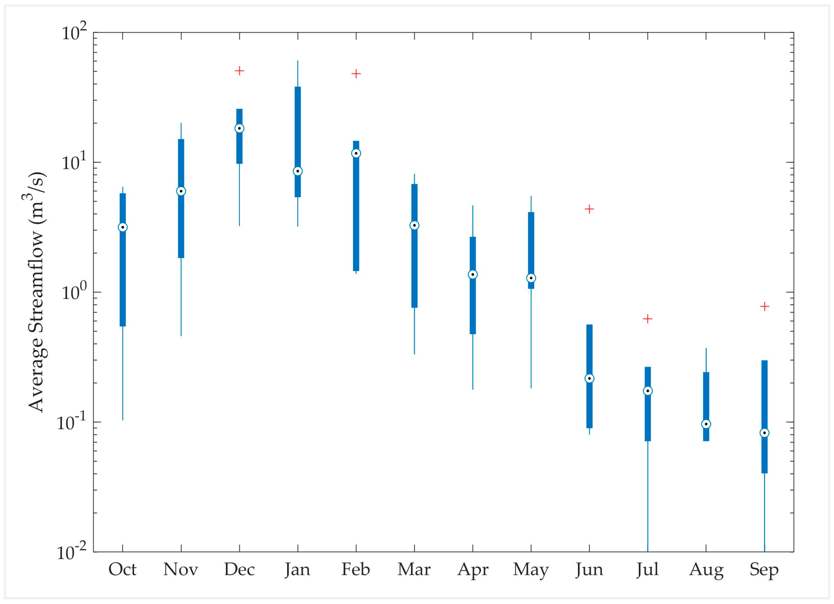
Similarly, temperature records at Maduru Oya station, with less than 10% of missing data, were gap-filled using the closest station patching method. There are no missing data in the Padiyathalawa streamflow measurements over the study period considered. Monthly variations of each hydro-meteorological data (viz., rainfall, minimum and maximum temperature, and streamflow) are shown in Appendix A Figure A1, Figure A2, Figure A3 and Figure A4.
Evaporation is one of the inputs required by the Tank Model. Since there are no in-situ measurements available, Hargreaves’ reference evapotranspiration model (1985) was used to calculate the reference evapotranspiration ( E T 0 ) at the Maduru Oya temperature gauge station (Figure 1). The limitations of a simple evapotranspiration model can be addressed by locally calibrating it using ET values obtained from a pan evaporation method [50]. Accordingly, the E T 0 values were calibrated with the in situ long-term average monthly pan evaporation (pan coefficient of 0.8) recorded at the Padiyathalawa gauging station [48]. The computation of Reference Evapotranspiration ( E T 0 ) is presented in Appendix B, and the calibration results are presented in Table A1.
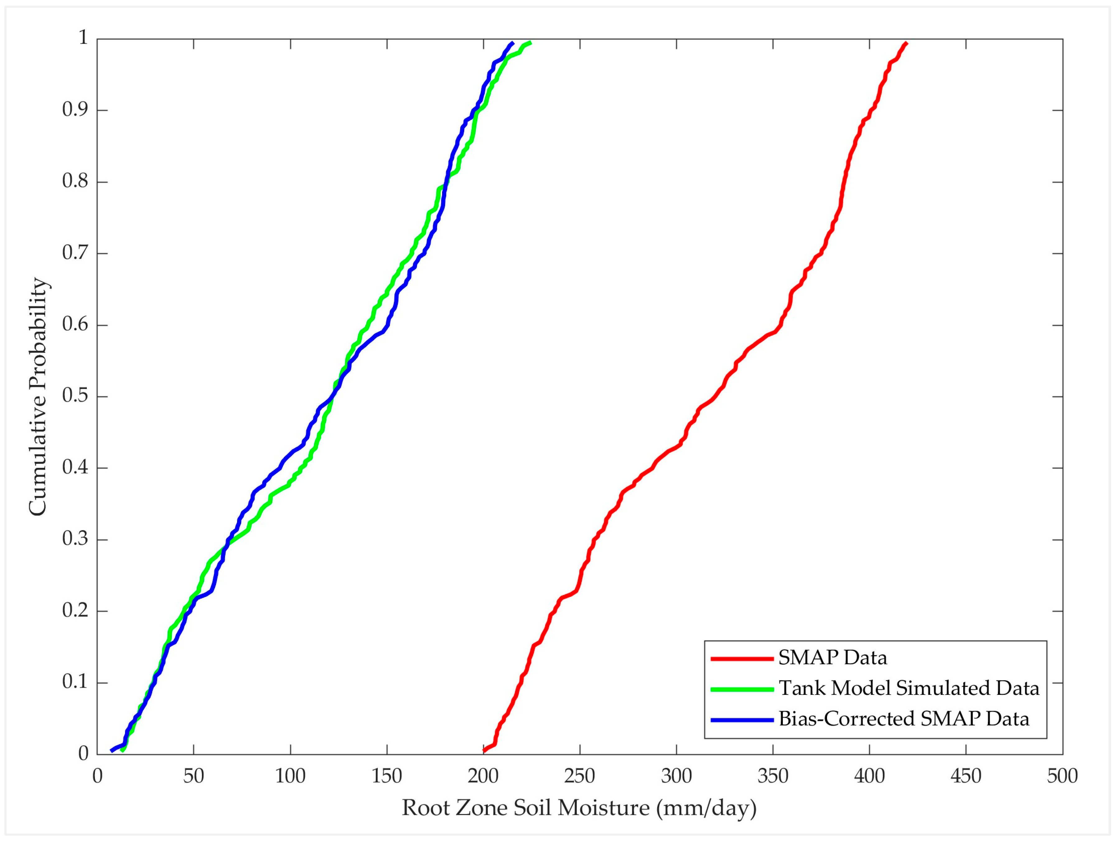
Remote-sensing-based soil moisture data (freely available at the National Snow and Ice Data Centre (NSIDC) [22]) and observed streamflow were used for the model calibration and validation. As the SMAP L4 retrievals are obtainable at the 3 h frequency for a particular location, it provides eight RZSM values for a given day. Preliminary data checking found no outliers in the dataset during the simulation period. Therefore, due to the minimal daily variations in these data, they were averaged using the simple arithmetic mean method to obtain daily values. The temporally aggregated data was then spatially aggregated using the Thiessen polygon method. It was noticed that the spatially and temporally aggregated RZSM data from SMAP comprise systematic biases. Even though the remote sensing data capture temporal variation, the Tank Model simulated soil moisture data show differences in its magnitude. Therefore, the spatially and temporally aggregated RZSM data was rescaled using the Cumulative Distribution Function (CDF) Matching method, and its outcome is shown in Figure A5.
Table 1. In situ and remote sensing data used for the analysis.
DatasetResolutionSource
Rainfall (six stations)DailyMeteorological Department, Sri Lanka
Temperature (two stations)DailyMeteorological Department, Sri Lanka
Streamflow (one station)DailyIrrigation Department, Sri Lanka
SMAP L4 root zone soil moisture3 hourly (9 km × 9 km)National Snow and Ice Data Centre Distributed Active Archive Center (NSIDC DAAC), USA
Digital Elevation Model30 m × 30 mShuttle Radar Topography Mission (SRTM)
Note: NSIDC data was obtained from https://nsidc.org/data/spl4smgp/versions/7 (accessed on 22 March 2024), and the Digital Elevation Model was obtained from the United States Geological Survey (USGS) Earth Explorer tool [51].

2.3. Hydrological Model Set-Up

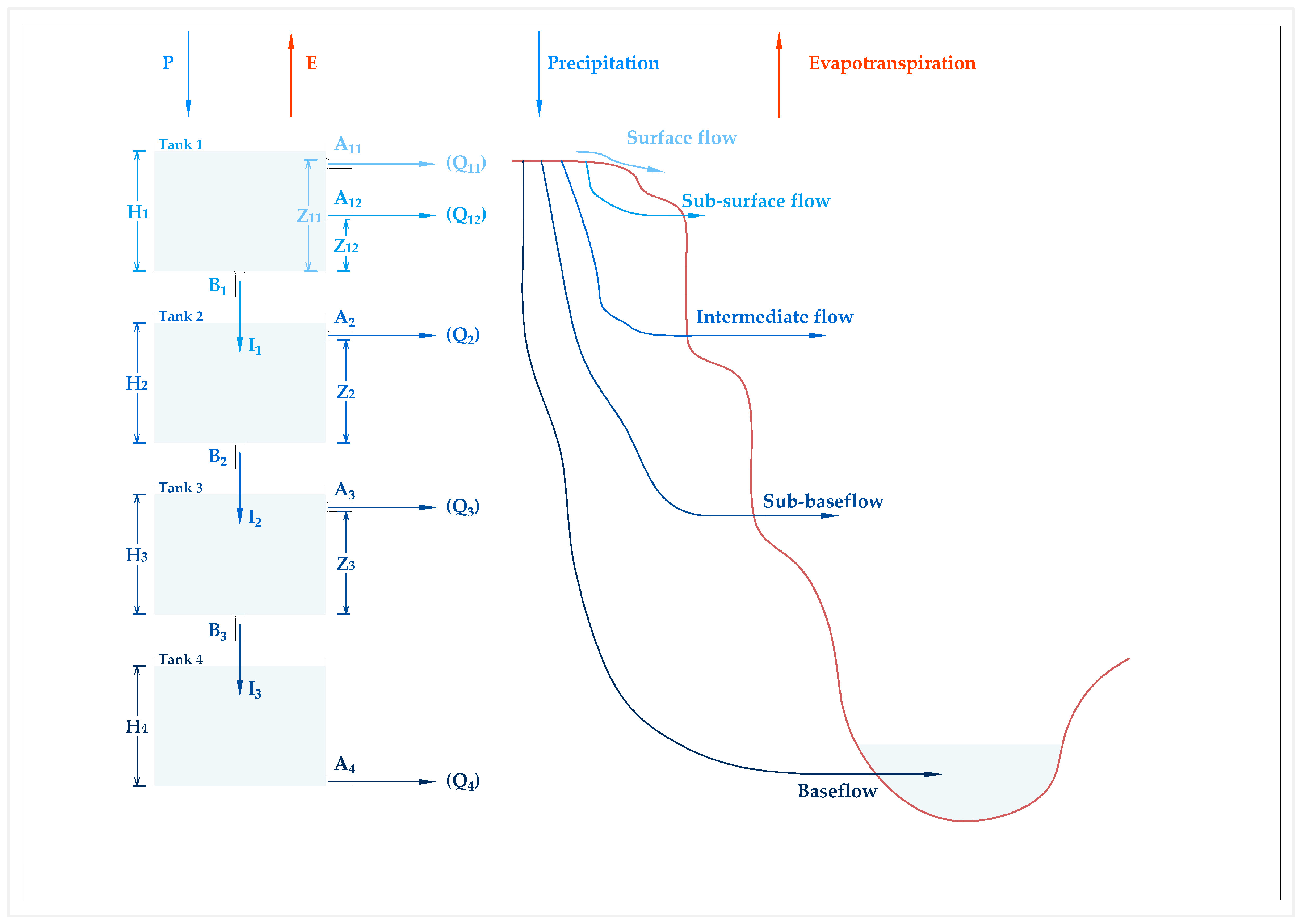
In this study, we selected the Tank Model, a lumped, non-linear, process-oriented Conceptual Rainfall-Runoff model developed by Sugawara [32]. Here, the series storage type is considered the best model among different Tank Models available (viz., exponential, parallel exponential, overflow, storage, and series storage) [32]. This model consists of several tanks vertically connected in series with bottom and side outlets to replicate the distinct watershed hydrological process (Figure 2). The series storage type Tank Model simulates the runoff as a function of the precipitation, evaporation, and antecedent soil moisture (or water storage in the soil), resulting in a non-linear deterministic model characteristic [52]. This model structure analyses the daily streamflow of an outlet consuming daily precipitation and evaporation inputs. The non-linear structure of the model accounts for initial abstraction [53]. It distributes the rainfall and assigns time lags to each component automatically. Further, it represents a reasonable physical representation corresponding to the groundwater structure. Despite its capability to describe the non-linear nature of surface runoff, it is challenging to determine the model parameters due to this non-linear behaviour [53]. Moreover, depending on the modelling objective and catchment characteristics, the series-storage type Tank Model has variations in the number of tanks and hydrological processes primarily considered. Among the numerous studies employing the Tank Model, Gunawardhana and Kazama [54] used it for a low-flow analysis under climate change conditions in the Tagliamento River in Italy. Yokoo et al. [55] regionalised the Tank Model parameters by relating them to catchment characteristics such as land use, topography, geology, and soil type. Goodazri et al. [56] investigated the effect of catchment scale on the Tank Model parameters, concluding that the model can be effectively applied even in larger river basins.
Many successful studies in which the Tank Model was used in different regions can be found in the literature (e.g., [53,57,58,59]). The Tank Model has been successfully employed in catchments as small as 15 km2 (Goodazri et al. [56]) and as large as 1935 km2 (Gunawardhana and Kazama [54]). Following Yokoo et al. [55] and Musiake and Wijesekera [60], the initial model parameters were estimated using catchment characteristics such as land use, topography, geology, and soil type. Model parameters were then further calibrated using observed river flow data to match the specific site conditions in the study area. When focusing on high flows, the parameters directly related to the surface runoff, such as A11, Z11, and A12, are identified as the most significant. On the other hand, low-flow characteristics are governed by the sub-baseflow and baseflow parameters, which respond to the river flow with a time lag. The variables of the hydrological model are determined by the site-specific characteristics. For example, in snow-fed river basins, a snow melt component governed by air temperature is added to the first tank [54]. Considering long-term simulations, evapotranspiration was included in the water balance computations of this study.
The model parameters required in the Tank Model can be clustered into two groups: (1) outlet coefficient (five parameters on the side walls, viz., A11, A12, A2, A3, and A4 and three parameters on the tank bottoms, viz., B1, B2, and B3) and (2) soil water storage coefficients (four runoff hole depths, viz., Z11, Z12, Z2, and Z3) [52,57,59,61]. The output from the side outlet of the top tank (i.e., Tank 1) is surface runoff, and the output from the second tank is intermediate runoff. The outputs from the third and fourth tanks are considered to account for low-flow situations via the sub-base flow and baseflow, respectively (Figure 2). Mathematical interpretations of the Tank Model are illustrated in the following Equations (1)–(4),
Q x , n = A x × H x , n Z x ; H x , n > Z x 0 ;     H x , n Z x
I x , n = B x × H x , n
H x , n = H x , n 1 Q x , n × t I x , n × t + P n E n × t ; x = 1 H x , n 1 Q x , n × t I x , n × t + I x 1 , n × t ; x 1
Q T , n = x = 1 4 Q x , n
where x is the tank count, starting from the top; n is the count of days since the simulation starts (days); t is the time interval (days); A x is the runoff coefficient of the x t h tank (1/day); B x is the infiltration coefficient of the x t h tank (1/day); H x is the water depth in the x t h tank (mm); Z x is the runoff hole depth of the x t h tank (mm); Q x is the contribution to the streamflow from the x t h tank (mm/day); I x is the infiltration from the x t h tank (mm/day); P is precipitation (mm/day); E is evapotranspiration (mm/day), and Q T is the total streamflow (mm/day).
As this study focuses on a dry watershed with seasonal variations in precipitation, the Tank Model developed for humid regions is applied [53]. The typical hydrological model parameters are directly measured physical or calibrated process parameters. However, the Tank Model is designed for the calibrated process parameters [62]. The Tank Model parameters can be calibrated either manually (using a trial-and-error process) [63] or automatically by the use of computer-aided complex mathematical formulations [64]. Although automatic calibration improves the efficiency, stability, and consistency of the model performance [63,65], its major drawback is the determination of initial parameters that govern the computer algorithm to achieve the optimal parameters [52]. Generally, determining the realistic initial value becomes challenging because it requires experience and user knowledge of the model and the study area [52]. However, the effectiveness of the Tank Model depends on the degree of calibration [45], which can be improved by using automatic calibration in conjunction with manual calibration [57,65]. Initial model parameters used in this study (Table 2) were assigned based on the Tank Model parameters optimised for the Mahaweli River Basin in Sri Lanka [60].
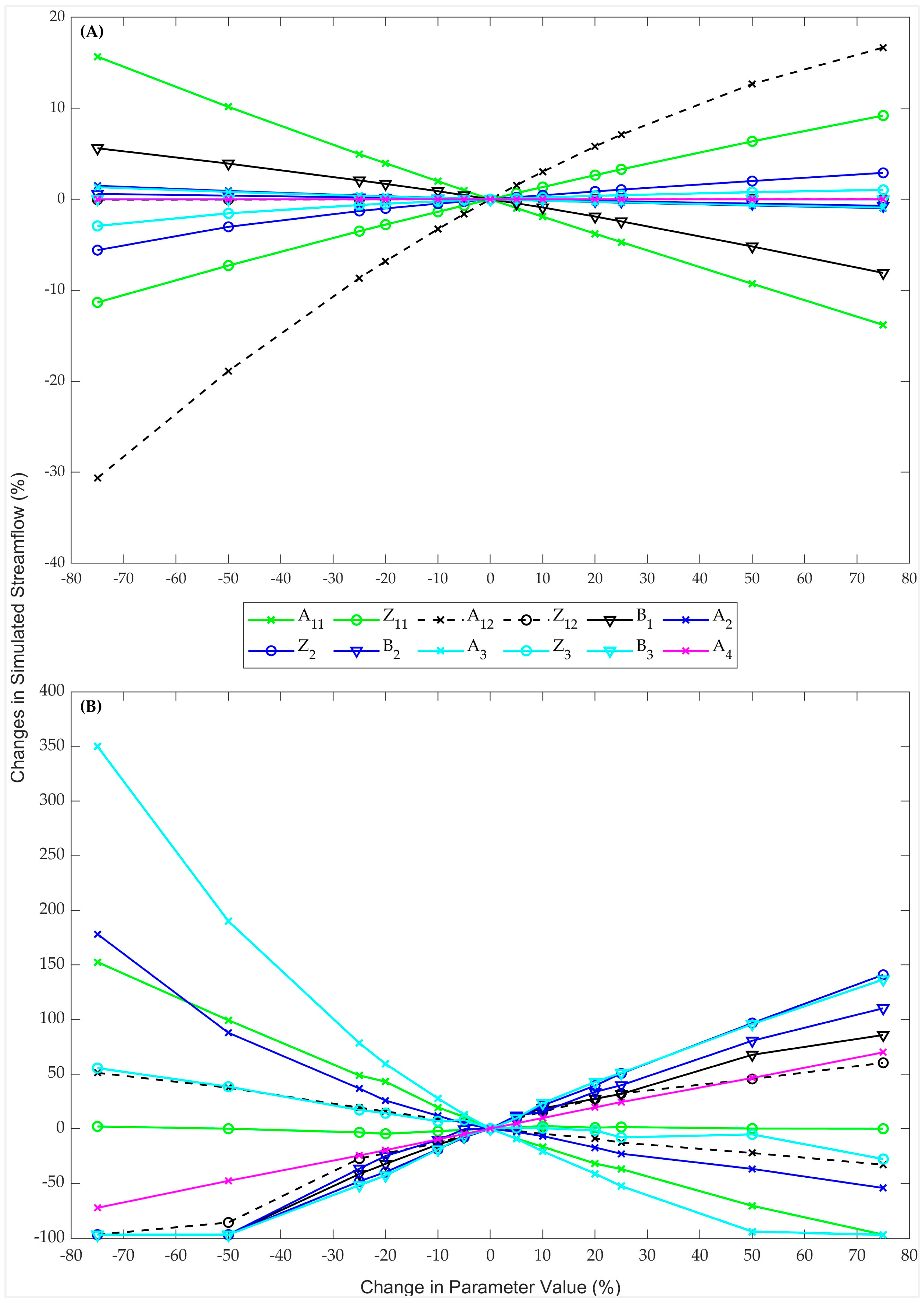
A sensitivity analysis was conducted to identify the parameter sensitivity to the peak and low flow simulation, in which the adopted initial values varied between −75% and 75% to evaluate their contributions to the observed flow between October 2010 and September 2015 (Figure 3). A one-year warm-up period was considered before two datasets were considered during the study to initialise the water storage in each tank under three cycles, assuming all tanks were empty during the initial round.

2.4. Objective Function for Model Optimisation

The performance of hydrological model simulations can be evaluated by numerous statistical indices, including the Nash–Sutcliffe efficiency (NSE), Nash and Sutcliffe, Kling–Gupta efficiency (KGE) [66], and Root Mean Square Error (RMSE). The Nash–Sutcliffe Efficiency (NSE) tends to be overly sensitive to high-flow values. Moreover, its use of the observed mean as a baseline can result in overestimating model performance for highly seasonal variables, such as river flow in dry basins [67]. One of the major limitations of the RMSE is that it is more influenced by a few large errors in the simulation, which may not provide a balanced view of model performance [68]. Both NSE and RMSE provide a single aggregated measure of error, which can mask the underlying reasons for poor model performance.
The KGE was explicitly designed to balance the sensitivity to bias and variability. It decomposes the error into three components: correlation (r), variability (α), and bias (β), allowing an understanding of different aspects of model performance, indicating temporal pattern, mean difference, and dispersion difference between observed and simulated data, respectively. Therefore, the KGE ensures a more balanced evaluation of the model performance across different flow conditions [69].
The Kling–Gupta Efficiency is defined as the Euclidean Distance (ED) to the point measured from the ideal point (5). The KGE values can vary between and 1.0, with the latter indicating a perfect model accuracy [66].
K G E = 1 E D = 1 r 1 2 + α 1 2 + β 1 2
Here, r is the linear correlation coefficient between the observed and simulated data (6), α is the relative variability between observed and simulated data (7), and β denotes the bias (8);
r = i = 1 n O i O ¯ P i P ¯ i = 1 n O i O ¯ 2 i = 1 n P i P ¯ 2
α = σ S σ O
β = μ S μ O
where μ S and μ O are the mean values of simulated and observed data, respectively, σ S and σ S are the standard deviations of simulated and observed data, respectively.

2.5. Model Calibration and Optimisation

The model calibration procedure involves two steps, single- and multi-variable, undertaken between August 2011 and September 2012. The calibrated model was validated with data between September 2015 and April 2016.

2.5.1. Single-Variable Calibration

The single-objective calibration approach was employed to optimise the model with observed daily streamflow data utilising KGE ( K G E Q ) for the calibration period. The model was calibrated based on the initial parameters developed for the upper Peradeniya catchment (Table 2) [60]. The results were validated using the observed data between September 2015 and April 2016.

2.5.2. Multi-Variable Calibration

A weighted objective function (9) was used under 11 calibration schemes, where the weighted factor (ϑ) varies between 0 and 1.0, with 0.1 increments. This calibration was undertaken between September 2015 and April 2016, constrained by the availability of calibration variables (viz., streamflow and remote-sensing-based soil moisture).
K G E w = 1 ϑ K G E Q + ϑ . K G E S M
Microsoft Excel’s Solver includes one linear and two non-linear solver functions (Generalized Reduced Gradient (GRG) and evolutionary solver), and the GRG solver has been widely used in hydrological studies. Given the non-linear nature of the hydrological processes involved in basin water balance, this study employs the GRG method to estimate the parameters of the Tank Model, focused on optimising the weighted KGE function (9). All the twelve model parameters (Table A2) were set as changing variables, constrained by their respective upper limits. For multi-variable optimisation, the GRG Non-linear method [70] was selected while assuming the optimisation problem to be smooth and non-linear, which is an assumption involved in other studies (e.g., [71,72,73]).
Here, the Multi Start option was enabled for a population size of 20, which commences the calibration with unique starting points per each population class. Since the random seed was set to zero, the program selects each starting point randomly, preserving the diversity of solutions. The chosen population size yielded a satisfactory convergence (tolerance margin of 0.0001) through single-objective optimisation, swiftly converging the multi-variable optimisation to an adequate level. Furthermore, two commonly used tests (viz., t-test [74] and Wilcoxon signed-rank test [75]) were employed to identify the statistical significance of the model performance improvement in two calibration schemes.

3. Results

The content of this section is structured into three sub-sections. The first sub-section presents the findings of the parameter sensitivity analysis. The second and third sub-sections present performances under single- and multi-variable calibrations.

3.1. Parameter Sensitivity

The results of the sensitivity analysis are presented in Figure 3. Here, the model parameters can be categorised based on their sensitivity levels towards peak and low flows (highly sensitive, moderately sensitive, and less sensitive). The highest flow rate during the simulation period was used as the reference value for peak flow analysis, while the 25th percentile of the flow rate was used for low-flow analysis. A higher percentile was selected for the low-flow sensitivity analysis due to the large number of zero flow rates (no flows) occurring during the dry period. Parameters of the first tank (A11, A12, Z11, Z12, and B1), which are related to infiltration and surface, sub-surface, and intermediate flow, as well as the runoff coefficient of the second tank (A2), were found to have higher sensitivity towards high flows. In contrast, parameters in other tanks (Z2, B2, Z3, A3, B3, and A4) were found to be trivial for producing high flow rates. These less-sensitive parameters represent the intermediate flow, infiltration, base flow, and sub-base flow of different tanks. Baseflow and sub-baseflow parameters were found to be more sensitive for low flows. For example, increases in parameters Z2 and B3 positively affect low flows, while decreases in parameters A11, A2, and A3 also positively affect low flows. This phenomenon can be explained by the fact that as surface runoff decreases due to lower corresponding parameters, infiltration and percolation increase, enhancing low flows.

3.2. Model Performances in Single-Variable Calibration

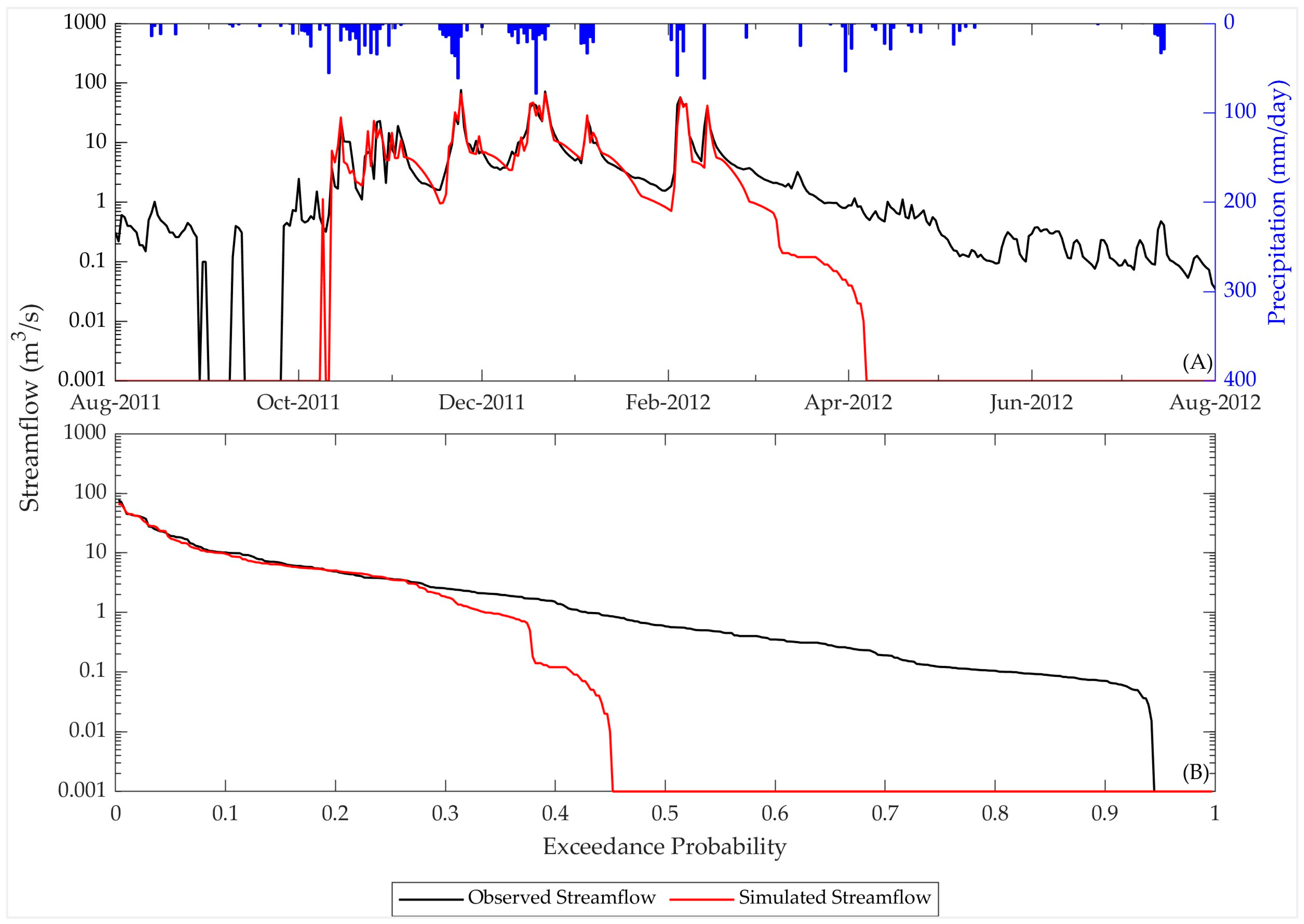
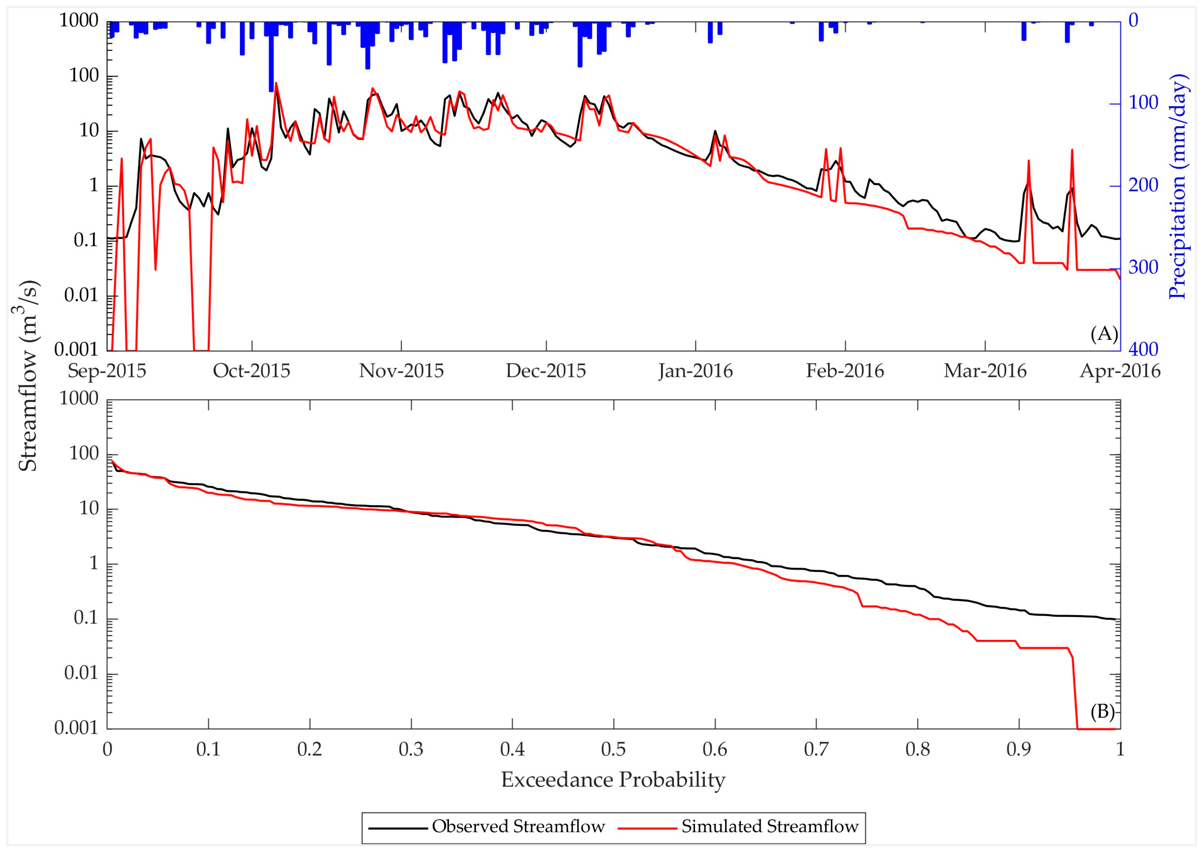
The single-variable calibration using observed streamflow data provides satisfactory streamflow simulations in both calibration (Figure 4) and validation (Figure 5), with respective K G E Q values of 0.87 and 0.85. However, the hydrographs (Figure 4A) and the Flow Duration Curves (FDCs) (Figure 4B) in calibration show marginal underestimations in the peak-flow and low-flow simulations.

3.3. Model Performances in Multi-Variable Calibration

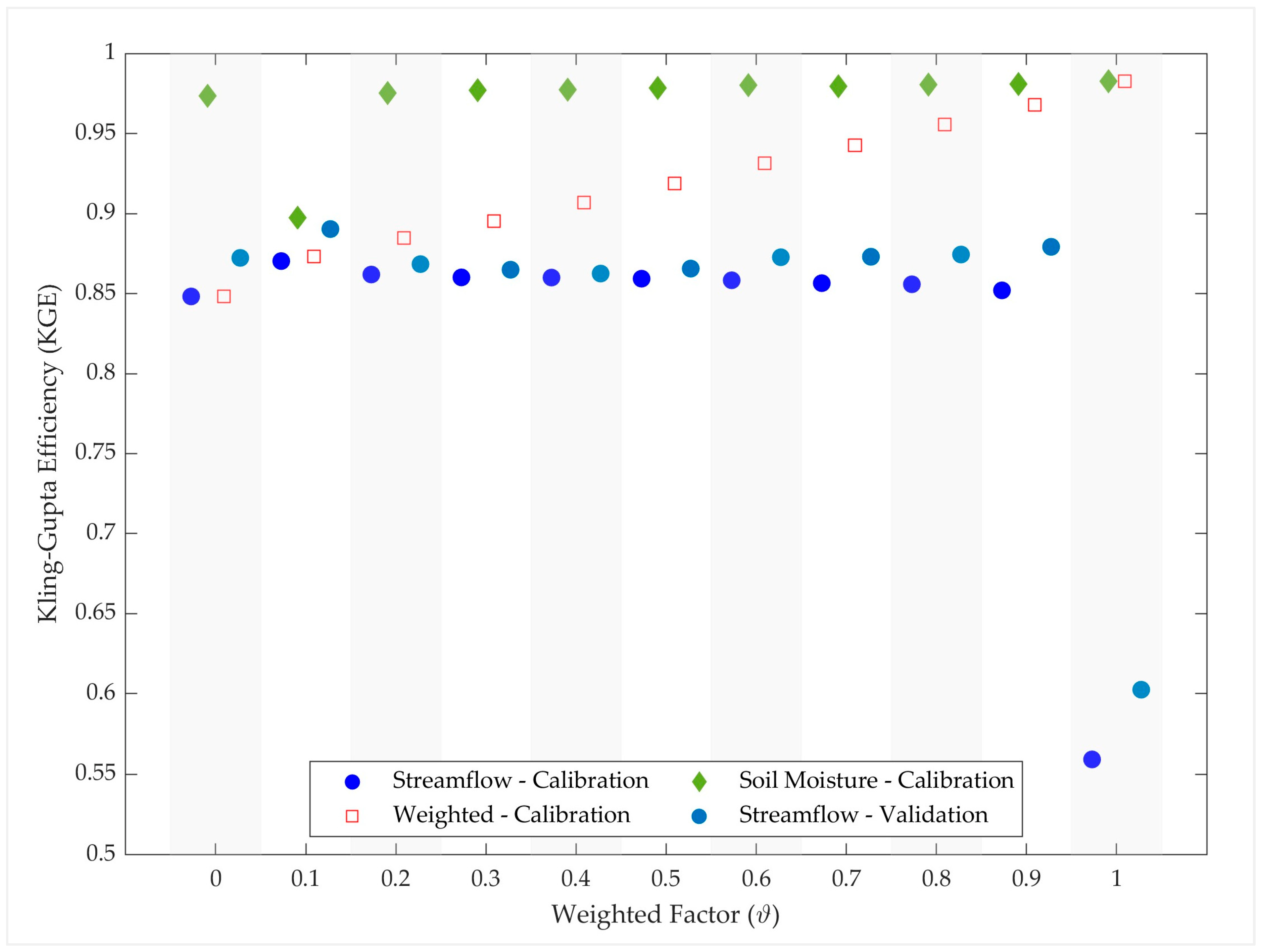
The multi-variable calibration performances in terms of KGE are presented in Figure 6. The two extreme calibration schemes, viz., ϑ = 0 and ϑ = 1.0 represent the single variable optimisations with streamflow and root zone soil moisture, respectively. Except for the ϑ = 1 calibration scheme (i.e., single variable optimisation with soil moisture), model performances in streamflow and soil moisture show satisfactory results under all other schemes tested in this study. The calibration scheme of ϑ = 1 shows that the single objective optimisation with soil moisture fails to produce accurate streamflow simulations. Figure 6 clearly shows that the weighted KGE ( K G E W , (9)) increases from ϑ = 0.2 scheme onwards, causing slight increases in K G E S M and slight decreases in K G E Q with a drastic decrease at ϑ = 1 scheme. Therefore, it is evident that, from a multi-variable perspective, higher weightage on root zone soil moisture can enhance the overall model performance in terms of K G E W .
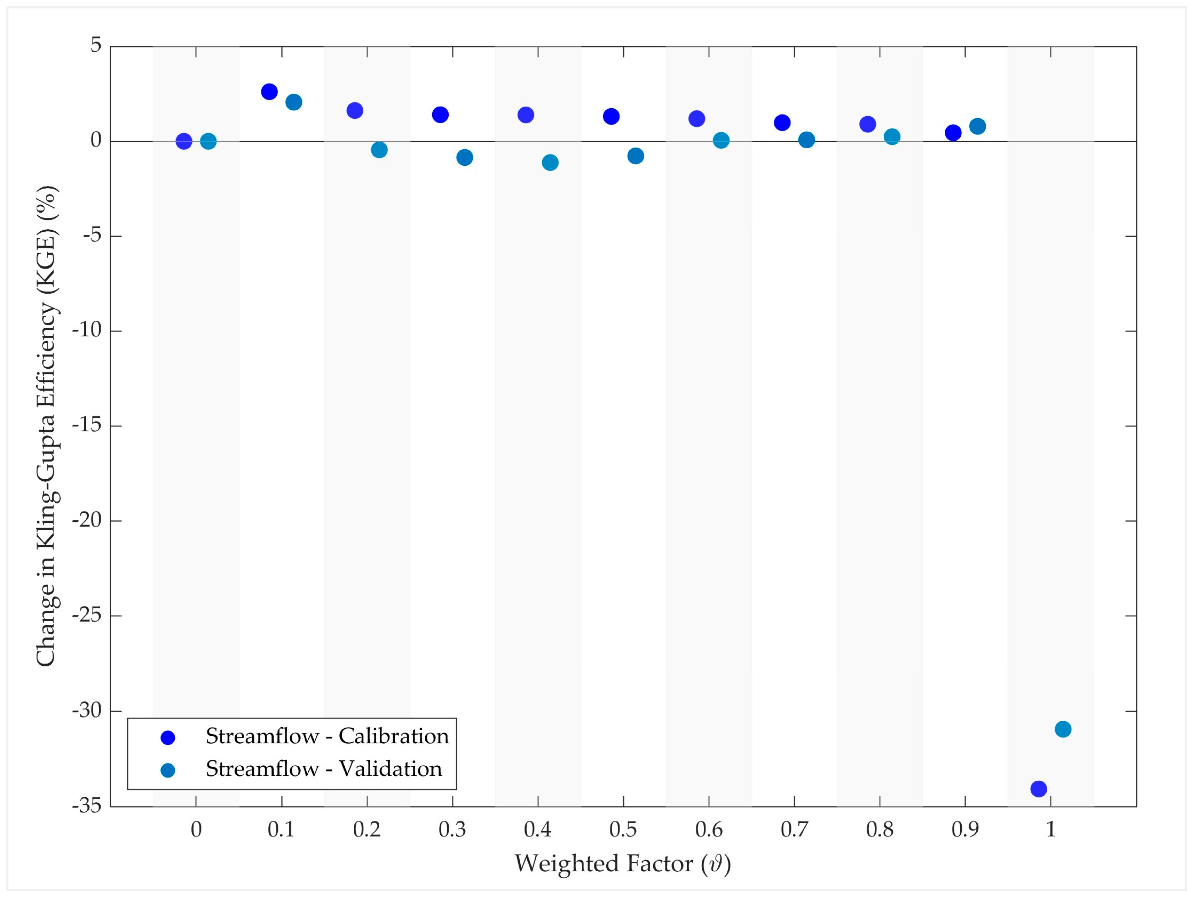
Figure 7 illustrates the percentage change in K G E Q resulting from multi-variable calibration compared to single-variable across all calibration schemes. Among the accuracy-increased calibration schemes (ϑ values of 0.1, 0.8, and 0.9), the ϑ = 0.1 scheme yields the most accurate streamflow simulation, with a K G E Q of 0.87 and 0.89 in calibration and validation, respectively. However, despite offering a better simulation with K G E S M of 0.90, it exhibits lower accuracy in soil moisture simulation than other schemes (Figure 6). Regarding the calibration schemes, the best RZSM simulation is observed with the ϑ = 0.9 scheme. Nonetheless, since this study’s primary focus is on accurate streamflow simulation in the catchment, the calibration scheme of ϑ = 0.1 is deemed more suitable as it provides the highest accuracy in streamflow simulation, even during the validation period with a K G E Q of 0.89.
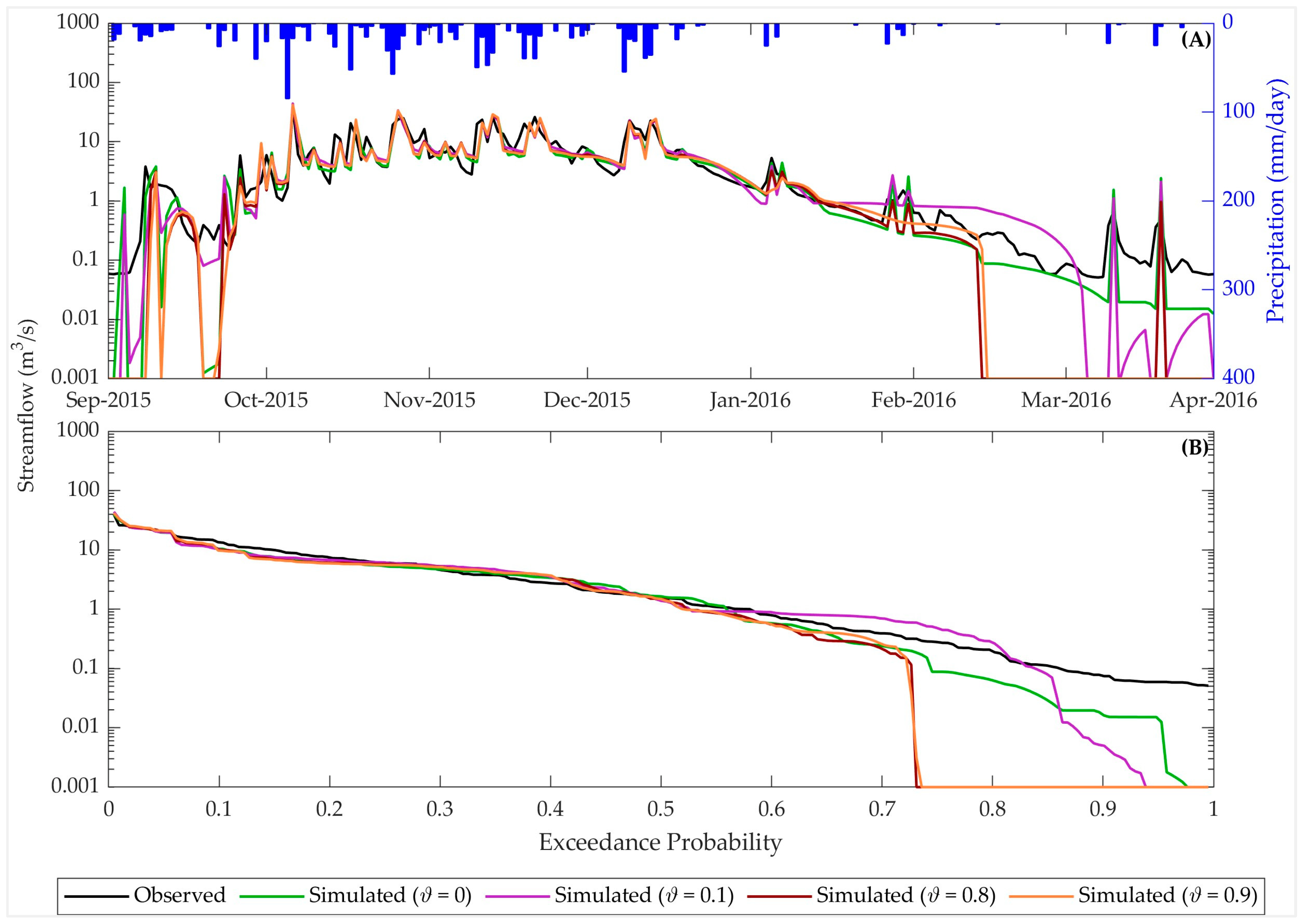
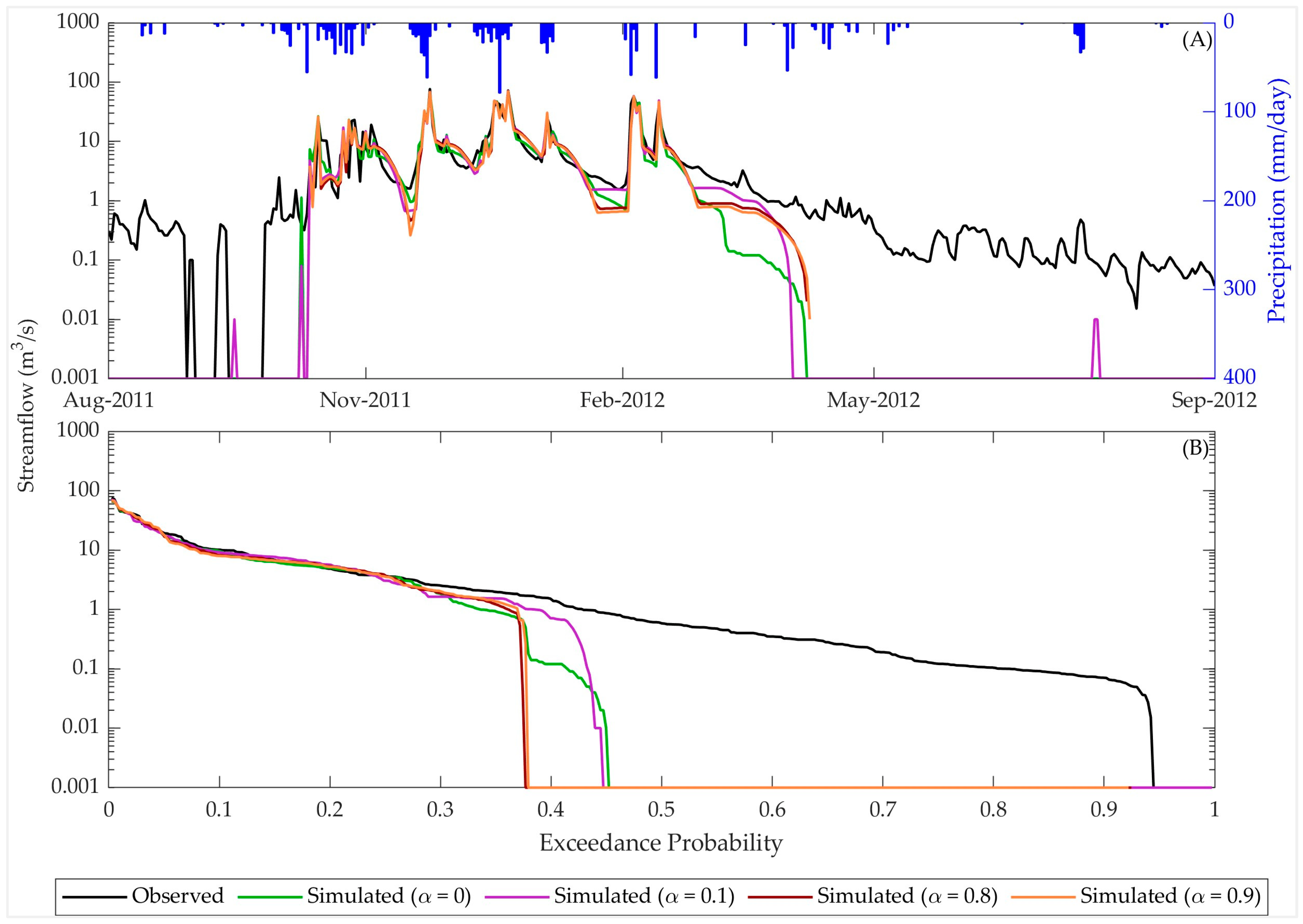
The simulated streamflow and FDCs for the better-performing (i.e., accuracy-increased) calibration schemes with weighted factor (ϑ) of 0.1, 0.8, and 0.9 are illustrated in Figure 8. It shows that the calibration scheme of ϑ = 0.1 underestimates the peak and low flows. However, compared to the single-variable calibration (i.e., ϑ = 0), the ϑ = 0.1 calibration scheme provides better peak and lower flow estimations. The other two calibration schemes (i.e., ϑ = 0.8 and ϑ = 0.9) considerably underestimate the low flows (Figure 8).
The streamflow simulations and FDCs of the better-performing schemes during the validation period (between August 2011 and September 2012) are shown in Figure 9. It shows that, even for low flow conditions, the calibration scheme ϑ = 0.1 provides better estimations than the single-variable calibration (i.e., ϑ = 0). As identified in the calibration, the calibration schemes ϑ = 0.8 and ϑ = 0.9 cannot simulate low flow conditions satisfactorily.
The soil moisture variation under accuracy-increased calibration schemes of ϑ = 0.1, 0.8, and 0.9 are shown in Figure 10. As discussed earlier, the calibration scheme ϑ = 0.1 shows the minimum agreement between the observed and simulated soil moisture. The calibration scheme with a 0.9 weighted factor (ϑ) shows better agreement in observed and simulated soil moisture content.

4. Discussion

Our results show increased model performance (i.e., better KGE values) under multi-variable calibration than a single variable. As an example, calibration schemes with weighted factors (ϑ) of 0.1, 0.8, and 0.9 show more accurate streamflow simulations than the single-variable calibration, even in the validation period. These better performances can be attributed to the behaviour of different calibration parameters. For example, A11 and A12 coefficients, which enhance the surface and sub-surface flows, are higher for the ϑ = 0.1 than ϑ =0 (viz., single-variable calibration with streamflow), resulting in more accurate simulations of the peak flows. Also, higher B1, B2, and B3 values enhance the water percolation up to the groundwater table, and greater A3 and A4 coefficients increase the base-flow contribution. Even though overall model performances ( K G E Q ) are higher under ϑ = 0.8 and 0.9 calibration schemes, those schemes significantly underestimate the low flows due to considerably low A3 and A4 coefficients (Table A2) (compared to the same in calibration under ϑ = 0.1). Previous studies (e.g., Xiong and Zeng [21]) have concluded that using multiple variables enhances the reliability of optimised parameters, even if the overall model performance is less than that of single-variable optimisation. The KGE used in this study assesses different aspects of model performance, including correlation, variability, and bias. We evaluated the increases in model performance using the paired two-sample t-test and Wilcoxon signed-rank test, in which 8.5% and 24.7% statistical improvements are observed with the respective tests.
The literature shows that the multi-variable calibration using in situ streamflow and remote sensing-based soil moisture data can marginally reduce the streamflow simulation during the calibration compared with single-variable calibration with streamflow [21,76]. Further, Xiong and Zeng [21] utilised SMAP Level 3 surface soil moisture retrievals converted to the Soil Wetness Index of the root zone, potentially resulting in a less accurate representation of catchment soil–water conditions compared to the direct RZSM retrievals from SMAP L4 used in this study. The conclusions drawn by Gunasekara et al. [76] are controversial, even though their research utilised the lumped hydrological model (ABCD Model, ref. [29]) and SMAP L4 RZSM data in a daily time resolution similar to this study. However, Gunasekara et al.’s study [76] differs from ours in that it features a significant water body within the study area, which poses challenges to the applicability of a lumped hydrological model.
Simply put, the Tank Model used in this study successfully conceptualised the hydrology of the study area. Eini et al. [77] also used streamflow and Climate Change Initiative Soil Moisture dataset in the multi-variable calibration of the Soil and Water Assessment Tool+ (SWAT+, ref. [78]) in a sizeable transboundary basin (viz., Odra River Basin) in Central Europe. They concluded that the multi-objective calibration could substantially improve the accuracy of the simulations with an average KGE of 0.67 compared to an average KGE of 0.60 in single-variable calibration. A study by Loizu et al. [24] used Advanced SCATterometer Surface Soil Moisture data to improve the streamflow simulations in Mediterranean catchments through different data assimilation techniques. Therefore, careful evaluation of potential remote sensing soil moisture products is essential in hydrological model calibration to improve the performance of streamflow and other water balance components simulations in varied regions.
Besides soil moisture data, other remote-sensing-based variables are used in multi-variable calibration to enhance the hydrological model performances, particularly in data-scarce regions. For example, Sirisena et al. [8] used remote sensing-based evapotranspiration data from Global Land Evaporation: the Amsterdam Model (GLEAM ET) along with streamflow in the Chindwin River Basin in Myanmar, where in situ measurements are sparse. They also suggested that multi-variable calibration offers good performance in streamflow while maintaining reasonable performances when simulating the catchment’s evapotranspiration. Furthermore, Rientjes et al. [79] indicated that the water balance of the Karkheh River Basin, Iran is best reproduced by streamflow and satellite-based evapotranspiration data used during the hydrological model calibration. Therefore, it is evident that the potential use of different satellite-based products as alternative sources in hydrological model calibration may return dividends over traditional calibration, particularly in data-poor regions with limited streamflow records.

5. Conclusions

This study focused on assessing the significance of multi-variable calibration in hydrological simulations in a data-scarce dry river basin by utilising in situ streamflow and remote sensing-based soil moisture data (viz., SMAP L4) in single- and multi-variable calibration schemes using a lumped hydrological mode (viz., the Tank Model). The proposed method was piloted at the Padiyathalawa sub-basin of Madura Oya Basin, Sri Lanka. For the multi-objective calibration, a series of weighted factors (ϑ), between 0 and 1.0 (at 0.1 intervals), were used, and the performances were assessed using the Kling–Gupta Efficiency (KGE). This study is one of the few studies conducted in the region to investigate the possibility of improving hydrological model performances using Soil Moisture Active Passive Level 4 (SMAP L4) under different calibration schemes (i.e., single- and multi-variable). Furthermore, the lumped Tank Model can successfully represent the catchment dynamics, particularly in small catchments such as the Padiyathalawa sub-watershed.
With single-variable calibration (i.e., streamflow only), both calibration and validation showed higher model efficiency criteria (KGE > 0.83), even though it slightly underestimates the peak flows while considerably underestimating the low flows. Three multi-variable calibration schemes with 0.1, 0.8, and 0.9 weighted factors (ϑ) showed better streamflow simulations ( K G E Q > 0.85 for both calibration and validation) than the single-variable calibration. Therefore, incorporating root zone soil moisture into the weighted multi-objective function improves the overall performance of the Tank Model. However, the calibration scheme of 0.1 weighted factor (ϑ) is more capable of simulating the streamflow dynamics, particularly the low flows, than the other two better-performing calibration schemes (ϑ of 0.8 and 0.9). Therefore, the calibration scheme with a 0.1 weighted factor (ϑ) is more suitable for conceptualising the catchment dynamics at the Padiyathalawa sub-watershed, underscoring the effect of the minimal contribution from root zone soil moisture translating into significantly improved streamflow simulations in terms of accuracy and reliability.
It is important to note that this study’s calibration and validation periods were intentionally kept short due to significant inconsistencies in the hydro-meteorological data. As the calibration and validation periods within this limited dataset may not accurately represent the long-term catchment flow dynamics, it is essential to validate these results with long-term data better to assess the robustness of the proposed modelling technique. Also, exploring alternative multi-variable optimisation techniques, such as genetic algorithms, is recommended. Furthermore, it is worth exploring the suitability of other remote-sensing-based soil moisture products and hydrological variables like evapotranspiration in enhancing the hydrological model’s performance within the study area.

Author Contributions

Conceptualisation, K.P., L.G., J.B. and J.S.; methodology, L.G. and K.P.; software, K.P.; validation, K.P. and L.G.; formal analysis, K.P.; investigation, K.P.; resources, L.R.; data curation, K.P.; writing—original draft preparation, K.P.; writing—review and editing, L.G., J.B., J.S. and L.R.; visualisation, K.P. and J.B.; supervision, L.G.; project administration, L.G.; All authors have read and agreed to the published version of the manuscript.

Funding

This research received no external funding.

Data Availability Statement

The raw data supporting the conclusions of this article will be made available by the authors, without undue reservation, to any qualified researcher. All data requests are encouraged to CC [email protected] for swift processing, monitoring, and administrative purposes.

Acknowledgments

This study could not have been possible without the support from the Irrigation Department and the Department of Meteorology, Sri Lanka, by freely issuing the data needed in the research, for which the authors are very grateful. The authors are thankful for the generous support extended by the UNESCO-Madanjeeth Singh Centre for South Asia Water Management (UMCSAWM), University of Moratuwa.

Conflicts of Interest

The authors declare no conflicts of interest.

Appendix A

Figure A1. Monthly precipitation at Welipitiya Coconut Estate gauging station between October 2010 and September 2016. The boxes are limited to the 25th and 75th percentiles, and the horizontal line shows the median (i.e., 50th percentile) value of the monthly data sets. Whiskers are extended to 1.5 times inter-quartile range to the top and bottom of the boxes.
Hydrology 11 00116 g0a1
Figure A2. Average minimum temperature measured at Maduru Oya gauging station between October 2010 and September 2016. The boxes are limited to the 25th and 75th percentiles, and the horizontal line shows the median (i.e., 50th percentile) value of the monthly data sets. Whiskers are extended to 1.5 times inter-quartile range to the top and bottom of the boxes.
Hydrology 11 00116 g0a2
Figure A3. Average maximum temperature measured at Maduru Oya gauging station between October 2010 and September 2016. The boxes are limited to the 25th and 75th percentiles, and the horizontal line shows the median (i.e., 50th percentile) value of the monthly data sets. Whiskers are extended to 1.5 times inter-quartile range to the top and bottom of the boxes.
Hydrology 11 00116 g0a3
Figure A4. Monthly averaged streamflow measured at Padiyathalawa gauging station between October 2010 and September 2016. The boxes are limited to the 25th and 75th percentiles, and the horizontal line shows the median (i.e., 50th percentile) value of the monthly data sets. Whiskers are extended to 1.5 times inter-quartile range to the top and bottom of the boxes.
Hydrology 11 00116 g0a4

Appendix B

Hargreaves and Samini model (1985) for Reference Evapotranspiration ( E T 0 )
E T 0 = 0.0023 R a T m a x + T m i n 2 + 17.8 T m a x T m i n
where E T 0 is the Reference Evapotranspiration (mm), T m i n and T m a x are the daily minimum and maximum air temperatures (°C), respectively.
R a is Extra-terrestrial Solar Radiation (MJm−2day−1), estimated according to Allen et al. [80].
R a = 24 ( 60 ) π G s c d r [ ω s sin Φ sin δ + cos Φ cos δ sin ω s ]
where G s c is Solar Constant (0.0820 MJm−2min−1) and Φ is Latitude (rad).
Inverse Relative Distance Earth–Sun ( d r ) is computed according to (A3).
d r = 1 + 0.033 cos 2 π 365 J
Solar Declination ( δ in rad) is computed as (A4),
δ = 0.409 sin 2 π 365 J 1.39
where J is the number assigned to the date of each year.
Sunset Hour Angle ( ω s in rad) is given by (A5).
ω s = arccos tan Φ tan δ
Table A1. Hargreaves evapotranspiration model calibration using the Pan evaporation method.
MonthObserved Pan Evaporation (mm)Simulated ET0 (mm)Evaporation Coefficient
October1171450.65
November871300.54
December721360.42
January791430.44
February901340.54
March1261580.64
April1241630.61
May1331650.65
June1531560.78
July1651620.82
August1611530.84
September1451450.8
Figure A5. Cumulative Distribution Function (CDF) Matching method-based rescaling of spatially and temporally aggregated Root Zone Soil Moisture data.
Hydrology 11 00116 g0a5

Appendix C

Table A2. Optimised model parameters and model performances under multi-variable calibration with weighted factor (ϑ).
Weighted Factor (ϑ)
00.10.20.30.40.50.60.70.80.91.0
K G E Q 0.850.870.860.860.860.860.860.860.860.850.56
K G E S M 0.970.900.980.980.980.980.980.980.980.980.98
K G E W 0.850.870.880.900.910.920.930.940.960.970.98
B 1 0.250.370.330.340.350.310.300.310.290.260.14
A 11 0.340.390.450.420.410.400.430.410.460.530.01
A 12 0.190.210.130.160.180.160.130.160.080.001.00
Z 11 14.9916.6221.7419.1318.3419.3119.9518.9820.0223.9215.16
Z 12 38.7739.0441.8839.1839.2438.9640.1338.7538.7236.9338.74
B 2 0.020.030.030.030.020.020.020.020.020.030.02
A 2 0.050.050.050.050.050.040.060.050.050.060.03
Z 2 30.5631.3837.6233.0233.1633.1137.7033.2535.4834.6830.64
B 3 0.020.100.050.070.070.060.010.020.020.010.02
A 3 0.041.001.001.001.001.000.060.070.060.050.09
Z 3 10.5911.1415.6512.5112.4012.3915.2612.3613.5412.9810.64
A 4 0.000.010.010.000.000.000.000.000.000.000.00
K G E Q *0.870.890.870.860.860.870.870.870.870.880.60
Note: * Kling–Gupta Efficiency (KGE) over the validation period (August 2011–September 2012) and the rest are the KGE values over the calibration period (September 2015–April 2016). K G E Q , K G E S M , and K G E W are the streamflow, soil moisture, and weighted Kling–Gupta Efficiency, respectively. B1-infiltration coefficient of the first tank, A11-runoff coefficient to estimate surface flow, A12-runoff coefficient to estimate sub-surface flow, Z11-runoff hole depth to estimate surface flow, Z12-runoff hole depth to estimate sub-surface flow, B2-infiltration coefficient of the second tank, A2-runoff coefficient to estimate intermediate flow, Z2-runoff hole depth to estimate intermediate flow, B3-infiltration coefficient of the third tank, A3-runoff coefficient to estimate sub-base flow, Z3-runoff hole depth to estimate sub-base flow, A4-runoff coefficient to estimate base flow.

References

  1. Hishinuma, S.; Takeuchi, K.; Magome, J. Challenges of Hydrological Analysis for Water Resource Development in Semi-Arid Mountainous Regions: Case Study in Iran. Hydrol. Sci. J. 2014, 59, 1718–1737. [Google Scholar] [CrossRef]
  2. IDMP. Drought and Water Scarcity; WMO No. 1284; Global Water Partnership: Stockholm, Sweden; World Meteorological Organization: Geneva, Switzerland, 2022. [Google Scholar]
  3. Khaki, M. Land Surface Model Calibration Using Satellite Remote Sensing Data. Sensors 2023, 23, 1848. [Google Scholar] [CrossRef] [PubMed]
  4. Li, Y.; Grimaldi, S.; Pauwels, V.R.N.; Walker, J.P. Hydrologic Model Calibration Using Remotely Sensed Soil Moisture and Discharge Measurements: The Impact on Predictions at Gauged and Ungauged Locations. J. Hydrol. 2018, 557, 897–909. [Google Scholar] [CrossRef]
  5. Westerberg, I.K.; Sikorska-Senoner, A.E.; Viviroli, D.; Vis, M.; Seibert, J. Hydrological Model Calibration with Uncertain Discharge Data. Hydrol. Sci. J. 2022, 67, 2441–2456. [Google Scholar] [CrossRef]
  6. Rajat, A.P. Calibration of Hydrological Models Considering Process Interdependence: A Case Study of SWAT Model. Environ. Model. Softw. 2021, 144, 105131. [Google Scholar] [CrossRef]
  7. Fenicia, F.; Savenije, H.H.G.; Matgen, P.; Pfister, L. A Comparison of Alternative Multi-objective Calibration Strategies for Hydrological Modeling. Water Resour. Res. 2007, 43, WR005098. [Google Scholar] [CrossRef]
  8. Sirisena, T.A.J.G.; Maskey, S.; Ranasinghe, R. Hydrological Model Calibration with Streamflow and Remote Sensing Based Evapotranspiration Data in a Data Poor Basin. Remote Sens. 2020, 12, 3768. [Google Scholar] [CrossRef]
  9. Döll, P.; Hasan, H.M.M.; Schulze, K.; Gerdener, H.; Börger, L.; Shadkam, S.; Ackermann, S.; Hosseini-Moghari, S.-M.; Schmied, H.M.; Güntner, A.; et al. Multi-Variable Parameter Estimation for a Global Hydrological Model: Comparison and Evaluation of Three Ensemble-Based Calibration Methods for the Mississippi River Basin. Hydrol. Earth Syst. Sci. Discuss. 2023. in review. [Google Scholar]
  10. Ahlmer, A.-K.; Cavalli, M.; Hansson, K.; Koutsouris, A.J.; Crema, S.; Kalantari, Z. Soil Moisture Remote-Sensing Applications for Identification of Flood-Prone Areas along Transport Infrastructure. Environ. Earth Sci. 2018, 77, 533. [Google Scholar] [CrossRef]
  11. Azimi, S.; Dariane, A.B.; Modanesi, S.; Bauer-Marschallinger, B.; Bindlish, R.; Wagner, W.; Massari, C. Assimilation of Sentinel 1 and SMAP—Based Satellite Soil Moisture Retrievals into SWAT Hydrological Model: The Impact of Satellite Revisit Time and Product Spatial Resolution on Flood Simulations in Small Basins. J. Hydrol. 2020, 581, 124367. [Google Scholar] [CrossRef] [PubMed]
  12. Martínez-Fernández, J.; González-Zamora, A.; Sánchez, N.; Gumuzzio, A.; Herrero-Jiménez, C.M. Satellite Soil Moisture for Agricultural Drought Monitoring: Assessment of the SMOS Derived Soil Water Deficit Index. Remote Sens. Environ. 2016, 177, 277–286. [Google Scholar] [CrossRef]
  13. Zhu, Q.; Luo, Y.; Xu, Y.-P.; Tian, Y.; Yang, T. Satellite Soil Moisture for Agricultural Drought Monitoring: Assessment of SMAP-Derived Soil Water Deficit Index in Xiang River Basin, China. Remote Sens. 2019, 11, 362. [Google Scholar] [CrossRef]
  14. Sungmin, O.; Xinyuan, H.; Rene, O. Observational Evidence of Wildfire-Promoting Soil Moisture Anomalies. Sci. Rep. 2020, 10, 11008. [Google Scholar] [CrossRef]
  15. Chaleplis, K.; Walters, A.; Fang, B.; Lakshmi, V.; Gemitzi, A. A Soil Moisture and Vegetation-Based Susceptibility Mapping Approach to Wildfire Events in Greece. Remote Sens. 2024, 16, 1816. [Google Scholar] [CrossRef]
  16. Gupta, M.; Srivastava, P.K.; Islam, T. Chapter 14—Integrative Use of Near-Surface Satellite Soil Moisture and Precipitation for Estimation of Improved Irrigation Scheduling Parameters. In Satellite Soil Moisture Retrieval; Srivastava, P.K., Petropoulos, G.P., Kerr, Y.H., Eds.; Elsevier: Amsterdam, The Netherlands, 2016; pp. 271–288. ISBN 978-0-12-803388-3. [Google Scholar]
  17. Fontanet, M.; Fernàndez-Garcia, D.; Ferrer, F. The Value of Satellite Remote Sensing Soil Moisture Data and the DISPATCH in Irrigation Fields. Hydrol. Earth Syst. Sci. 2018, 22, 5889–5900. [Google Scholar] [CrossRef]
  18. Sakai, T.; Iizumi, T.; Okada, M.; Nishimori, M.; Grünwald, T.; Prueger, J.; Cescatti, A.; Korres, W.; Schmidt, M.; Carrara, A.; et al. Varying Applicability of Four Different Satellite-Derived Soil Moisture Products to Global Gridded Crop Model Evaluation. Int. J. Appl. Earth Obs. Geoinf. 2016, 48, 51–60. [Google Scholar] [CrossRef]
  19. White, J.; Berg, A.A.; Champagne, C.; Zhang, Y.; Chipanshi, A.; Daneshfar, B. Improving Crop Yield Forecasts with Satellite-Based Soil Moisture Estimates: An Example for Township Level Canola Yield Forecasts over the Canadian Prairies. Int. J. Appl. Earth Obs. Geoinf. 2020, 89, 102092. [Google Scholar] [CrossRef]
  20. Srivastava, P.K. Satellite Soil Moisture: Review of Theory and Applications in Water Resources. Water Resour. Manag. 2017, 31, 3161–3176. [Google Scholar] [CrossRef]
  21. Xiong, L.; Zeng, L. Impacts of Introducing Remote Sensing Soil Moisture in Calibrating a Distributed Hydrological Model for Streamflow Simulation. Water 2019, 11, 666. [Google Scholar] [CrossRef]
  22. Reichle, R.G.; De Lannoy, R.D.; Koster, W.T.; Crow, J.S.; Liu, Q.; Bechtold, M. SMAP L4 Global 9 Km EASE-Grid Surface and Root Zone Soil Moisture Land Model Constants, Version 7. NASA National Snow and Ice Data Center Distributed Active Archive Center: Boulder, CO, USA, 2022; Available online: https://nsidc.org/data/spl4smlm/versions/7 (accessed on 30 January 2024).
  23. European Space Agency SMOS L2 SM V700, Version 700. Available online: https://earth.esa.int/eogateway/catalog/smos-science-products (accessed on 30 January 2024).
  24. Loizu, J.; Massari, C.; Álvarez-Mozos, J.; Tarpanelli, A.; Brocca, L.; Casalí, J. On the Assimilation Set-up of ASCAT Soil Moisture Data for Improving Streamflow Catchment Simulation. Adv. Water Resour. 2018, 111, 86–104. [Google Scholar] [CrossRef]
  25. DHI MIKE SHE. User Guide and Reference Manual; DHI MIKE SHE: Hørsholm, Denmark, 2024. [Google Scholar]
  26. Beven, K.; Freer, J. A Dynamic TOPMODEL. Hydrol. Process 2001, 15, 1993–2011. [Google Scholar] [CrossRef]
  27. Neitsch, S.L.; Arnold, J.G.; Kiniry, J.R.; Williams, J.R. Soil & Water Assessment Tool Theoretical Documentation Version 2009; Texas Water Resources Institute: College Station, TX, USA, 2011. [Google Scholar]
  28. Scharffenberg, B.; Bartles, M.; Brauer, M.; Fleming, M.; Karlovitas, G. Hydrological Modeling System HEC-HMS, User’s Manual; Hydrologic Engineering Center: Davis, CA, USA, 2018. [Google Scholar]
  29. Thomas, H.A., Jr.; Harvard Water Resources Group. Improved Methods for National Water Assessment, Water Resources Contract: WR15249270; Harvard Water Resources Group: Cambridge, MA, USA, 1981. [Google Scholar]
  30. Bergström, S. The HBV Model: Its Structure and Applications; SMHI: Norrköping, Sweden, 1992. [Google Scholar]
  31. Lee, J.W.; Chegal, S.D.; Lee, S.O. A Review of Tank Model and Its Applicability to Various Korean Catchment Conditions. Water 2020, 12, 3588. [Google Scholar] [CrossRef]
  32. Sugawara, M. On the Analysis of Runoff Structure of Several Japanese Rivers. Jpn. J. Geophys. 1961, 2, 45411395. [Google Scholar]
  33. Bergström, S. Development and Application of a Conceptual Runoff Model for Scandinavian Catchments; University of Lund: Lund, Sweden, 1976. [Google Scholar]
  34. Okiria, E.; Okazawa, H.; Noda, K.; Kobayashi, Y.; Suzuki, S.; Yamazaki, Y. A Comparative Evaluation of Lumped and Semi-Distributed Conceptual Hydrological Models: Does Model Complexity Enhance Hydrograph Prediction? Hydrology 2022, 9, 89. [Google Scholar] [CrossRef]
  35. Abeysekera, A.B.; Punyawardena, B.V.R.; Premalal, K.H.M.S. Recent Trends of Extreme Positive Rainfall Anomalies in the Dry Zone of Sri Lanka. Trop. Agric. 2015, 163, 1–23. [Google Scholar]
  36. Punyawardena, B.V.R. Climate of the Dry Zone of Sri Lanka. Soil Sci. Soc. Sri Lanka Spec. Pub. 2010, 7, 9–26. [Google Scholar]
  37. Li, K.; Liu, Y.; Li, Z.; Yang, Y.; Feng, L.; Khokiattiwong, S.; Yu, W.; Liu, S. Impacts of ENSO on the Bay of Bengal Summer Monsoon Onset via Modulating the Intraseasonal Oscillation. Geophys. Res. Lett. 2018, 45, 5220–5228. [Google Scholar] [CrossRef]
  38. Zubair, L.; Siriwardhana, M.; Chandimala, J.; Yahiya, Z. Predictability of Sri Lankan Rainfall Based on ENSO. Int. J. Climatol. 2008, 28, 91–101. [Google Scholar] [CrossRef]
  39. Zubair, L. El Niño–Southern Oscillation Influences on Rice Production in Sri Lanka. Int. J. Climatol. 2002, 22, 249–260. [Google Scholar] [CrossRef]
  40. Prasanna, R.P.I.R. Economic Costs of Drought and Farmers’ Adaptation Strategies: Evidence from Sri Lanka. Sri Lanka J. Econ. Res. 2018, 5, 61–79. [Google Scholar] [CrossRef]
  41. Dissanayaka, K.D.C.R.; Rajapakse, R.L.H.L. Long-Term Precipitation Trends and Climate Extremes in the Kelani River Basin, Sri Lanka, and Their Impact on Streamflow Variability under Climate Change. Paddy Water Environ. 2019, 17, 281–289. [Google Scholar] [CrossRef]
  42. Alahacoon, N.; Edirisinghe, M. Spatial Variability of Rainfall Trends in Sri Lanka from 1989 to 2019 as an Indication of Climate Change. ISPRS Int. J. Geoinf. 2021, 10, 84. [Google Scholar] [CrossRef]
  43. Sirisena, T.A.J.G.; Maskey, S.; Bamunawala, J.; Coppola, E.; Ranasinghe, R. Projected Streamflow and Sediment Supply under Changing Climate to the Coast of the Kalu River Basin in Tropical Sri Lanka over the 21st Century. Water 2021, 13, 3031. [Google Scholar] [CrossRef]
  44. IPCC. Summary for Policymakers. In Climate Change 2023: Synthesis Report; Contribution of Working Groups I, II and III to the Sixth Assessment Report of the Intergovernmental Panel on Climate Change; Core Writing Team, Lee, H., Romero, J., Eds.; IPCC: Geneva, Switzerland, 2023; pp. 1–34. [Google Scholar]
  45. Ranasinghe, R.D.U.A.; Dayawansa, N.D.K.; De Silva, R.P. Rainfall and Streamflow Trends in the Upper Maduru Oya Sub-Watershed in Sri Lanka: A Comparative Study Using Different Statistical Methods. Trop. Agric. Res. 2023, 34, 8623. [Google Scholar] [CrossRef]
  46. Imbulana, K.A.U.S.; Wijesekara, N.T.S.; Neupane, B.R. (Eds.) Sri Lanka National Water Development Report; MAI&MD, UN-WWAP, UNESCO and University of Moratuwa Katubedda: Sri Lanka; Paris, France; New Delhi, India, 2006. [Google Scholar]
  47. Jayawardane, S.S.B.D.G.; Weerasena, L.A. Crop Diversification in Sri Lanka. In Proceedings of the Crop Diversification in the Asia-Pacific Region; Papademetriou, M., Dent, F., Eds.; FAO Regional Office for Asia and the Pacific: Bangkok, Thailand, 2000. [Google Scholar]
  48. Irrigation Department. Hydrological Annual of Sri Lanka, 2019/2020; Irrigation Department: Colombo, Sri Lanka, 2021.
  49. Bennett, D.A. How Can I Deal with Missing Data in My Study? Aust. N. Z. J. Public Health 2001, 25, 464–469. [Google Scholar] [CrossRef] [PubMed]
  50. Shiri, J.; Sadraddini, A.A.; Nazemi, A.H.; Marti, P.; Fakheri Fard, A.; Kisi, O.; Landeras, G. Independent Testing for Assessing the Calibration of the Hargreaves–Samani Equation: New Heuristic Alternatives for Iran. Comput. Electron. Agric. 2015, 117, 70–80. [Google Scholar] [CrossRef]
  51. Farr, T.G.; Rosen, P.A.; Caro, E.; Crippen, R.; Duren, R.; Hensley, S.; Kobrick, M.; Paller, M.; Rodriguez, E.; Roth, L.; et al. The Shuttle Radar Topography Mission. Rev. Geophys. 2007, 45, RG2004. [Google Scholar] [CrossRef]
  52. Suryoputro, N.; Suhardjono; Soetopo, W.; Suhartanto, E. Calibration of Infiltration Parameters on Hydrological Tank Model Using Runoff Coefficient of Rational Method. AIP Conf. Proc. 2017, 1887, 020056. [Google Scholar] [CrossRef]
  53. Sugawara, M.; Ozaki, E.; Watanabe, I.; Katsuyama, Y. On a Method of Forecasting the Daily Discharge of the Mae Chao Phraya and Its Tributaries at Several Points by Means of Tank Model; Research Notes of the National Research Center for Disaster Prevention, No. 24; National Research Center for Disaster Prevention: Tokyo, Japan, 1976. [Google Scholar]
  54. Gunawardhana, L.N.; Kazama, S. A Water Availability and Low-Flow Analysis of the Tagliamento River Discharge in Italy under Changing Climate Conditions. Hydrol. Earth Syst. Sci. 2012, 16, 1033–1045. [Google Scholar] [CrossRef]
  55. Yokoo, Y.; Kazama, S.; Sawamoto, M.; Nishimura, H. Regionalization of Lumped Water Balance Model Parameters Based on Multiple Regression. J. Hydrol. 2001, 246, 209–222. [Google Scholar] [CrossRef]
  56. Goodarzi, M.; Jabbarian Amiri, B.; Azarneyvand, H.; Khazaee, M.; Mahdianzadeh, N. Assessing the Performance of a Hydrological Tank Model at Various Spatial Scales. J. Water Manag. Model. 2020, 28, C472. [Google Scholar] [CrossRef]
  57. Kuok, K.K.; Harun, S.; Shamsuddin, S.M. Tank Model’s Parameters Optimization Using Particle Swarm Optimization (PSO) Technique and Shuffle Complex Evolution (SCE) Technique. In Proceedings of the Curtin University of Technology Science and Engineering International Conference (CUTSE’08), Miri, Malaysia, 28 November 2008. [Google Scholar]
  58. Basri, H. Development of Rainfall-Runoff Modeling Using a Tank Model: Problems and Challenges in Province of Aceh, Indonesia. Aceh Int. J. Sci. Technol. 2013, 2, 26–37. [Google Scholar] [CrossRef]
  59. Phuong, H.T.; Tien, N.X.; Chikamori, H.; Okubo, K. A Hydrological Tank Model Assessing Historical Runoff Variation in the Hieu River Basin. Asian J. Water Environ. Pollut. 2018, 15, 75–86. [Google Scholar] [CrossRef]
  60. Musiake, K.; Wijesekera, N.T.S. Streamflow Modelling of Sri Lankan Catchments (1)-Mahaweli River Catchment at Peradeniya. Seisan Kenkyu 1990, 42, 28–31. [Google Scholar]
  61. Phien, H.N.; Pradhan, P.S. The Tank Model in Rainfall-Runoff Modelling. Water SA 1983, 9, 93–102. [Google Scholar]
  62. Kuok, K.K.; Harun, S.; Chiu, P.-C. Investigation Best Number of Tanks for Hydrological Tank Model for Rural Catchment in Humid Region. J. Inst. Eng. Malays. 2011, 72, 1–11. [Google Scholar]
  63. Sugawara, M. Automatic Calibration of the Tank Model/L’étalonnage Automatique d’un Modèle à Cisterne. Hydrol. Sci. Bull. 1979, 24, 375–388. [Google Scholar] [CrossRef]
  64. Efstratiadis, A.; Koutsoyiannis, D. One Decade of Multi-Objective Calibration Approaches in Hydrological Modelling: A Review. Hydrol. Sci. J. 2010, 55, 58–78. [Google Scholar] [CrossRef]
  65. Pechlivanidis, I.G.; Jackson, B.; Mcintyre, N.; Wheater, H.S. Catchment Scale Hydrological Modelling: A Review of Model Types, Calibration Approaches and Uncertainty Analysis Methods in the Context of Recent Developments in Technology and Applications. Glob. NEST J. 2013, 13, 193–214. [Google Scholar] [CrossRef]
  66. Gupta, H.V.; Kling, H.; Yilmaz, K.K.; Martinez, G.F. Decomposition of the Mean Squared Error and NSE Performance Criteria: Implications for Improving Hydrological Modelling. J. Hydrol. 2009, 377, 80–91. [Google Scholar] [CrossRef]
  67. Ritter, A.; Muñoz-Carpena, R. Performance Evaluation of Hydrological Models: Statistical Significance for Reducing Subjectivity in Goodness-of-Fit Assessments. J. Hydrol. 2013, 480, 33–45. [Google Scholar] [CrossRef]
  68. Jackson, E.K.; Roberts, W.; Nelsen, B.; Williams, G.P.; Nelson, E.J.; Ames, D.P. Introductory Overview: Error Metrics for Hydrologic Modelling—A Review of Common Practices and an Open-Source Library to Facilitate Use and Adoption. Environ. Model. Softw. 2019, 119, 32–48. [Google Scholar] [CrossRef]
  69. Gupta, H.V.; Kling, H. On Typical Range, Sensitivity, and Normalization of Mean Squared Error and Nash-Sutcliffe Efficiency Type Metrics. Water Resour. Res. 2011, 47, WR010962. [Google Scholar] [CrossRef]
  70. Lasdon, L.S.; Waren, A.D.; Jain, A.; Ratner, M. Design and Testing of a Generalized Reduced Gradient Code for Nonlinear Programming. ACM Trans. Math. Softw. 1978, 4, 34–50. [Google Scholar] [CrossRef]
  71. Barati, R. Application of Excel Solver for Parameter Estimation of the Nonlinear Muskingum Models. KSCE J. Civil Eng. 2013, 17, 1139–1148. [Google Scholar] [CrossRef]
  72. Housh, M. Optimization of Multi-Quality Water Networks: Can Simple Optimization Heuristics Compete with Nonlinear Solvers? Water 2021, 13, 2209. [Google Scholar] [CrossRef]
  73. Vishwakarma, D.K.; Kuriqi, A.; Abed, S.A.; Kishore, G.; Al-Ansari, N.; Pandey, K.; Kumar, P.; Kushwaha, N.L.; Jewel, A. Forecasting of Stage-Discharge in a Non-Perennial River Using Machine Learning with Gamma Test. Heliyon 2023, 9, e16290. [Google Scholar] [CrossRef] [PubMed]
  74. Pfanzagl, J.; Sheynin, O. Studies in the History of Probability and Statistics XLIV A Forerunner of the T-Distribution. Biometrika 1996, 83, 891–898. [Google Scholar] [CrossRef]
  75. Wilcoxon, F. Individual Comparisons by Ranking Methods. Biom. Bull. 1945, 1, 80–83. [Google Scholar] [CrossRef]
  76. Gunasekara, K.; Gunawardhana, L.; Rajapakse, R.L.H.L. The Potential Use of Remotely Sensed Soil Moisture Estimates in Hydrological Modelling. In Proceedings of the 2023 Moratuwa Engineering Research Conference (MERCon), Katubedda, Sri Lanka, 9–11 November 2023; pp. 580–585. [Google Scholar]
  77. Eini, M.R.; Massari, C.; Piniewski, M. Satellite-Based Soil Moisture Enhances the Reliability of Agro-Hydrological Modeling in Large Transboundary River Basins. Sci. Total Environ. 2023, 873, 162396. [Google Scholar] [CrossRef] [PubMed]
  78. Chawanda, C.J.; George, C.; Thiery, W.; van Griensven, A.; Tech, J.; Arnold, J.; Srinivasan, R. User-Friendly Workflows for Catchment Modelling: Towards Reproducible SWAT+ Model Studies. Environ. Model. Softw. 2020, 134, 104812. [Google Scholar] [CrossRef]
  79. Rientjes, T.H.M.; Muthuwatta, L.P.; Bos, M.G.; Booij, M.J.; Bhatti, H.A. Multi-Variable Calibration of a Semi-Distributed Hydrological Model Using Streamflow Data and Satellite-Based Evapotranspiration. J. Hydrol. 2013, 505, 276–290. [Google Scholar] [CrossRef]
  80. Allen, R.; Pereira, L.; Raes, D.; Smith, M. Crop Evapotranspiration, Guidelines for Computing Crop Water Requirements; FAO Irrigation and Drainage Paper 56; FAO: Rome, Italy, 1998. [Google Scholar]
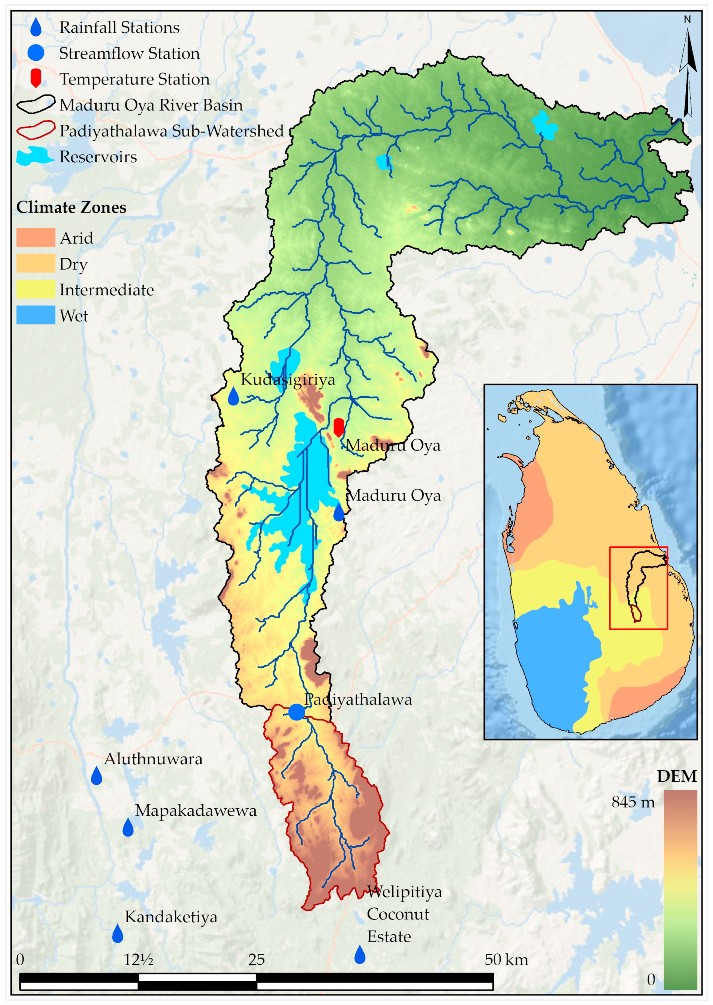
Figure 1. Padiyathalawa sub-watershed in Maduru Oya river basin.
Hydrology 11 00116 g001
Figure 2. Conceptual illustration of the Tank Model setup.
Hydrology 11 00116 g002
Figure 3. Sensitivity analysis of the Tank Model parameters for (A) peak flow and (B) first quartile (i.e., 25th percentile) flow. Note: A11-runoff coefficient to estimate surface flow, Z11-runoff hole depth to estimate surface flow, A12-runoff coefficient to estimate sub-surface flow, Z12-runoff hole depth to estimate sub-surface flow, B1-infiltration coefficient of the first tank, A2-runoff coefficient to estimate intermediate flow, Z2-runoff hole depth to estimate intermediate flow, B2-infiltration coefficient of the second tank, A3-runoff coefficient to estimate sub-base flow, Z3-runoff hole depth to estimate sub-base flow, B3-infiltration coefficient of the third tank, A4 runoff coefficient to estimate base flow.
Hydrology 11 00116 g003
Figure 4. Comparison of observed and simulated hydrographs (A) and flow-duration curves (B) at the basin outlet for the calibration period (between August 2011 and September 2012).
Hydrology 11 00116 g004
Figure 5. Comparison of observed and simulated hydrographs (A) and flow-duration curves (B) at the basin outlet for the validation period (between September 2015 and April 2016).
Hydrology 11 00116 g005
Figure 6. Variation of model performances (i.e., the King–Gupta Efficiency (KGE)) with weighted factor (ϑ) under multi-variable calibration.
Hydrology 11 00116 g006
Figure 7. Percentage change in Kling–Gupta Efficiency for streamflow ( K G E Q ) when the optimal parameters from multi-variable calibration are used in the simulation, compared to the simulations with parameters optimised from single-variable calibration (i.e., weighted factor (ϑ) of 0).
Hydrology 11 00116 g007
Figure 8. (A) Hydrograph and (B) FDCs for the Tank Model simulations (between September 2015 and April 2016) under calibration schemes with 0.1, 0.8, and 0.9 weighted factors (ϑ).
Hydrology 11 00116 g008
Figure 9. (A) Hydrograph and (B) FDCs for the Tank Model simulations (between August 2011 and September 2012) under validation schemes with 0.1, 0.8, and 0.9 weighted factors (ϑ).
Hydrology 11 00116 g009
Figure 10. Soil moisture simulation results under calibration schemes with 0.1, 0.8, and 0.9 weighted factors (ϑ) (between September 2015 and April 2016).
Hydrology 11 00116 g010
Table 2. Initial model parameters and their ranges.
Tank No.Model ParameterUnitInitial Value (Range)
1B1: infiltration coefficient of the first tank1/day0.23 (0–1)
A11: runoff coefficient to estimate surface flow1/day0.09 (0–1)
A12: runoff coefficient to estimate sub-surface flow1/day0.24 (0–1)
Z11: runoff hole depth to estimate surface flowmm2.89 (5–15)
Z12: runoff hole depth to estimate sub-surface flowmm38.77 (25–60)
2B2: infiltration coefficient of the second tank1/day0.02 (0–1)
A2: runoff coefficient to estimate intermediate flow1/day0.04 (0–1)
Z2: runoff hole depth to estimate intermediate flowmm78.38 (0–30)
3B3: infiltration coefficient of the third tank1/day0.01 (0–1)
A3: runoff coefficient to estimate sub-base flow1/day0.03 (0–1)
Z3: runoff hole depth to estimate sub-base flowmm1.89 (0–60)
4A4: runoff coefficient to estimate base flow1/day0.0001 (0–1)
Note: Initial parameter values were taken from Musiake and Wijesekera [60]; the minimum and maximum values of the model parameters were taken from Sugawara et al. [53].
Disclaimer/Publisher’s Note: The statements, opinions and data contained in all publications are solely those of the individual author(s) and contributor(s) and not of MDPI and/or the editor(s). MDPI and/or the editor(s) disclaim responsibility for any injury to people or property resulting from any ideas, methods, instructions or products referred to in the content.