1. Introduction
Underground water plays a key role in the hydrological cycle, and it is a very valuable resource for rivers and wetlands, especially during times of drought [
1]. As a result, the quality of the water must be taken into consideration. Groundwater contamination is the result of polluted water infiltrating through the soil and secondary porosity (fractures) in the rock and eventually reaching the groundwater [
2]. Because the water moves slowly through the soil, the impact on human activity is relatively long-term. Thus, pollution that occurred decades ago may still be dangerous presently for groundwater quality [
1]. The contamination of groundwater is a serious hazard because the pollutants may find their way into local agriculture products, either from the plants or animals, thus monitoring the concentration is of paramount importance. High concentrations of Cd can contribute to kidney damage or bone fragility and increase the chance of cancer. Exposure to high concentrations of Mn can contribute to neurological disorders and cognitive impairments in both humans and animals.
Mining has an impact on the quality of groundwater. The extent of the impact depends on a number of factors, such as the formation of the rock being mined, the type of soil, the technology used in mining, and the environmental commitment of each company [
3]. The mining process has expanded significantly in the past decades. Therefore, mining waste has multiplied, especially in opencast mines where excavations include large amounts of waste materials. Heavy metal pollution of water is caused when elements such as Cadmium, Lead, Arsenic, etc., come into contact with water. Groundwater contamination in heavy metals can affect the inhabited areas around the mine, not just the workers [
4].
Years of experience show that the measures employed are occasionally not adequate to remove all contaminants completely and that pollution sources, even if partially removed, continue to release pollutants. It is, therefore, preferable to prevent or reduce the risk of pollution rather than to deal with the consequences, and it is well-advised to have reliable estimations of the pollution in the entire area. Thus, the use of geostatistics in such environmental studies is both useful and important in order to guide the techniques used to reduce the pollution level [
5].
These reasons motivated our study of the potential contamination of groundwater in a mining area in Greece by the heavy metals Cd and Mn.
Similar works were performed by [
6], who used ordinary Kriging to analyze the spatial variability of pollutants in groundwater and [
7], who used ordinary Kriging (OK) to support groundwater quality management. Another application of OK by [
8] developed quality maps of pH, P, K, Ca and Mg in five Kentucky counties. Furthermore, Shi et al., 2007 [
9] analyzed 665 soil samples of Hg, Pd, Cu, As, Cr, and Cd. They applied OK and lognormal Kriging in order to create a map of their spatial patterns. Li et al., 2017 [
10] studied the spatial distribution and transport characteristics of heavy metals around a mine area in central China using OK.
Several recent studies on water quality monitoring were published recently, employing geostatistics. Barkat et al., 2021 [
11] assess the quality of groundwater both for drinking and irrigation purposes, using OK for the water quality index (WQI). Konaté et al., 2022 [
12] applied statistical and geostatistical methods to assess the problem of the quality of groundwater in the gold zone of Baraka, Republic of Guinea. Also, in 2022, Ngounouno Ayiwouo et al., 2022 [
13] used OK to trace metals (Fe, Mn, Cr, Ni, Cu, Zn and Pb) in surface sediments along the Lom River in the gold mining area of Gankombol. Last but not least, in 2020, Jianfei et al., 2020 [
14] searched for potential toxic elements in soils using absolute principal component score/multiple linear regression (APCS/MLR), positive matrix factorization (PMF) and geostatistics in a mining industry in Eastern China. The negative impact of mines in a river system in Australia is discussed by [
15], especially regarding the mobility of heavy elements. Zhang et al., 2023 [
16] used OK to investigate the distribution of heavy metal contaminants in a mining area in China. Zhu et al., 2019 [
17] used OK to estimate the distribution of pollutants in a mining area in southeastern China. Both works concluded that the distribution of pollutants was influenced by both natural factors (such as topography and soil properties) and anthropogenic factors (such as mining activities).
Compared to these works, the present paper focuses specifically on the estimation of water content in certain pollutants (Cd and Mn) and provides comparable and improved cross-validation metrics.
In the case of the mines of Northern Greece, the dataset and analysis present certain challenges that need to be overcome. The sample size is relatively small and the data locations are mainly clustered around the three mines Another issue is the presence of two dumping grounds for the tailings, areas where the concentration of pollutants is artificially increased in contrast with the underlying statistical stationarity assumption.
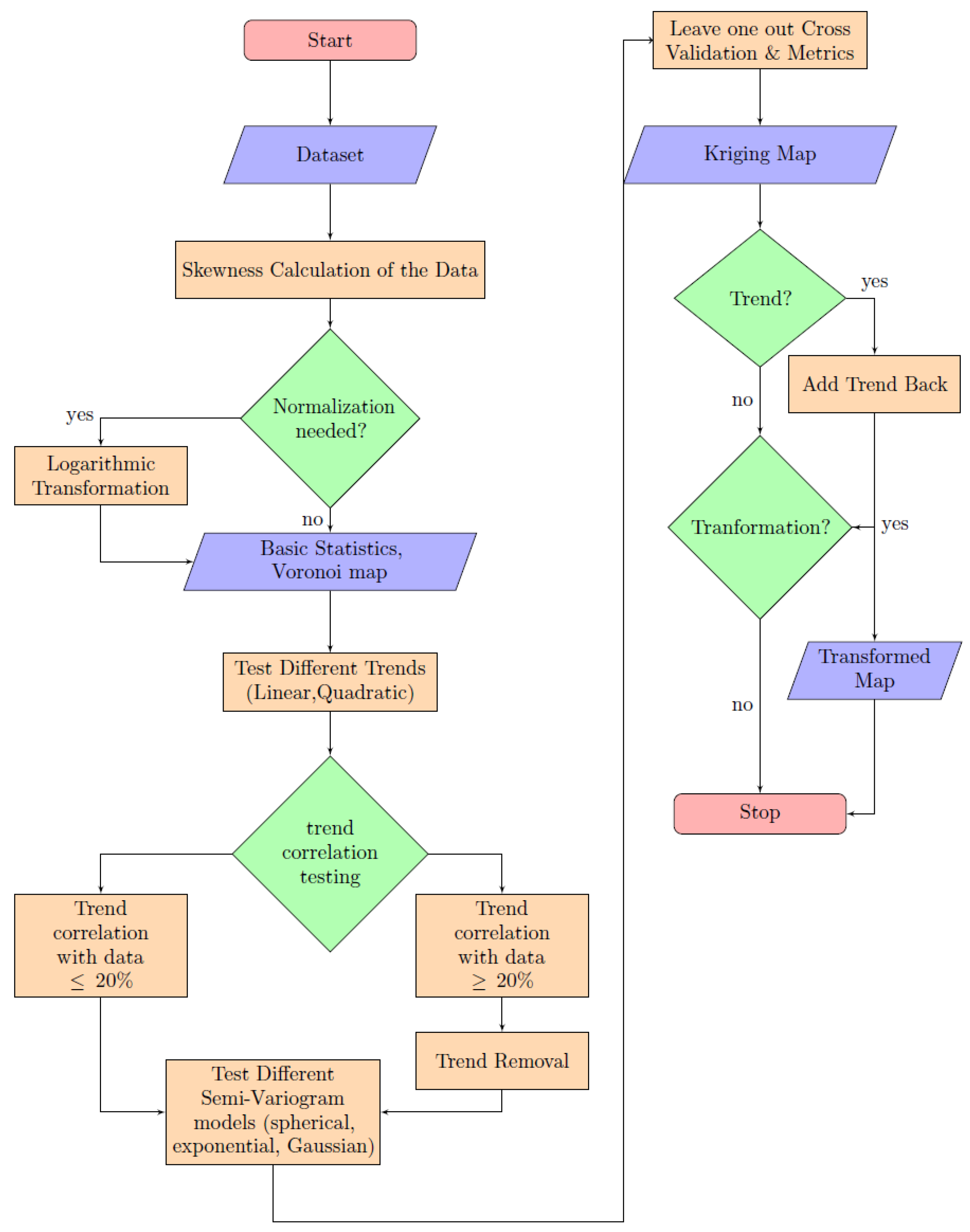
The analysis that follows is divided into four main stages: statistical analysis, trend investigation and removal, variography and ordinary Kriging. The flowchart of the procedure can be seen in
Figure 1. Discussion of the results and conclusions follows the geostatistical analysis.
2. Notation and General Principles
In the following analysis of the mine area dataset, we will make use of the following terms and principles. Random variable
X is a function whose domain of definition is a sampling frame
. The range of values is a set of real numbers
x. The capital letter
X will be used for the random variable while the lower case letter
x denotes a specific value of variable
X. The probability must be calculable for each value
x [
18].
In geostatistics, the term of the random field is commonly used. A random field is a random function, the value of which in every point in space is a different random variable. For simplicity, we can consider a random field as the collection of random variables in space.
In geostatistics a random field is considered to be composed of a deterministic part called the trend
and a stochastic part called Fluctuation
. The covariance function
shows how much the fluctuation of the point
depends on the point
. The function
of a random field
X(s) is defined in Equation (
1)
where
symbolizes the mathematical expectation, as in
In statistical homogeneous and isotropic fields, the key parameters of the covariance function are the variance
, the nugget effect
and correlation length (
h). Variance is the measure of the variation in the amplitude of the field. The correlation range
h normalizes the distance;
and defines the interval within which interdependence exists. The nugget effect (
) in the covariance model is a constant value for all distances greater than zero. It is affected by the volume of sampling, decreasing in value as the volume increases. It is related to the intrinsic randomness of the regionalized variable [
19].
The Mean Squared Error (MSE) is a measure of how close an estimation is to the data. It is the square of the error of the estimation (
, where
is the estimation). The greater the MSE, the worse the fit of the model. Another validation measure calculated is the Root Mean Squared Error (RMSE), which is the square root of the Mean Square Error. More than one validation measure is needed for the assessment of the quality and functionality of a geostatistical estimation [
18,
20].
2.1. Trend
The average values of the data are often related to the position in which they are located (spatially dependent) making the random field
X non-stationary. When the dependence of those random variables is fully known it can be described by deterministic functions [
19,
21]. Such a deterministic function describes the trend.
A random field
X is considered to be composed of the deterministic trend and the fluctuation as shown in
where
is the fluctuation of the random field around the
point [
18,
22].
Significant trends in the data should be removed in order to preserve stationarity [
23]. A trend can often be described as a linear or polynomial equation. For example, the first-order (linear) trend can be described by:
where
are the coordinates of a point
.
2.2. Variogram
The variogram of a random field is a measure of the spatial dependence between pairs of points. It is defined according to the following function:
where
is the distance vector and
is the mathematical expectation (the expected value) of the random field
X at the location
[
24].
In static homogeneous fields, the covariance and variogram functions are closely related [
25,
26]. Either one can be used for the calculation of spatial dependence as shown in
The empirical variogram equation of (
5) cannot calculate the variogram in any distance in space. It is thus required to fit a theoretical variogram model in order to have an approximation of the variogram value for all distances [
20].
Different variogram models have been tested in this research [
19]. One of the prevalent models selected after this analysis was the spherical variogram model presented in Equation (
7). This is a widely used model in spatial analysis that captures spatial correlation up to the correlation range
h, beyond which correlation becomes negligible.
The other model employed after the selection process was the Spartan Spatial Random Field (SSRF) model, detailed in Section Spartan Spatial Random Field.
Spartan Spatial Random Field
A novel covariance model, the Spartan Spatial Random Field (SSRF) was tested for the data in this analysis. The SSRF model is given by [
27]
In Equation (
8),
is the scale factor that determines the magnitude of the fluctuations,
is called the rigidity coefficient, and
is a normalization parameter that determines the range of spatial correlations. The remaining coefficients are given by
,
, and
. The range
h of the Spartan model is determined by both
and
. The SSRF model was shown to perform competitively in interpolation studies that involved coal mine reserves [
21] and groundwater level [
28] data. Furthermore, the SSRF model, thanks to its three parameters (
), can better adapt to a smaller amount of data [
27].
2.3. Kriging
Random field estimation attempts to predict the value of the field in locations for which no measurements have been made. The most widespread methods of linear interpolation belong to the family of Kriging [
26,
29]. Kriging methods are best linear unbiased estimators when the covariance (or variogram) of the field is known [
26].
In all Kriging methods, the predicted value of the study point is obtained by a weighted linear combination of the values of neighboring points. The weights are determined by minimizing the variance of error
(see
Section 2) using the covariance or variogram matrix [
20,
22].
In Kriging, a neighborhood is often employed. Neighborhood is around the prediction point , which includes points from . The size of the neighborhood is determined by the range h of the variogram as data outside are uncorrelated with the value of .
Kriging methods are the best linear unbiased estimators (BLUE) [
23]. Along with the lowest variance for the prediction error, Kriging methods provide the uncertainty of the estimation for each predicted location. For this study, ordinary Kriging (OK) is used. OK considers the trend as an unknown value that is constant within the neighborhood. In our case, the second-order trend has been removed but we opted to use OK instead of simple Kriging on the fluctuations in order to stabilize the residuals [
30].
The prediction of the field at the study point
is expressed by the linear combination shown in Equation (
9).
where
refers to the Kriging linear weights
. The weights are calculated with the help of the augmented covariance or variogram matrix
from Equation (
10)
with
,
being the lagrance coefficient and
the augmented variogram matrices shown in Equations (
11) and (
12) below:
One of the benefits of the Kriging method compared to deterministic methods is that the variance of the prediction can be calculated. If the data are close to the normal distribution, the Kriging variance
corresponds to a normal distribution of values around the predicted value. Thus, for Gaussian data, Kriging methods do not provide just the estimated value but the entire distribution allowing for confidence intervals of the prediction [
18,
19,
31]. Thus, OK can provide a measure of the uncertainty of the estimation. For OK, the variance of the prediction is given by
The logarithm of the concentrations of the elements in the investigated dataset is not sufficiently close to the normal distribution as shown in
Table 1. Thus, the Kriging variance
does not correspond to a normal distribution around the predicted value
.
3. Study Area and Prelimenary Analysis
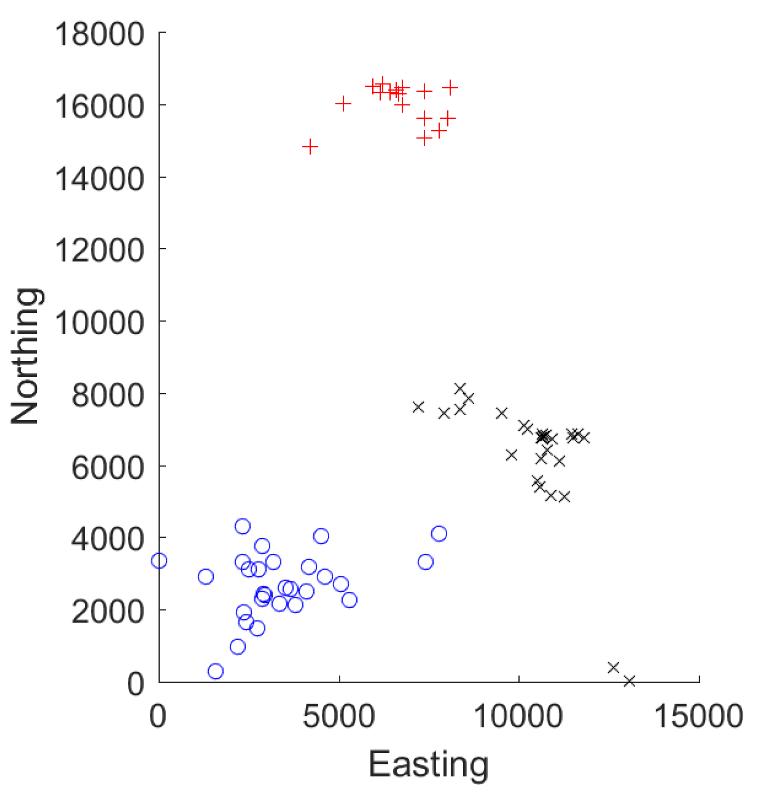
The study area contains three mines, with the locations shown in
Figure 2. The coordinates of the axes (easting and northing) have been adjusted so that the value of 0 on each axis corresponds to the minimum observed coordinate value. i.e., the easting of the westernmost sampling location equals
and the northing of the southmost sampling location equals
. Distances are in meters. One of the mines is currently inactive and the company is trying to reduce the environmental footprint of the mines in the region [
32].
The area is geologically composed of various metamorphic and igneous rocks; biotite gneisses with intercalations of marble horizons are located in the area, and granodiorites and acid to intermediate sub-volcanic rock intrusions into the gneisses cover small areas. The study area is characterized hydrogeologically as semi-permeable, and its vertical profile comprises three hydrostratigraphic units. Secondary porosity (fractures) is responsible for hydrological connectivity. In certain areas, the rocks exhibit strong fragmentation which increases with depth, thus creating pathways for slow groundwater flow. Government and company studies in the area have shown that the water reservoirs are connected [
32].
Our study was carried out by using geostatistical methods to determine the spatial variability of the quality of underground water in the area of these three mines.
The data are comprised of concentrations of Cd and Mn pollutants in the water samples at the 62 locations shown in
Figure 2. As the data did not follow the normal distribution, the logarithmic transform was applied in order for the distribution of the data values to be closer to the normal distribution. When using logarithms of the data or other non-linear transformations, care must be taken to investigate whether the transformation leads to biased estimations, and if necessary use bias correction methods similar to those presented in [
19]. The value of Kriging prediction is not affected by the distribution of the data. However, Kriging variance depends on the distribution, making it unreliable in skewed data sets. Furthermore, the potential for error is expected to be greater at a prediction point surrounded by data with very different values from a point surrounded by data with a smoother variation in local values [
31,
33]. Thus, a distribution closer to the normal distribution is desired.
3.1. Data Statistics
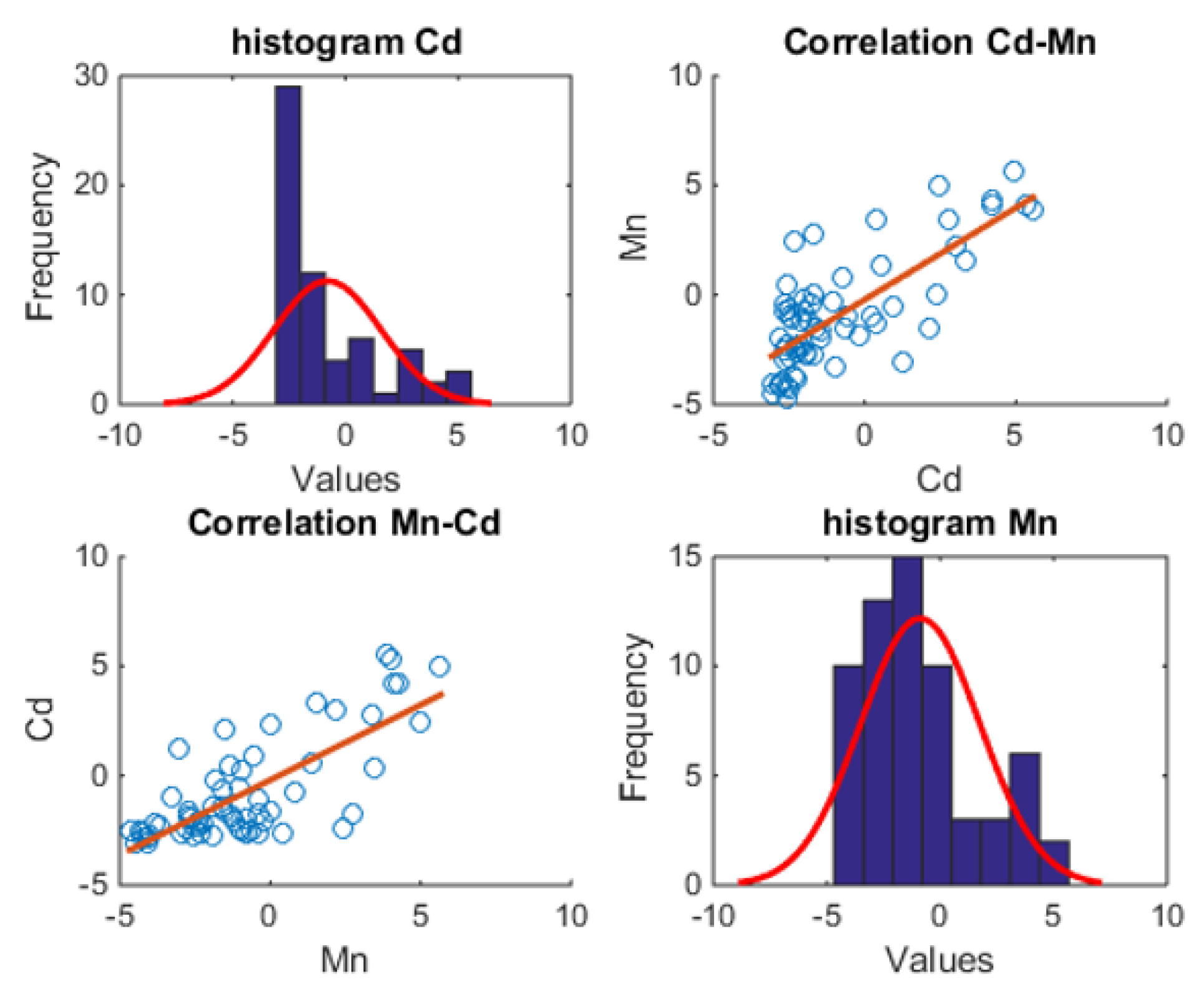
Table 1 shows the basic statistics of the Cd and Mn elements after logarithmic transformations. The small number of the dataset did not allow for any attempts at declustering.
The histograms representing the data of each element and the correlation between them are presented in
Figure 3. The correlation between the values of Cd and Mn is 54% in the entire area. Thus, there is a medium to strong correlation between the values of Cd and Mn in space. After the logarithmic transformation, the data are still skewed. However, as shown in
Table 1 and the histograms of
Figure 3, the logarithm values have a range of
to
for Cd and
to
for Mn. Compared to the unaltered range of 0.05 ppb to 261.65 ppb for Cd and 1.60 ppm to 289.46 ppm for Mn, Kriging smoothing is expected to affect the predictions less dramatically, producing lower errors [
33].
3.2. Trend Analysis
As mentioned in
Section 2.1, existing trends within the data can lead to spatial dependencies in the data and thus non-stationarity. Preliminary investigation with a linear trend model (first-order polynomial trend) has shown that a low-order polynomial was not sufficient for adequate removal of the trend. Thus, a second-order polynomial was removed as shown in Equation (
14).
where the polynomial coefficients are shown in
Table 2.
are the coordinates for
.
We decided to estimate the trend and its coefficients through multi-linear regression [
33]. The correlation coefficient with second-order trend for the element Cd is equal to 45.70%, while in Mn is equal to 63.76%. As a rule of thumb, a trend with a correlation over 20% should be removed from the data or it will cause issues in the model estimations of the stochastic part of the random field (the fluctuation
) [
21,
24].
3.3. Variogram Models for Cd, Mn
In order to select the variogram model for each investigated element, the fluctuations in the data
have been used to estimate the empirical variogram at 10 lags (Cd) and 11 lags (Mn). Different variogram models have been tested for this purpose. We used least squares error to fit the various theoretical models (exponential, Gaussian, spherical, SSRF) to the empirical variogram and extract the model parameters [
24].
The spherical variogram model of Equation (
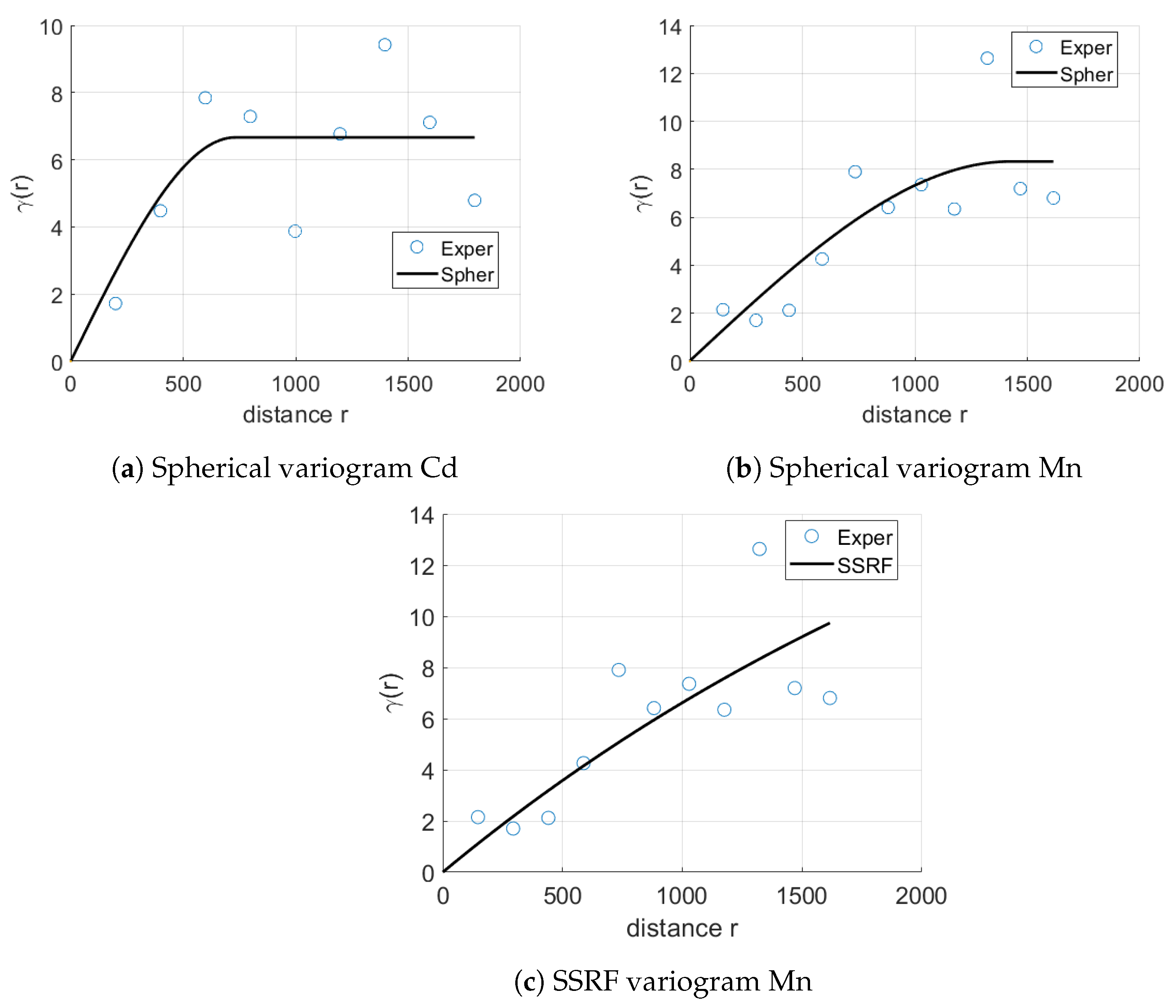
7) was found to provide the best fit by returning the lowest least squares error for the element of Cd. The spherical variogram is fit to the experimental variogram as shown in
Figure 4a,b. The range
h is the maximum distance of spatial dependence and
is the variance.
For Cd (
Figure 4a), the range
h is just 731 m, which means points are correlated in a distance of 731 m. As such, reliable measurements of Cd are possible only at a short distance from the boreholes. The variance for Cd is
.
For the Mn element, shown in
Figure 4c, the results are more promising since the distance of the dependence is larger at
m. The other parameters of the Spartan Variogram model are:
. The Spherical Variogram is presented in
Figure 4b for comparison. The parameters of the Spherical variogram are
m,
.
5. Discussion
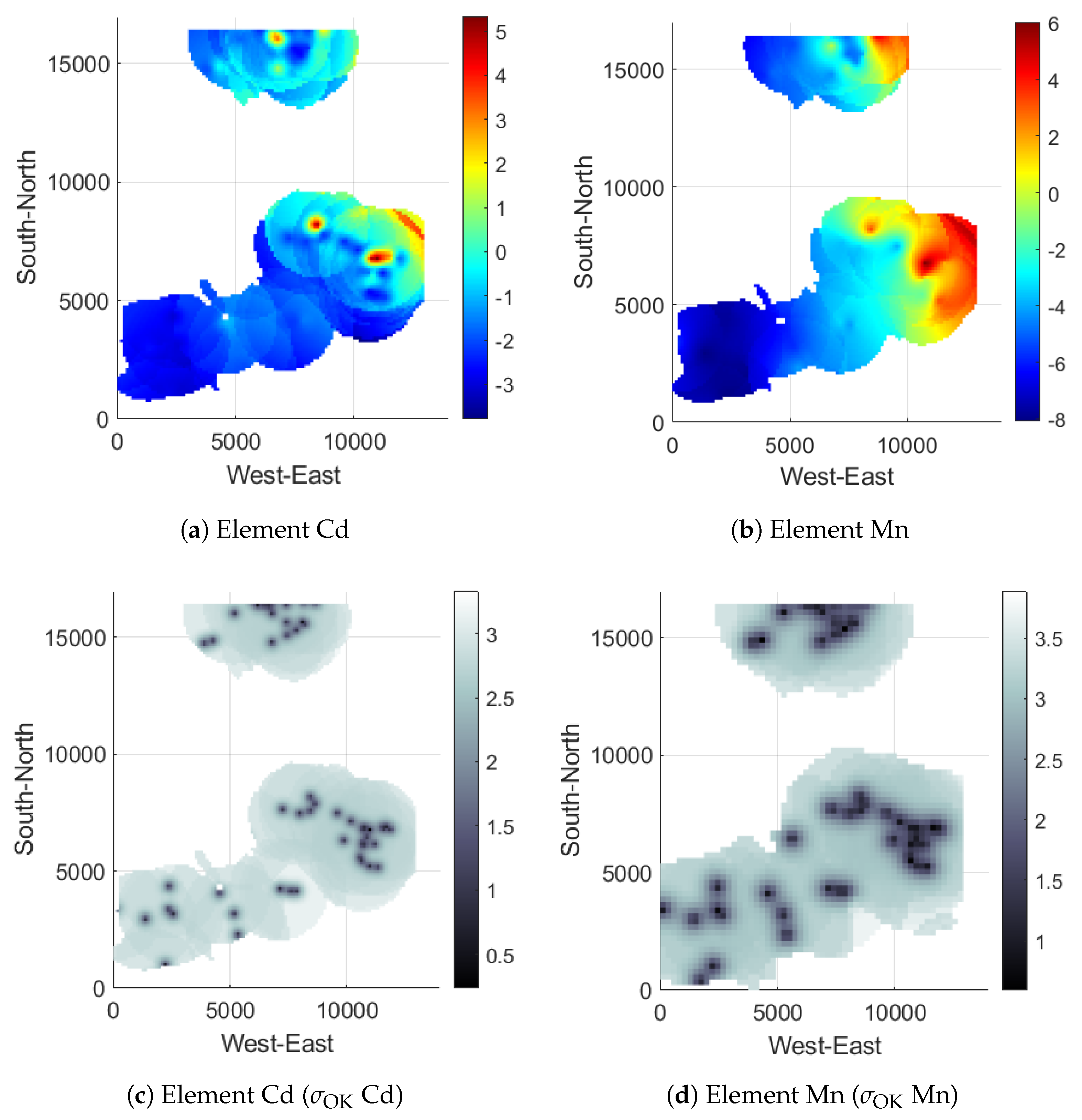
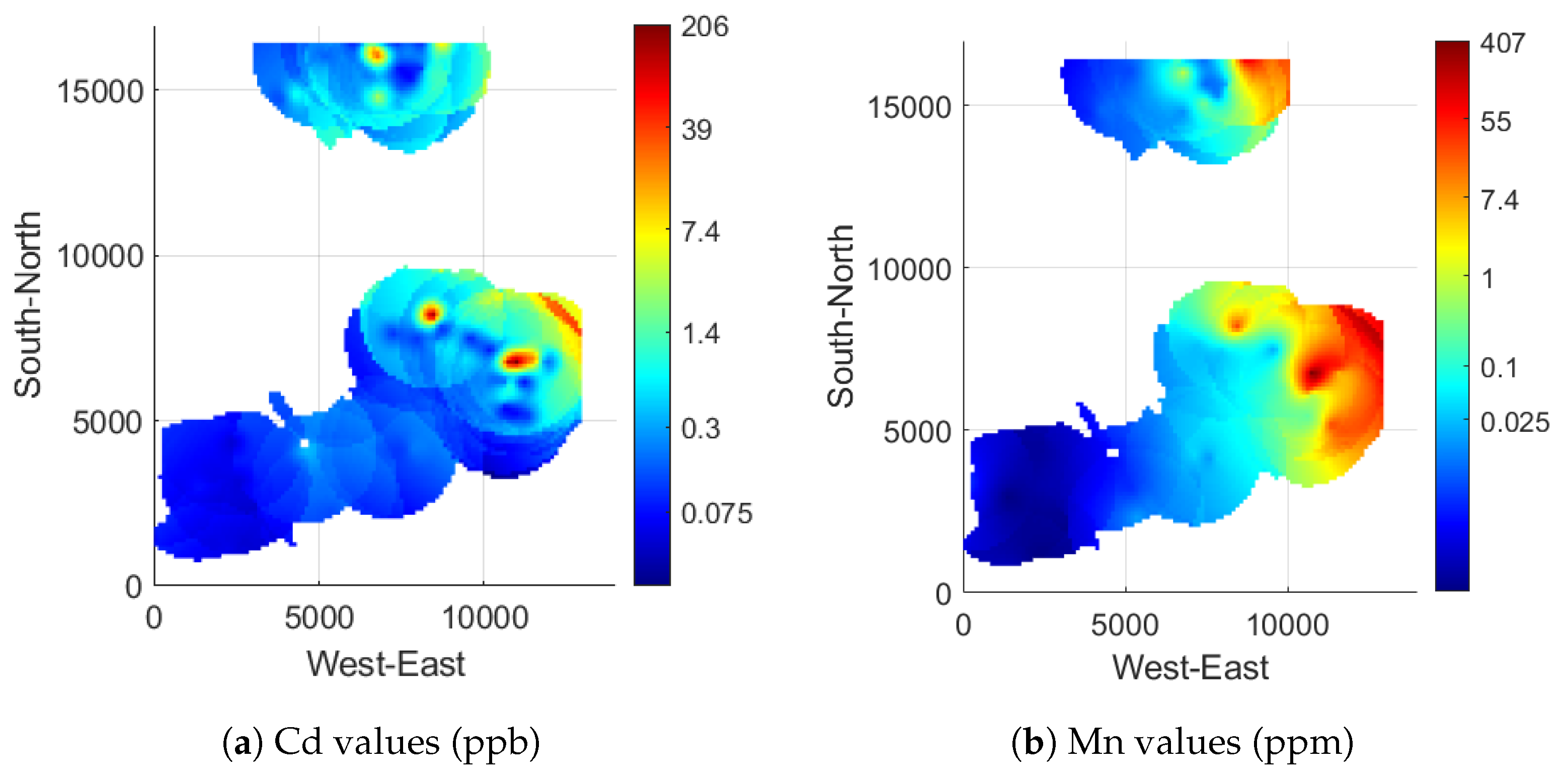
There are several works in the literature that have used geostatistical prediction methods to estimate contamination in mining sites. We investigated the correlation between Cd and Mn and used the logarithm of the data values to estimate the variogram parameters and compared widely used variogram models (spherical, exponential, Gaussian) with the SSRF variogram model. We employed OK to create contamination prediction maps that better represent the values of Cd and Mn. The cross-validation outcomes were encouraging, demonstrating that the prediction maps are representative.
The choice to remove a second-order polynomial trend was reached after preliminary analysis showed there was a significant trend in the data. After removing the first-order polynomial trend, variogram analysis showed that a significant trend remained in the data. The variogram would not reach a sill, which, according to [
19,
33], represents the non-stationarity introduced by trend. Thus, a second-order trend was removed. The trend’s coefficient was estimated using multilinear regression [
22].
The cross-validation results of
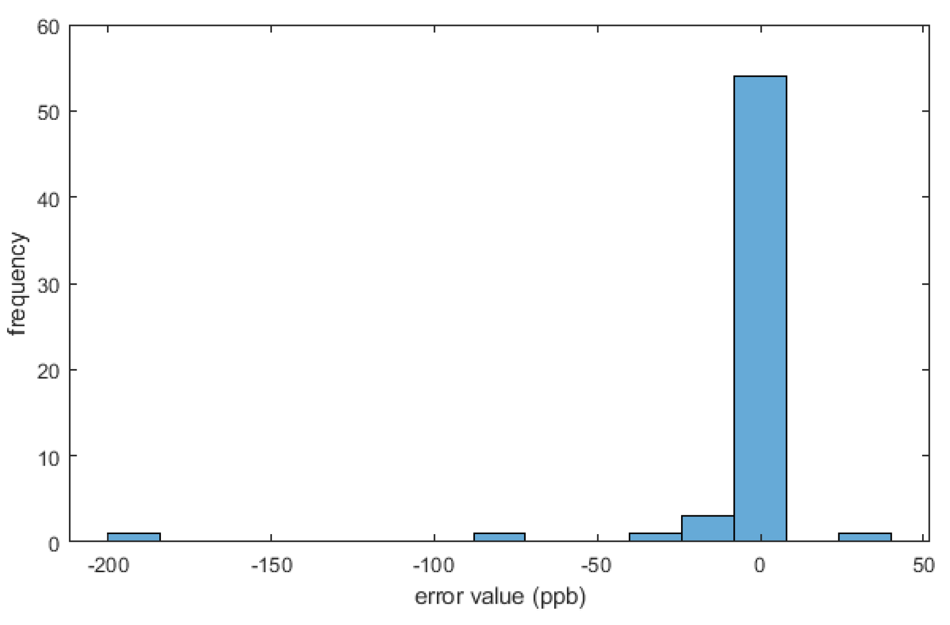
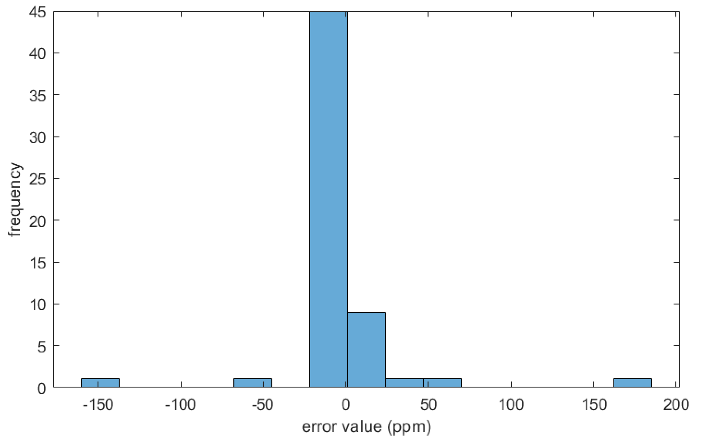
Table 3 show promising results with a correlation of 0.65 for Cd and 0.52 for Mn, and root mean squared error (RMSE) of 25.9 ppb for Cd and 25.1 ppm for Mn. These results indicate that the prediction maps based on the best-fit model parameters are reasonably accurate. It should be noted that without the Bias correction, the errors were more significant for both elements. For the element of Cd, without bias correction, MaxAE = 194 ppb, mean error = −5 ppb, and
. Mn displayed less bias (ME = 1.7 ppm) but the improvement was still noticeable. Without bias correction, the validation measures for Mn were MaxAE = −182 ppm, RMSE = 32.6 ppm and
. This noticeable improvement for both elements showcases the benefits of the bias correction of Equation (
17).
The exception for both elements, locations where cross-validation did not perform well are locations near the dumping grounds of the tailings from the mining activities. LOOCV predicts the value of location based on surrounding values. Thus, significantly high concentrations that are non-stationary, have this effect, as it is impossible for Kriging methods to predict a value of 400 ppm for Mn or 200 ppb for Cd based on surrounding values of 2 to 40 ppm, resulting in high errors in such locations. However, the prediction map incorporates all data, including the outliers; thus, predictions around the location of the tailings are accurate. The quick drop in the concentration of the pollutant in drill-holes away from the tailing areas shows the extend of the influence of the dumping grounds in space. Thus, such methods can be useful for monitoring and managing contamination during mining activities.
The SSRF variogram detailed in Section Spartan Spatial Random Field was tested for both Cd and Mn. While the Spherical was found to give a better fit and better LOOCV results for Cd, the SSRF variogram showed significant improvement for the Mn predictions as shown in
Table 3. It is also worth mentioning that while the spherical variogram predictions for both Cd and Mn returned right-skewed errors, with the highest error being an underestimation of the concentration in the dumping grounds, the SSRF for Mn (see
Figure 8 is more symmetrical. The highest error was again an underestimation of the value at the dumping grounds.
Another issue encountered in this analysis was the small amount of available data. It has been shown in studies [
27] that the SSRF variogram can better adapt to a smaller amount of data. Despite the small sample size, which includes outliers (the dumping grounds), SSRF was able to give a fair prediction for Mn concentration, showing that it can capture the complex spatial dependencies well despite the small sample size.
6. Conclusions
In this study, spatial analysis with OK is used to present the contamination of groundwater in two heavy elements, Cd and Mn, for an area of mining activity. High concentrations of Cd and Mn in the water increase the risk of environmental damage and impact the health of humans and animals in the area. The systematic monitoring that the local mining company performs, helps to observe any contamination and take appropriate measures if necessary. The spatial distribution of the pollutants can assist companies in focusing their attention on areas that have high concentrations. The range of the variogram can help to define the extent of the spread of the contamination. Namely, one of the locations used as a dumping ground for tailings has been announced as the place for a restoration project by local authorities to protect the environment and the surrounding area.
Overall, the use of geostatistical prediction methods in mining and environmental management is a well-established area of research. The present paper contributes to this area by presenting a case study of the application of geostatistical analysis to estimate water content in certain pollutants in a group of mines in Northern Greece.
The data values were transformed (logarithm) to better approach the normal distribution. The data are scattered and divided among three mines in the area. A second-order trend has been removed. However, issues with field stationarity persist because of the presence of dumping grounds with higher concentrations. According to LOOCV results (see
Table 3), the most accurate results are obtained on Cd although estimation for the concentration of both elements was satisfactory with the exception of dumping grounds, which are considered outliers.
The results presented in the paper demonstrate the successful use of geostatistical prediction methods to estimate the water content of certain pollutants. The cross-validation results show promising results with a correlation of 0.65 for Cd and 0.52 for Mn, and root mean squared error (RMSE) of 25.9 ppb for Cd and 25.1 ppm for Mn. These results indicate that the prediction maps, based on the best-fit model parameters, are reasonably accurate with the exception of a few artifacts at the eastern edge of the mines. Thus, such methods can be useful for monitoring and managing contamination during mining activities. From the various variogram models tested, the SSRF model was shown to significantly improve the predictions for Mn compared to the spherical model.
The authors used the original Matlab code to apply the method of OK to create contamination prediction maps that better represent the values of Cd and Mn, which are important contaminants that need to be monitored during mining activities.
As a direction for future studies, the uncertainty of the predictions could be further investigated. As mentioned in
Section 4.2 the logarithmic transformation presents challenges. By means of kernel-based Gaussian anamorphosis [
31,
35], the probability distribution of the sample can be transformed to the normal distribution. Thus, the prediction uncertainty could be assessed using conditional simulations [
21,
25,
31]. To further explore the uncertainty introduced by the estimation of the trend, universal Kriging could be applied to the data [
18,
22].
