
Evaluating Best Management Practice Efficacy Based on Seasonal Variability and Spatial Scales

 , , , and
Abstract
1. Introduction
2. Materials and Methods
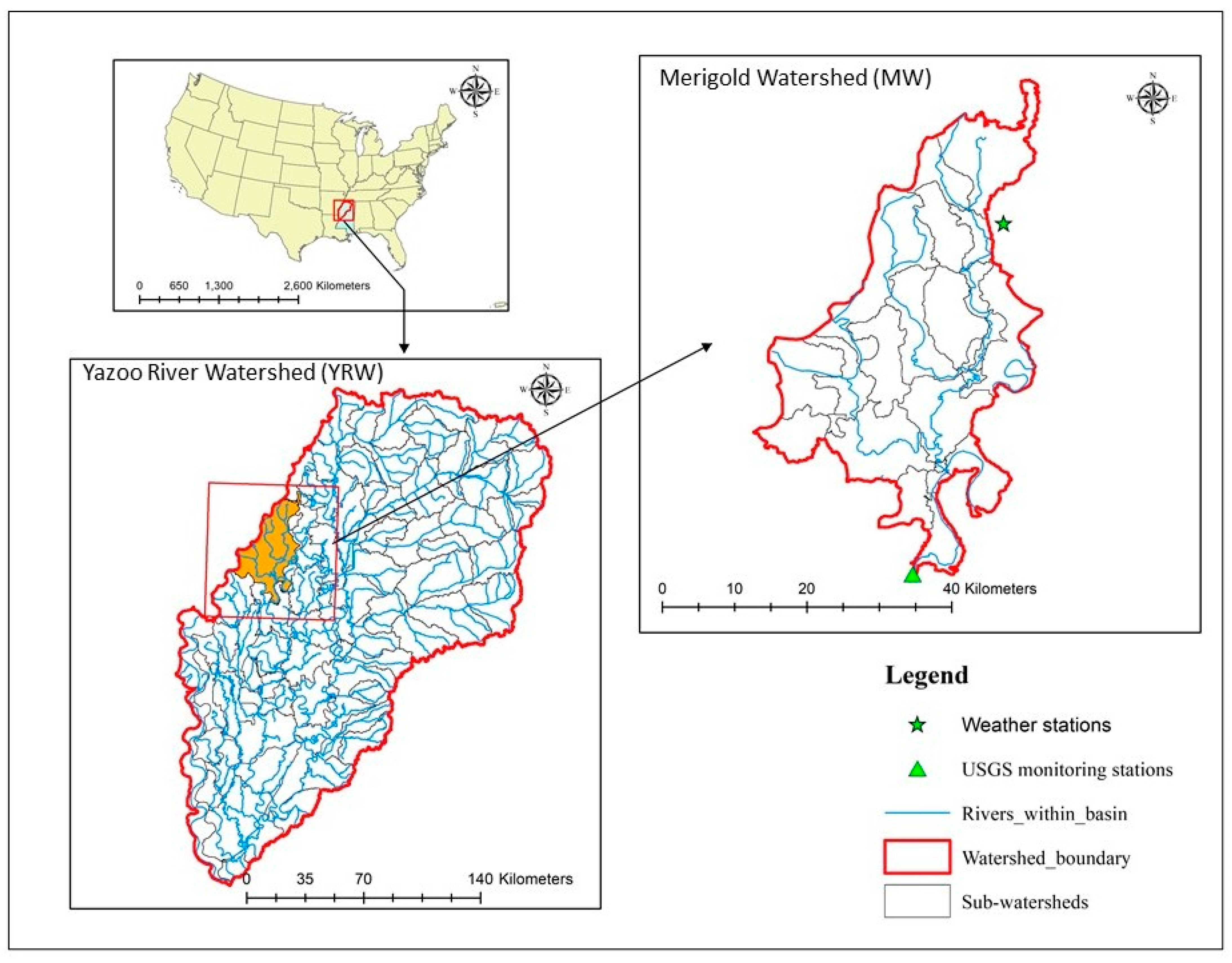
2.1. Study Area
2.2. Model Description and Data Inputs
2.3. Data Inputs
2.4. Model Accuracy Assessment
2.5. Seasonal Variation and Management Scenarios
2.5.1. Vegetative Filter Strips (VFSs)
2.5.2. Cover Crops (CCs)
3. Results
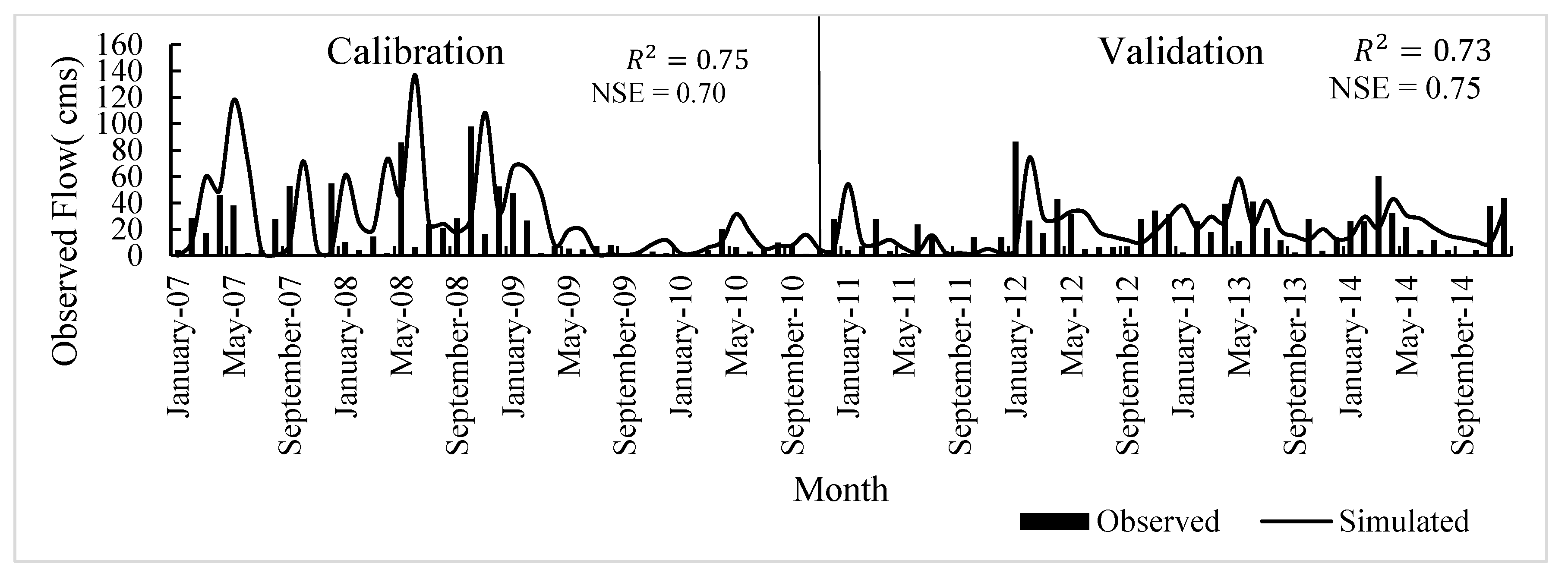
3.1. Model Accuracy Assessment
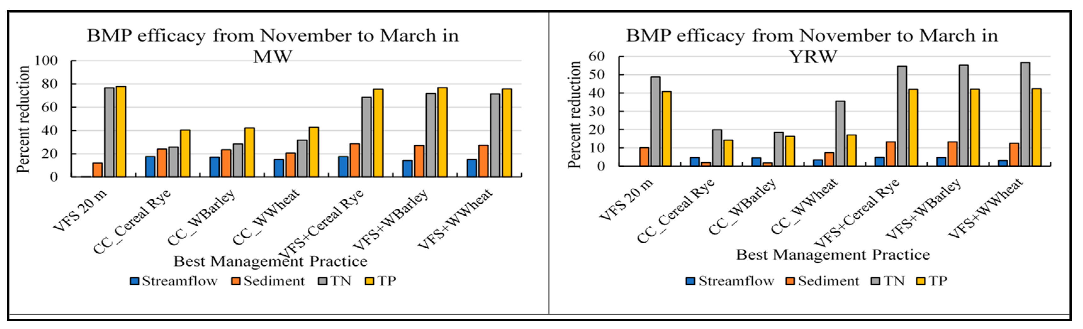
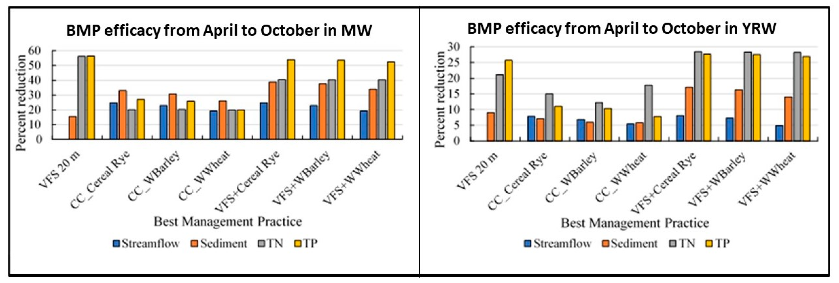
3.2. Seasonal Variation in the Efficacy of BMPs
4. Discussion
5. Conclusions
Author Contributions
Funding
Data Availability Statement
Conflicts of Interest
References
- US-EPA. Water Conservation at EPA|US EPA. 2023. Available online: https://www.epa.gov/greeningepa/water-conservation-epa (accessed on 2 May 2023).
- US EPA. National Water Quality Inventory: Report to Congress, Washington DC. 2017. Available online: https://www.epa.gov/national-aquatic-resource-surveys (accessed on 2 May 2023).
- Lacher, I.L.; Ahmadisharaf, E.; Fergus, C.; Akre, T.; Mcshea, W.J.; Benham, B.L.; Kline, K.S. Scale-dependent impacts of urban and agricultural land use on nutrients, sediment, and runoff. Sci. Total Environ. 2019, 652, 611–622. [Google Scholar] [CrossRef] [PubMed]
- Dash, P.; Silwal, S.; Ikenga, J.O.; Pinckney, J.L.; Arslan, Z.; Lizotte, R.E. Water Quality of Four Major Lakes in Mississippi, USA: Impacts on Human and Aquatic Ecosystem Health. Water 2015, 7, 4999–5030. [Google Scholar] [CrossRef]
- Shaughnessy, A.R.; Sloan, J.J.; Corcoran, M.J.; Hasenmueller, E.A. Sediments in Agricultural Reservoirs Act as Sinks and Sources for Nutrients over Various Timescales. Water Resour. Res. 2019, 55, 5985–6000. [Google Scholar] [CrossRef]
- Diebel, M.W.; Maxted, J.T.; Nowak, P.J.; Zanden, M.J.V. Landscape Planning for Agricultural Nonpoint Source Pollution Reduction I: A Geographical Allocation Framework. Environ. Manag. 2008, 42, 789–802. [Google Scholar] [CrossRef] [PubMed]
- Bhattarai, S.; Parajuli, P.B. Best Management Practices Affect Water Quality in Coastal Watersheds. Sustainability 2023, 15, 4045. [Google Scholar] [CrossRef]
- Nepal, D.; Parajuli, P.B. Assessment of Best Management Practices on Hydrology and Sediment Yield at Watershed Scale in Mississippi Using SWAT. Agriculture 2022, 12, 518. [Google Scholar] [CrossRef]
- Feng, G.; Cobb, S.; Abdo, Z.; Fisher, D.K.; Ouyang, Y.; Adeli, A.; Jenkins, J.N. Trend analysis and forecast of precipitation, reference evapotranspiration, and rainfall deficit in the blackland prairie of eastern Mississippi. J. Appl. Meteorol. Climatol. 2016, 55, 1425–1439. [Google Scholar] [CrossRef]
- USDA-NASS. United States Department of Agriculture National Agricultural Statistics Service Mississippi Crop Production, Jackson, MS. 2022. Available online: https://www.nass.usda.gov/ms (accessed on 2 May 2023).
- Nearing, M.A.; Yin, S.Q.; Borrelli, P.; Polyakov, V.O. Rainfall erosivity: An historical review. CATENA 2017, 157, 357–362. [Google Scholar] [CrossRef]
- Vanrobaeys, J.A.; Owens, P.N.; Lobb, D.A.; Kieta, K.A.; Campbell, J.M. Seasonal Efficacy of Vegetated Filter Strips for Phosphorus Reduction in Surface Runoff. J. Environ. Qual. 2019, 48, 880–888. [Google Scholar] [CrossRef]
- Roley, S.S.; Tank, J.L.; Tyndall, J.C.; Witter, J.D. How cost-effective are cover crops, wetlands, and two-stage ditches for nitrogen removal in the Mississippi River Basin? Water Resour. Econ. 2016, 15, 43–56. [Google Scholar] [CrossRef]
- Elçi, A. Evaluation of Nutrient Retention in Vegetated Filter Strips Using the SWAT Model. In Proceedings of the WA 2nd Regional Symposium on Water, Wastewater and Environment, Çesme-Izmir, Turkey, 22–24 March 2017; Available online: https://www.researchgate.net/publication/315716174 (accessed on 2 May 2023).
- Her, Y.; Chaubey, I.; Frankenberger, J.; Smith, D. Effect of conservation practices implemented by USDA programs at field and watershed scales. J. Soil Water Conserv. 2016, 71, 249–266. [Google Scholar] [CrossRef]
- Karki, R.; Srivastava, P.; Bosch, D.D.; Kalin, L.; Lamba, J.; Strickland, T.C. Multi-Variable Sensitivity Analysis, Calibration, and Validation of a Field-Scale SWAT Model: Building Stakeholder Trust in Hydrologic and Water Quality Modeling. Trans. ASABE 2020, 63, 523–539. [Google Scholar] [CrossRef]
- Merriman, K.R.; Daggupati, P.; Srinivasan, R.; Toussant, C.; Russell, A.M.; Hayhurst, B. Assessing the impact of site-specific BMPs using a spatially explicit, field-scale SWAT model with edge-of-field and tile hydrology and water-quality data in the Eagle Creek Watershed, Ohio. Water 2018, 10, 1299. [Google Scholar] [CrossRef]
- Risal, A.; Parajuli, P.B. Evaluation of the Impact of Best Management Practices on Streamflow, Sediment and Nutrient Yield at Field and Watershed Scales. Water Resour. Manag. 2022, 36, 1093–1105. [Google Scholar] [CrossRef]
- Guse, B.; Kail, J.; Radinger, J.; Schröder, M.; Kiesel, J.; Hering, D.; Wolter, C.; Fohrer, N. Eco-hydrologic model cascades: Simulating land use and climate change impacts on hydrology, hydraulics and habitats for fish and macroinvertebrates. Sci. Total Environ. 2015, 533, 542–556. [Google Scholar] [CrossRef] [PubMed]
- Arnold, J.G.; Srinivasan, R.; Muttiah, R.S.; Williams, J.R. Large area hydrologic modeling and assessment part I: Model development. J. Am. Water Resour. Assoc. 1998, 34, 73–89. [Google Scholar] [CrossRef]
- Abbaspour, K.C.; Vaghefi, S.A.; Srinivasan, R. A guideline for successful calibration and uncertainty analysis for soil and water assessment: A review of papers from the 2016 international SWAT conference. Water 2017, 10, 6. [Google Scholar] [CrossRef]
- Addab, H.; Bailey, R.T. Simulating the effect of subsurface tile drainage on watershed salinity using SWAT. Agric. Water Manag. 2022, 262, 107431. [Google Scholar] [CrossRef]
- Bacu, V.; Mihon, D.; Rodila, D.; Stefanut, T.; Gorgan, D. gSWAT platform for grid based hydrological model calibration and execution. In Proceedings of the 2011 10th International Symposium on Parallel and Distributed Computing, Cluj-Napoca, Romania, 6–8 July 2011; pp. 288–291. [Google Scholar] [CrossRef]
- Dakhlalla, A.O.; Parajuli, P.B. Assessing model parameters sensitivity and uncertainty of streamflow, sediment, and nutrient transport using SWAT. Inf. Process. Agric. 2019, 6, 61–72. [Google Scholar] [CrossRef]
- Maski, D.; Mankin, K.R.; Anand, S.; Janssen, K.A.; Pierzynski, G.M. Calibration and Validation of SWAT for Field-Scale Sediment-Yield Prediction. In Proceedings of the Annual International Meeting, Portland, Oregon, 9–12 July 2006; American Society of Agricultural and Biological Engineers: St. Joseph, MI, USA, 2006. [Google Scholar] [CrossRef]
- Du, J.; Rui, H.; Zuo, T.; Li, Q.; Zheng, D.; Chen, A.; Xu, Y.; Xu, C.Y. Hydrological Simulation by SWAT Model with Fixed and Varied Parameterization Approaches Under Land Use Change. Water Resour. Manag. 2013, 27, 2823–2838. [Google Scholar] [CrossRef]
- Ouyang, Y.; Feng, G.; Parajuli, P.; Leininger, T.; Wan, Y.; Jenkins, J.N. Assessment of Surface Water Quality in the Big Sunflower River Watershed of Mississippi Delta Using Nonparametric Analysis. Water. Air. Soil Pollut. 2018, 229, 373. [Google Scholar] [CrossRef] [PubMed]
- Sinnathamby, S.; Douglas-Mankin, K.R.; Craige, C. Field-scale calibration of crop-yield parameters in the Soil and Water Assessment Tool (SWAT). Agric. Water Manag. 2017, 180, 61–69. [Google Scholar] [CrossRef]
- AgnKowalczyk, W.; Grabowska-Polanowska, B.; Garbowski, T.; Kopacz, M.; Lach, S.; Mazur, R. A multicriteria approach to different land use scenarios in the Western Carpathians with the SWAT model. J. Water Land Dev. 2023, 57, 130–139. [Google Scholar] [CrossRef]
- Abdullaeva, B.S. Integrating advanced approaches for climate change impact assessment on water resources in arid regions. J. Water Land Dev. 2024, 60, 149–156. [Google Scholar] [CrossRef]
- Johnson, T.; Butcher, J.; Deb, D.; Faizullabhoy, M.; Hummel, P.; Kittle, J.; Mcginnis, S.; Mearns, L.O.; Nover, D.; Parker, A.; et al. Modeling Streamflow and Water Quality Sensitivity to Climate Change and Urban Development in 20 U.S. Watersheds. J. Am. Water Resour. Assoc. 2015, 51, 1321–1341. [Google Scholar] [CrossRef] [PubMed]
- Paul, M.; Rajib, M.A.; Ahiablame, L. Spatial and Temporal Evaluation of Hydrological Response to Climate and Land Use Change in Three South Dakota Watersheds. J. Am. Water Resour. Assoc. 2017, 53, 69–88. [Google Scholar] [CrossRef]
- Shrestha, S.; Bhatta, B.; Shrestha, M.; Shrestha, P.K. Integrated assessment of the climate and landuse change impact on hydrology and water quality in the Songkhram River Basin, Thailand. Sci. Total Environ. 2018, 643, 1610–1622. [Google Scholar] [CrossRef] [PubMed]
- Risal, A.; Parajuli, P.B. Quantification and simulation of nutrient sources at watershed scale in Mississippi. Sci. Total Environ. 2019, 670, 633–643. [Google Scholar] [CrossRef]
- Neupane, R.P.; Kumar, S. Estimating the effects of potential climate and land use changes on hydrologic processes of a large agriculture dominated watershed. J. Hydrol. 2015, 529, 418–429. [Google Scholar] [CrossRef]
- NOAA. Statewide Rankings|Climate at a Glance|National Centers for Environmental Information (NCEI). 2023. Available online: https://www.ncei.noaa.gov/access/monitoring/climate-at-a-glance/statewide/rankings/22/pcp/201912 (accessed on 3 May 2023).
- Zhang, B.; Feng, G.; Read, J.J.; Kong, X.; Ouyang, Y.; Adeli, A.; Jenkins, J.N. Simulating soybean productivity under rainfed conditions for major soil types using APEX model in East Central Mississippi. Agric. Water Manag. 2016, 177, 379–391. [Google Scholar] [CrossRef]
- Feng, G.; Ouyang, Y.; Adeli, A.; Read, J.; Jenkins, J. Rainwater Deficit and Irrigation Demand for Row Crops in Mississippi Blackland Prairie. Soil Sci. Soc. Am. J. 2018, 82, 423–435. [Google Scholar] [CrossRef]
- Anapalli, S.S.; Reddy, K.N.; Jagadamma, S. Conservation tillage impacts and adaptations in irrigated corn production in a humid climate. Agron. J. 2018, 110, 2673–2686. [Google Scholar] [CrossRef]
- Blanco-Canqui, H.; Ruis, S.J.; Holman, J.D.; Creech, C.F.; Obour, A.K.; Blanco-Canqui, C.H. Can cover crops improve soil ecosystem services in water-limited environments? A review. Soil Sci. Soc. Am. J. 2021, 86, 1–18. [Google Scholar] [CrossRef]
- Abdalla, M.; Hastings, A.; Cheng, K.; Yue, Q.; Chadwick, D.; Espenberg, M.; Truu, J.; Rees, R.M.; Smith, P. A critical review of the impacts of cover crops on nitrogen leaching, net greenhouse gas balance and crop productivity. Glob. Chang. Biol. 2019, 25, 2530–2543. [Google Scholar] [CrossRef] [PubMed]
- Lassaletta, L.; Billen, G.; Grizzetti, B.; Anglade, J.; Garnier, J. 50 year trends in nitrogen use efficiency of world cropping systems: The relationship between yield and nitrogen input to cropland. Environ. Res. Lett. 2014, 9, 105011. [Google Scholar] [CrossRef]
- Badon, T.; Czarnecki, J.M.P.; Baker, B.H.; Spencer, D.; Hill, M.J.; Lucore, A.E.; Krutz, L.J. Transitioning from conventional to cover crop systems with minimum tillage does not alter nutrient loading. J. Environ. Qual. 2022, 51, 966–977. [Google Scholar] [CrossRef] [PubMed]
- Baker, B.; Omer, A.; Oldham, L.; Burger, L.M.D. Natural Resources Conservation in Agriculture, Mississippi State University Extension, Mississippi State, MS. 2017. Available online: https://www.researchgate.net/publication/318363028 (accessed on 3 May 2023).
- Firth, A.G.; Brooks, J.P.; Locke, M.A.; Morin, D.J.; Brown, A.; Baker, B.H. Dynamics of Soil Organic Carbon and CO2 Flux under Cover Crop and No-Till Management in Soybean Cropping Systems of the Mid-South (USA). Environments 2022, 9, 109. [Google Scholar] [CrossRef]
- Venishetty, V.; Parajuli, P.B.; Nepal, D. Spatial Variability of Best Management Practices Effectiveness on Water Quality within the Yazoo River Watershed. Hydrology 2023, 10, 92. [Google Scholar] [CrossRef]
- Liu, Y.; Engel, B.A.; Flanagan, D.C.; Gitau, M.W.; McMillan, S.K.; Chaubey, I.; Singh, S. Modeling framework for representing long-term effectiveness of best management practices in addressing hydrology and water quality problems: Framework development and demonstration using a Bayesian method. J. Hydrol. 2018, 560, 530–545. [Google Scholar] [CrossRef]
- Arnold, J.G.; Williams, J.R.; Maidment, D.R. Continuous-Time Water and Sediment-Routing Model for Large Basins. J. Hydraul. Eng. 1995, 121, 171–183. [Google Scholar] [CrossRef]
- Williams, J.R.; Berndt, H.D. Sediment Yield Prediction Based on Watershed Hydrology. Trans. ASAE 1977, 20, 1100–1104. [Google Scholar] [CrossRef]
- Knisel, W.; Nicls, A. CREAMS—A Field Scale Model for Chemicals, Runoff, and Erosion from Agricultural Management Systems, Washington DC. 1980. Available online: https://www.google.com/books/edition/CREAMS/AwcUAAAAYAAJ?hl=en&gbpv=1&dq=CREAMS:+a+field+scale+model+for+chemicals,+runoff+and+erosion+from+agricultural+management+systems.+USDASEA+Conservation,+Research+Report&pg=PA1&printsec=frontcover (accessed on 16 December 2022).
- Leonard, R.A.; Knisel, W.G.; Still, D.A. GLEAMS: Groundwater Loading Effects of Agricultural Management Systems. Trans. ASAE 1987, 30, 1403–1418. [Google Scholar] [CrossRef]
- De Mello, C.R.; Norton, L.D.; Pinto, L.C.; Beskow, S.; Curi, N. Agricultural watershed modeling: A review for hydrology and soil erosion processes. Ciência Agrotecnologia 2016, 40, 7–25. [Google Scholar] [CrossRef]
- USGS. Digital Elevation Models. 2020. Available online: https://apps.nationalmap.gov/downloader/#productSearch (accessed on 27 August 2020).
- Pignotti, G.; Rathjens, H.; Cibin, R.; Chaubey, I.; Crawford, M. Comparative Analysis of HRU and Grid-Based SWAT Models. Water 2017, 9, 272. [Google Scholar] [CrossRef]
- Sliwi´nski, D.; Konieczna, A.; Roman, K. Geostatistical Resampling of LiDAR-Derived DEM in Wide Resolution Range for Modelling in SWAT: A Case Study of Zgłowiączka River (Poland). Remote Sens. 2022, 14, 1281. [Google Scholar] [CrossRef]
- USDA-NASS. USDA—National Agricultural Statistics Service—Research & Science—Cropland Data Layer—Metadata. 2009. Available online: https://www.nass.usda.gov/Research_and_Science/Cropland/metadata/meta.php (accessed on 25 April 2023).
- NRCS. Web Soil Survey (WSS) SSURGO Database. 2012. Available online: https://websoilsurvey.sc.egov.usda.gov/App/WebSoilSurvey.aspx (accessed on 10 September 2020).
- NOAA. National Oceanic and Atmospheric Administration (NOAA) Climate Data Online (CDO)|National Climatic Data Center (NCDC). 2019. Available online: https://www.ncdc.noaa.gov/cdo-web/search (accessed on 31 August 2020).
- MAFES. Mississippi Agricultural and Forestry Experiment Station—Variety Trials. 2006. Available online: https://www.mafes.msstate.edu/variety-trials/ (accessed on 31 August 2020).
- JNash, E.; Sutcliffe, J.V. River flow forecasting through conceptual models part I—A discussion of principles. J. Hydrol. 1970, 10, 282–290. [Google Scholar] [CrossRef]
- Legates, D.R.; McCabe, G.J. Evaluating the use of “goodness-of-fit” measures in hydrologic and hydroclimatic model validation. Water Resour. Res. 1999, 35, 233–241. [Google Scholar] [CrossRef]
- Abbaspour, K.C.; Johnson, C.A.; van Genuchten, M.T. Estimating Uncertain Flow and Transport Parameters Using a Sequential Uncertainty Fitting Procedure. Vadose Zone J. 2004, 3, 1340–1352. [Google Scholar] [CrossRef]
- USGS. USGS Daily, Monthly and Yearly Data for Mississippi: Stage and Streamflow. 2002. Available online: https://waterdata.usgs.gov/ms/nwis/current/?type=dailystagedischarge&group_key=basin_cd#Equipment_malfunction (accessed on 10 August 2020).
- US-EPA. Guidance for Quality Assurance Project Plans for Modeling EPA QA/G-5M, Washington, DC. 2002. Available online: www.epa.gov/quality (accessed on 22 March 2023).
- Venishetty, V.; Parajuli, P.B. Assessment of BMPs by Estimating Hydrologic and Water Quality Outputs Using SWAT in Yazoo River Watershed. Agriculture 2022, 12, 477. [Google Scholar] [CrossRef]
- Maharjan, G.R.; Ruidisch, M.; Shope, C.L.; Choi, K.; Huwe, B.; Kim, S.J.; Tenhunen, J.; Arnhold, S. Assessing the effectiveness of split fertilization and cover crop cultivation in order to conserve soil and water resources and improve crop productivity. Agric. Water Manag. 2016, 163, 305–318. [Google Scholar] [CrossRef]
- Berkowitz, J.F.; Schlea, D.A.; VanZomeren, C.M.; Boles, C.M.W. Coupling watershed modeling, public engagement, and soil analysis improves decision making for targeting P retention wetland locations. J. Great Lakes Res. 2020, 46, 1331–1339. [Google Scholar] [CrossRef]
- Teshager, A.D.; Gassman, P.W.; Secchi, S.; Schoof, J.T. Simulation of targeted pollutant-mitigation-strategies to reduce nitrate and sediment hotspots in agricultural watershed. Sci. Total Environ. 2017, 607–608, 1188–1200. [Google Scholar] [CrossRef]
- Getahun, E.; Keefer, L.L. Assessing the Effectiveness of Winter Cover Crops for Controlling Agricultural Nutrient Losses. J. Am. Water Resour. Assoc. 2023, 59, 510–522. [Google Scholar] [CrossRef]
- NRCS. United States Department of Agriculture—Natural Resources Conservation Service (USDA-NRCS) Filter Strip|NRCS. 2016. Available online: https://www.nrcs.usda.gov/wps/portal/nrcs/detail/national/landuse/rangepasture/?cid=nrcs142p2_044352 (accessed on 5 December 2021).
- Neitsch, S.L.; Arnold, J.G.; Kiniry, J.R.; Williams, J.R. Soil and Water Assessment Tool Theoretical Documentation Version 2009; College of Agriculture and Life Sciences—Texas A&M University: College Station, TX, USA, 2011. [Google Scholar]
- Arnold, J.G.; Moriasi, D.N.; Gassman, P.W.; Abbaspour, K.C.; White, M.J.; Srinivasan, R.; Santhi, C.; Harmel, R.D.; Van Griensven, A.; Van Liew, M.W.; et al. SWAT: Model use, Calibration, and Validation. Trans. ASABE 2012, 55, 1491–1508. [Google Scholar] [CrossRef]
- Luo, Y. Modeling the Mitigating Effects of Conservation Practices for Pyrethroid Uses in Agricultural Areas of California. ACS Symp. Ser. 2019, 1308, 275–289. [Google Scholar] [CrossRef]
- USDA-NRCS. United States Department of Agriculture—Natural Resources Conservation Service (USDA-NRCS)—Cover Crop|NRCS, Washington DC. 2014. Available online: https://www.nrcs.usda.gov/sites/default/files/2022-09/Cover_Crop_340_CPS.pdf (accessed on 20 December 2020).
- LaRose, J.; Myers, R. Cover Crops: A Cost-Effective Tool for Controling Erosion, Columbia, MO. 2021. Available online: https://cra.missouri.edu/wp-content/uploads/2021/09/Cover-crops-controlling-erosion.pdf (accessed on 3 May 2023).
- Burdine, B. Cover Crops: Benefits and Limitations; Mississippi State University Extension Service: Verona, MS, USA, 2019. [Google Scholar]
- Moriasi, D.N.; Arnold, J.G.; Van Liew, M.W.; Bingner, R.L.; Harmel, R.D.; Veith, T.L. Model Evaluation guidelines for Systematic quantification of Accuracy in Watershed simulations. Trans. ASABE 2007, 50, 885–900. [Google Scholar] [CrossRef]
- Wallace, C.W.; Flanagan, D.C.; Engel, B.A. Evaluating the Effects of Watershed Size on SWAT Calibration. Water 2018, 10, 898. [Google Scholar] [CrossRef]
- Abbaspour, K.C.; Rouholahnejad, E.; Vaghefi, S.; Srinivasan, R.; Yang, H.; Kløve, B. A continental-scale hydrology and water quality model for Europe: Calibration and uncertainty of a high-resolution large-scale SWAT model. J. Hydrol. 2015, 524, 733–752. [Google Scholar] [CrossRef]
- Jalowska, A.M.; Yuan, Y. Evaluation of SWAT Impoundment Modeling Methods in Water and Sediment Simulations. J. Am. Water Resour. Assoc. 2019, 55, 209–227. [Google Scholar] [CrossRef]
- Santhi, C.; Arnold, J.G.; Williams, J.R.; Hauck, L.M.; Dugas, W.A. Application of a watershed model to evaluate management effects on point and nonpoint source pollution. Trans. ASAE 2001, 44, 1559–1570. [Google Scholar] [CrossRef]
- Yuan, Y.; Chiang, L.C. Sensitivity analysis of SWAT nitrogen simulations with and without in-stream processes. Arch. Agron. Soil Sci. 2014, 61, 969–987. [Google Scholar] [CrossRef]
- Sommerlot, A.R.; Nejadhashemi, A.P.; Woznicki, S.A.; Prohaska, M.D. Evaluating the impact of field-scale management strategies on sediment transport to the watershed outlet. J. Environ. Manag. 2013, 128, 735–748. [Google Scholar] [CrossRef] [PubMed]
- Sharpley, A.N.; Kleinman, P.J.; Jordan, P.; Bergström, L.; Allen, A.L. Evaluating the Success of Phosphorus Management from Field to Watershed. J. Environ. Qual. 2009, 38, 1981–1988. [Google Scholar] [CrossRef] [PubMed]
- Rittenburg, R.A.; Squires, A.L.; Boll, J.; Brooks, E.S.; Easton, Z.M.; Steenhuis, T.S. Agricultural BMP effectiveness and dominant hydrological flow paths: Concepts and a review. J. Am. Water Resour. Assoc. 2015, 51, 305–329. [Google Scholar] [CrossRef]
- USDA NRCS. Conservation Effects Assessment Project (CEAP) Assessment of the Effects of Conservation Practices on Cultivated Cropland in the Lower Mississippi River Basin, Washington, DC. 2013. Available online: http://www.nrcs.usda.gov/technical/nri/ceap/ (accessed on 15 December 2021).
- Malone, R.W.; Kersebaum, K.C.; Kaspar, T.C.; Ma, L.; Jaynes, D.B.; Gillette, K. Winter rye as a cover crop reduces nitrate loss to subsurface drainage as simulated by HERMES. Agric. Water Manag. 2017, 184, 156–169. [Google Scholar] [CrossRef]
- Nouri, A.; Lee, J.; Yin, X.; Tyler, D.D.; Saxton, A.M. Thirty-four years of no-tillage and cover crops improve soil quality and increase cotton yield in Alfisols, Southeastern USA. Geoderma 2019, 337, 998–1008. [Google Scholar] [CrossRef]
- Muñoz-Carpena, R.; Ritter, A.; Bosch, D.D.; Schaffer, B.; Potter, T.L. Summer cover crop impacts on soil percolation and nitrogen leaching from a winter corn field. Agric. Water Manag. 2008, 95, 633–644. [Google Scholar] [CrossRef]
- Gabriel, J.L.; Quemada, M.; Martín-Lammerding, D.; Vanclooster, M. Assessing the cover crop effect on soil hydraulic properties by inverse modelling in a 10-year field trial. Agric. Water Manag. 2019, 222, 62–71. [Google Scholar] [CrossRef]
- De Cima, D.S.; Luik, A.; Reintam, E. Organic farming and cover crops as an alternative to mineral fertilizers to improve soil physical properties. Int. Agrophysics 2015, 29, 405–412. [Google Scholar] [CrossRef]
- Hudek, C.; Putinica, C.; Otten, W.; De Baets, S. Functional root trait-based classification of cover crops to improve soil physical properties. Eur. J. Soil Sci. 2022, 73, e13147. [Google Scholar] [CrossRef]
- Pokhrel, S.; Kingery, W.L.; Cox, M.S.; Shankle, M.W.; Shanmugam, S.G. Impact of Cover Crops and Poultry Litter on Selected Soil Properties and Yield in Dryland Soybean Production. Agronomy 2021, 11, 119. [Google Scholar] [CrossRef]
- Adeli, A.; Read, J.J.; Brooks, J.P.; Miles, D.; Feng, G.; Jenkins, J.N. Broiler Litter × Industrial By-Products Reduce Nutrients and Microbial Losses in Surface Runoff When Applied to Forages. J. Environ. Qual. 2017, 46, 339–347. [Google Scholar] [CrossRef] [PubMed]
- Hu, J.; Miles, D.M.; Adeli, A.; Brooks, J.P.; Podrebarac, F.A.; Smith, R.; Lei, F.; Li, X.; Jenkins, J.N.; Moorhead, R.J. Effects of Cover Crops and Soil Amendments on Soil CO2 Flux in a Mississippi Corn Cropping System on Upland Soil. Environments 2023, 10, 19. [Google Scholar] [CrossRef]


| Process | Sediment | TN | TP | |||
|---|---|---|---|---|---|---|
| R2 | NSE | R2 | NSE | R2 | NSE | |
| Calibration (2014) | 0.20 | 0.17 | 0.15 | 0.18 | 0.30 | 0.35 |
| Validation (2015) | 0.23 | 0.21 | 0.14 | 0.20 | 0.47 | 0.42 |
| November to March (Wet Season) | Best Management Practices (BMPs) | Percent Reduction | |||
|---|---|---|---|---|---|
| Streamflow | Sediment | TN | TP | ||
| Merigold Watershed | VFS 20 m | 0.05 | 12.00 | 76.70 | 77.70 |
| CC_Cereal Rye | 17.53 | 24.10 | 25.84 | 40.45 | |
| CC_WBarley | 17.00 | 23.34 | 28.43 | 42.21 | |
| CC_WWheat | 15.00 | 20.56 | 31.66 | 42.77 | |
| VFS + Cereal Rye | 17.54 | 28.72 | 68.46 | 75.50 | |
| VFS + WBarley | 14.19 | 27.05 | 71.67 | 76.74 | |
| VFS + WWheat | 15.00 | 27.25 | 71.41 | 75.63 | |
| Yazoo River Watershed | VFS 20 m | 0.00 | 10.13 | 48.75 | 40.79 |
| CC_Cereal Rye | 4.79 | 2.04 | 19.94 | 14.29 | |
| CC_WBarley | 4.57 | 1.86 | 18.47 | 16.34 | |
| CC_WWheat | 3.51 | 7.35 | 35.53 | 17.05 | |
| VFS + Cereal Rye | 4.91 | 13.40 | 54.66 | 42.00 | |
| VFS + WBarley | 4.79 | 13.36 | 55.20 | 42.15 | |
| VFS + WWheat | 3.17 | 12.54 | 56.65 | 42.32 | |
| April to October (Dry Season) | Best Management Practices (BMPs) | Percent Reduction | |||
|---|---|---|---|---|---|
| Streamflow | Sediment | TN | TP | ||
| Merigold Watershed | VFS 20 m | 0.12 | 15.50 | 56.10 | 56.30 |
| CC_Cereal Rye | 24.64 | 33.00 | 20.09 | 27.00 | |
| CC_WBarley | 22.84 | 30.61 | 20.24 | 25.75 | |
| CC_WWheat | 19.19 | 26.00 | 19.82 | 20.01 | |
| VFS + Cereal Rye | 24.64 | 38.88 | 40.42 | 53.83 | |
| VFS + WBarley | 22.84 | 37.64 | 40.20 | 53.40 | |
| VFS + WWheat | 19.19 | 33.89 | 40.30 | 52.35 | |
| Yazoo River Watershed | VFS 20 m | 0.00 | 9.02 | 21.16 | 25.72 |
| CC_Cereal Rye | 7.84 | 7.11 | 15.00 | 11.00 | |
| CC_WBarley | 6.84 | 5.97 | 12.26 | 10.39 | |
| CC_WWheat | 5.42 | 5.84 | 17.77 | 7.73 | |
| VFS + Cereal Rye | 8.02 | 17.10 | 28.47 | 27.64 | |
| VFS + WBarley | 7.29 | 16.34 | 28.31 | 27.54 | |
| VFS + WWheat | 4.88 | 14.04 | 28.22 | 26.93 | |
Disclaimer/Publisher’s Note: The statements, opinions and data contained in all publications are solely those of the individual author(s) and contributor(s) and not of MDPI and/or the editor(s). MDPI and/or the editor(s) disclaim responsibility for any injury to people or property resulting from any ideas, methods, instructions or products referred to in the content. |
© 2024 by the authors. Licensee MDPI, Basel, Switzerland. This article is an open access article distributed under the terms and conditions of the Creative Commons Attribution (CC BY) license (https://creativecommons.org/licenses/by/4.0/).
Share and Cite
Venishetty, V.; Parajuli, P.B.; To, F.; Nepal, D.; Baker, B.; Gude, V.G. Evaluating Best Management Practice Efficacy Based on Seasonal Variability and Spatial Scales. Hydrology 2024, 11, 58. https://doi.org/10.3390/hydrology11040058
Venishetty V, Parajuli PB, To F, Nepal D, Baker B, Gude VG. Evaluating Best Management Practice Efficacy Based on Seasonal Variability and Spatial Scales. Hydrology. 2024; 11(4):58. https://doi.org/10.3390/hydrology11040058
Chicago/Turabian StyleVenishetty, Vivek, Prem B. Parajuli, Filip To, Dipesh Nepal, Beth Baker, and Veera Gnaneswar Gude. 2024. "Evaluating Best Management Practice Efficacy Based on Seasonal Variability and Spatial Scales" Hydrology 11, no. 4: 58. https://doi.org/10.3390/hydrology11040058
APA StyleVenishetty, V., Parajuli, P. B., To, F., Nepal, D., Baker, B., & Gude, V. G. (2024). Evaluating Best Management Practice Efficacy Based on Seasonal Variability and Spatial Scales. Hydrology, 11(4), 58. https://doi.org/10.3390/hydrology11040058