Article

MODIS Evapotranspiration Forecasting Using ARIMA and ANN Approach at a Water-Stressed Irrigation Scheme in South Africa

by
Mbulelo Phesa
1,*,
Nkanyiso Mbatha
2 and
Akinola Ikudayisi
1
1
Department of Civil Engineering, Walter Sisulu University, East London 5201, South Africa
2
Department of Geography and Environmental Studies, University of Zululand, KwaDlangezwa 3886, South Africa
*
Author to whom correspondence should be addressed.
Hydrology 2024, 11(10), 176; https://doi.org/10.3390/hydrology11100176
Submission received: 8 September 2024 / Revised: 3 October 2024 / Accepted: 15 October 2024 / Published: 21 October 2024

Abstract

:
The forecasting of evapotranspiration (ET) in some water-stressed regions remains a major challenge due to the lack of reliable and sufficient historical datasets. For efficient water balance, ET remains the major component and its proper forecasting and quantifying is of the utmost importance. This study utilises the 18-year (2001 to 2018) MODIS ET obtained from a drought-affected irrigation scheme in the Eastern Cape Province of South Africa. This study conducts a teleconnection evaluation between the satellite-derived evapotranspiration (ET) time series and other related remotely sensed parameters such as the Normalised Difference Vegetation Index (NDVI), Normalised Difference Water Index (NDWI), Normalised Difference Drought Index (NDDI), and precipitation (P). This comparative analysis was performed by adopting the Mann–Kendall (MK) test, Sequential Mann–Kendall (SQ-MK) test, and Multiple Linear Regression methods. Additionally, the ET detailed time-series analysis with the Keiskamma River streamflow (SF) and monthly volumes of the Sandile Dam, which are water supply sources close to the study area, was performed using the Wavelet Analysis, Breaks for Additive Seasonal and Trend (BFAST), Theil–Sen statistic, and Correlation statistics. The MODIS-obtained ET was then forecasted using the Autoregressive Integrated Moving Average (ARIMA) and Artificial Neural Networks (ANNs) for a period of 5 years and four modelling performance evaluations such as the Root Mean Square Error (RMSE), Mean Absolute Percentage Error (MAPE), Mean Absolute Error (MAE), and the Pearson Correlation Coefficient (R) were used to evaluate the model performances. The results of this study proved that ET could be forecasted using these two time-series modeling tools; however, the ARIMA modelling technique achieved lesser values according to the four statistical modelling techniques employed with the RMSE for the ARIMA = 37.58, over the ANN = 44.18; the MAE for the ARIMA = 32.37, over the ANN = 35.88; the MAPE for the ARIMA = 17.26, over the ANN = 24.26; and for the R ARIMA = 0.94 with the ANN = 0.86. These results are interesting as they give hope to water managers at the irrigation scheme and equally serve as a tool to effectively manage the irrigation scheme.

1. Introduction

Evapotranspiration (ET) is the simultaneous loss of water from plants and soil surfaces to the atmosphere. The process takes place in two phases, the evaporation of water from the ground and the transpiration of water from plants. Evaporation is the transmission of water from the soil, canopy intervention, and water bodies, whilst transpiration is water loss from plants through holes in the leaves (Phesa, Woyessa [1]). It is responsible for returning more than 60% of precipitation back into the atmosphere; therefore, ET is regarded as the second-largest hydrological flux after precipitation [2]. Furthermore, ET is the main variable for agricultural water balance; thus, the prediction of water balance is key for irrigation schemes’ management, regulation, and effective agricultural water resources planning.
The proper modeling of ET further assists in mitigating water scarcity, leads to the formation of a sustainable water balance, and avoids the unnecessary waste and overuse of water resources [3]. To forecast ET, the Penman–Monteith (PM) equation is a widely used technique; however, it is very hard to obtain all the relevant data in developing countries like South Africa; thus, reliable alternative and effective modeling techniques are employed to evaluate non-linear trends linked to ET predictor variables [1]. Satellite-based evapotranspiration was forecasted in a data-scarce region in Ethiopia and the results indicated that remote sensing helps to fine-tune hydrological models [4]. Due to the lack of data in Brazil, remote sensing data were employed and the results were successful in forecasting ET [5]. Many other studies [6,7,8,9] show that the Keskammahoek irrigation scheme does not only suffer from limited data availability for the proper estimation of ET, but the region has been suffering from a multi-year drought [10].
According to Graw, Ghazaryan [11], the entirety of the Eastern Cape Province has experienced severe droughts over the last 10 years based on the lower correlation between vegetation indices, and precipitation. Other hydrological parameters are also assessed in this study in order to gain an understanding of ET over the study area. ET is one of the key components of the hydrological cycle and its accurate forecasting along with other variables is very important for water resources management, environmental conversation, and agricultural planning, and further providing a comprehensive understanding of water availability and distribution [12]. The Normalised Difference Vegetation Index (NDVI), Normalised Difference Water Index (NDWI), and Normalised Difference Drought Index (NDDI) have a distinct connection with ET as they reflect different aspects of the land surface that influence the ET rate [13]. Furthermore, the precipitation over the study area is also assessed because of its strong interconnection with ET. Precipitation is a primary source of water for ET, so, when precipitation falls, it can infiltrate the soil, replenish the soil moisture, or accumulate on the plant surface [14]. Based on the study by Li, Cheng [15], the connection between river streamflow and ET is a fundamental aspect of the hydrological cycle. Evapotranspiration reduces the amount of water available for streamflow by returning moisture to the atmosphere. This interaction is influenced by various factors, including vegetation cover, land use, climate conditions, and groundwater dynamics.
Therefore, understanding and managing the balance between ET and streamflow is crucial for sustainable water resource management, especially in the face of climate change and increasing water demands [16]. Equally, ET has a direct impact on the supply dam; therefore, Sandile dam volumes close to the study area were also assessed. ET has a significant impact on the dam levels as it directly affects water availability in a watershed that contributes to the inflow and storage in the dams [17]. Likewise, forecasting ET in a water-stressed region can be particularly challenging due to several factors that complicate the accurate measurement and modeling of this critical component of the water cycle [18]. Recently, there have been an increase in the use of machine learning and satellite-derived datasets in ET forecasting. A study by [19] used machine learning to forecast ET using a satellite-derived climatic dataset and the results of the study proved that machine learning is robust in ET forecasting. Moreover, machine learning was adopted by [20,21,22,23,24] to forecast ET using satellite-derived data, and the results proved the robustness of the machine-learning technique in forecasting ET. Even though there are many other studies carried out using alternative methods of forecasting ET apart from the famous Penman approach, there are few studies that were carried out in water-stressed regions like Eastern Cape. Therefore, this study employed the well-known ARIMA and ANN models for optimum water use in irrigation management in the study area. The results of this study will contribute significantly to the effective management of water resources in semi-arid regions.

2. Materials and Methods

2.1. Study Area

Keiskammahoek Irrigation Scheme (KIS) is located in the west of Keiskammahoek town in the Eastern Cape Province of South Africa. Keiskammahoek town falls under Amahlathi Local Municipality within the Amathole District Municipality in Eastern Cape Province. The irrigation scheme is 40 km west of King Williams Town and 36 km west South of a small town called Stutterheim. KIS absolute location is Latitude S 32°41′14″ E 27°07′48″. Figure 1 shows the Keiskammahoek Irrigation Scheme maked by a light green shaded area. This figure shows the exact sections of the farm that undergo the irrigation activities.
King Williams town (KWT) temperature, a closer town to the irrigation scheme, ranges from 6.5 °C in winter to 26.7 °C in summer. The town receives annual rainfall up to an average of 502 mm in summer [1]. The site is accessed through the use of a gravel road from R63 coming from Middle-drift town and R352 provincial from KWT to Middle-drift.

2.2. Data Collection

The study uses three study sources for ET, Normalised Difference Vegetation Index (NDVI), Normalised Difference Water Index (NDWI), and time-series data from satellite remote sensing data for 18 years (2001–2018) using Javascript. Satellite remote sensing offers the essential means to retrieve these data at flexible intervals [25]. Terra/Aqua 16-day (MOD16A2) version 6.1 is a cloud-based software podium for geospatial evaluation on a worldwide scale that carries the considerable computational capabilities of Google to observe a diversity of high-effect societal matters comprising several variables such as “deforestation, drought, disaster, disease, food security, water management, climate evaluation and protection of the environment” [26]. The product merges data from both Terra and Aqua spacecrafts, taking the best representation pixel from the 16 days epoch [25].
The MOD16A2 ET product is an 8-day composite product produced at 500 m pixel resolution. The MOD16 ET algorithm is created on the substantially sound concept of the Penman–Monteith energy balance [27]. Precipitation was extracted from the Modern-Era Retrospective (MERRA-2). The lack of accurate models in the hydrological cycle has led to the high popularity of MERRA-2 model in analysing weather and climate studies [28]. The model data are accessible at 0.670 × 0.500 resolution at 1 to 6 h intervals [25]. NDVI, NDWI, and NDDI calculations are defined by Tavazohi and Nadoushan [29] as follows:
NDWI = ρ NIR   ρ SNIR   ρ NIR +   ρ SNIR  
NDVI = ρ NIR   ρ Red   ρ NIR +   ρ Red  
where ρ NIR is the near-infrared band and ρ SNIR is the short infrared band. NDDI is represented by a combination of NDVI and NDWI in the following formula:
NDDI = NDVI   NDWI   NDVI +   NDWI  
Sandile dam volumes were obtained from the Department of Water and Sanitation (DWS) website. Accordingly, the Keiskamma River streamflow was collected at station R1H015-RIV.

2.3. Wavelet Analysis

Wavelet Transform was developed during the 1980s in geophysics largely for evaluating seismic signals, and their flexibility, attractiveness, and wide use is the result of their exceptional properties [30]. Wavelet Analysis was employed in this study because of its famous potential to obtain a time–frequency illustration of any continuous signal used. It assists in examining localised differences of power on the time series. The advantage of using Wavelet Analysis over other methods is that it can be used to examine the localised difference of power on the time series. “By decomposing a time series into time-frequency space, one can determine the dominant of variability and their variation with time” [31]. Wavelet types vary; however, the choice of wavelet depends on the data series, and the function of Morlet Wavelets for geophysical data has been proven to achieve perfect results [32]. Therefore, the Continuous Wavelet Transform has CWT [Wn] for a specified time series (Xn, n = 1, 2, 3……, n).

2.4. Wavelet Coherence

Wavelet coherence was also used as one of the time-series methods utilised. It is one of the methods used to analyse the coherence and phase lag amongst the two time-series parameters [31,33]. Wavelet coherence has gained popularity in time-series evaluation because of its potential to undertake the problem of continuous window width and concern about time resolution over the frequencies [34].

2.5. Correlation Statistics

Wavelet coherence was also one of the time-series methods utilised. It is one of the methods used to analyse the coherence and phase lag amongst the two time-series parameters [31,33]. Wavelet coherence has gained popularity in time-series evaluation because of its potential to undertake the problem of continuous window width and concern about time resolution over the frequencies [34].

2.6. Theil–Sen’s Estimator

To analyse the long-term data and seasonality between ET and other variables, the Theil–Sen slope estimator (TSE) was utilised. TSE has proven in the past to be strong, steady, and asymptotically ordinary under mild conditions and it is very capable when the error circulation is constant, and it can be utilised to assess the variance in robustness and efficiency with the slightest squares predictions and to authorise super-efficiency. The slope used by TSE is very competitive compared with models because of its efficiency in use and it has greater asymptotic competence with a high breakdown point of 29.3% [35].

2.7. Mann–Kendall Test (MK)

Evaluation of trends has proven to be an important technique for efficient water resource design and development, and, subsequently, running the trend discovery of hydrological properties, such as precipitation and stream flow, given critical evidence on the likelihood of whether any propensity to change of a particular variable is imminent. Mann–Kendall tests are commonly utilised test to notice trends in hydrologic time series [36]. Machida, Andrzejak [37] define the MK test as a “non-parametric test for monotonic trend detection in time-series data”. The spatial and temporal likeness of trends are important aspects of trend evaluation for any hydro-metrological limitations in various areas [38]. The test is commonly used to examine the consequence of the trend in hydrological time sequence [36]. The Z-Transformation on MK test reflects a 95% confidence level, with the null hypothesis that no trend is rejected if Z > 1.95. The Kendall tau “τ” is one of the very important Mann–Kendall statistics used as the measure of correlation, which measures the strength of the connection between any two independent variables [32].

2.8. Sequential Mann–Kendall (SK-MK) Test

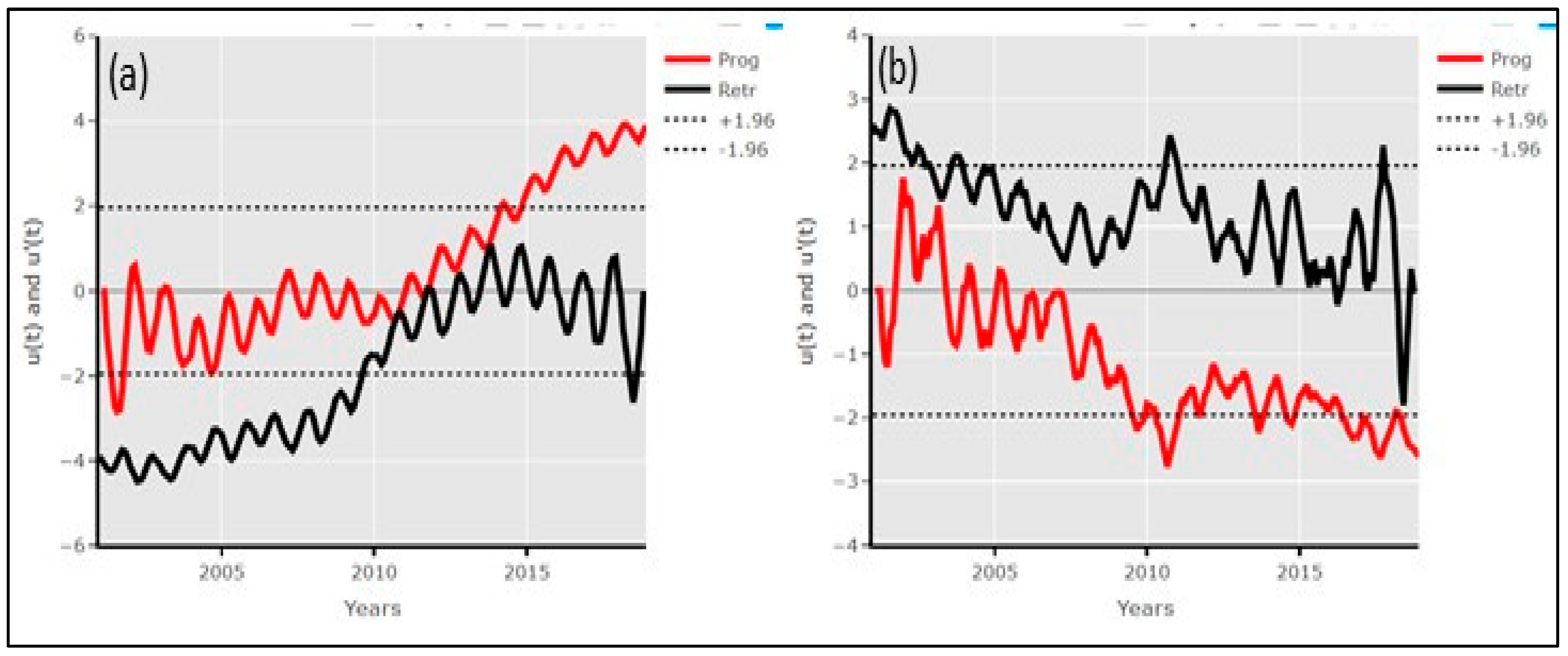
Even though Mann–Kendall is recommended for trend consequence in real time, the MK test has some restrictions preventing it from giving a comprehensive structure of the trend for the entire sequence. There are various underlying forces throughout the trend because of fluctuations over a period investigated; therefore, a specific version of MK test statistics called Sequential Mann–Kendall (SQ-MK) is used for examining each and every individual period [39]. The test is famously known for detecting turning points in the teds and their significance [25,31,39]. SQ-MK test method produces two time sequences, a forward/progressive sequence (u(t)) and a backward/retrograde sequence (u′(t)), and it has the capability to detect predicted potential turning points in trends in lasting series which is achieved by plotting the progressive and retrograde time series in the same graph, if these lines cross each other and diverge beyond the specific threshold (±1.96 in this study), and if there are statistically significant trends [39].

2.9. Multi-Linear Regression (MLR) Model

To further examine the link between ET and other variables, Multi-Linear Regression (MLR) was used. MLR is commonly used to define the connection between single continuous dependent parameters with independent variables [32]. The model number n output is represented by the following formula:
y 1 = β 0   + β 1 x 2 + + β p x i p + ϵ i   where   i = 1 ,   2 ,   3 ,   n
where the dependent variable is ET represented by ( y i ) , and SF, P, NDVI, NDWI, and NDDI are independent parameters represented by x i p . β 0 is the intercept, and the coefficients of x are represented by β 1 , β 2 …… β p . The term ϵ i stands for the error term that is continuously minimised by the model.

2.10. Autoregressive Integrated Moving Average (ARIMA) Model

Autoregressive integrated moving average (ARIMA) was employed in the study. ARIMA is the most utilised modelling technique because of its statistical properties, and it can be used in different ways like pure autoregressive (AR), pure moving average, and combined ARIMA series [40]. Alternatively, the model is also called the Box–Jenkins modelling approach and it is one of the common time-series models because of its flexibility, even though the model is unable to predict the non-linear connections because its model linear correlation structure is presumed among the time values [41]. defined ARIMA as the model that is decomposable into two parts, with the first part being the “Integrated (I) component (d)”, representing the quantity of distinguishing to be achieved on the sequence to make it constant; the second is the ARIMA model sequence that is rendered constant through variation. This model is considered the most effective forecasting tool, and it is widely used in social science and for time series; it also depends on the historical data as well as its past error relations for predicting [42]. Therefore, this study uses ARIMA as one of the two forecasting tools in order to seek the accurate forecasting of ET for the KIS. ARIMA is mathematically defined as follows:
y = θ 0   +   1 y t     1   +   2 y t     2   +     p y t     p   +   ε t     1 ε t     1     2   ε t     2     q ε t
y t and ε t are the actual value and the random error at a given time t . The parameters of the model are   i 1 , 2 , , p and θ j 0 , 1 , 2 , , q . p and q are integers and are normally defined as orders of the model. The random model errors ε t are forecasted to be independently and identically distributed with a mean of zero and a constant variance of σ 2 .

2.11. Artificial Neural Network (ANN) Model

Artificial Neural Networks are a family of artificial intelligence methods capable of forecasting and predicting any time series, including the geophysical time series. These are non-linear data-driven networks that were designed and inspired by the theory of neuroscience [43], hence the name ‘neural’. These are mathematical models based on the capabilities of the human brain to predict and classify problem domains. [44] describe ANN as “the information processing paradigm that is inspired by the way biological nervous systems such as a brain process information”. In essence, Artificial Neural Networks (ANNs) are a semi-parametric regression technique that can estimate any quantifiable function to an unconstrained degree of accuracy [45]. ANNs have been widely accepted for forecasting and estimating in a wide range of scientific domains, including finance, medicine, engineering, and the sciences, in addition to solving an astounding array of issues [46]. Therefore, ANNs are precisely convenient when the links between both input and output variables are distinct [47]. These models have been praised for being helpful in situations when there is an excessive amount of data variety and the relationship between those factors is primarily unclear [47]. This study uses the single hidden-layer feedforward network as one of the methods to forecast. Schultz, Wieland [48] define the single hidden feedforward network as the most utilised models for forecasting and modelling, and for predicting time series. The model has three processing layers which are linked by its acyclic properties and distinguished by its connection between output (yt) and inputs (yt – 1, yt − 2, …, ytp). Schultz, Wieland [48] explained the model mathematical association between the input and output:
y t = α 0 + j = 1 q α j g β 0 j i = 1 p β i j y t 1 + ε t ,
where α j   j = 0 , 1 , 2 , , q and β i j   i = 0 , 1 , 2 , , p ; j = 1 , 2 , , q are the limits which are called the joining weights; p and q are the number of inputs nodes and the number of the hidden nodes, respectively. In designing this type of NNs, the logistic function is mostly utilised as the hidden-layer transfer function that is given by the following:
g x = 1 1 + exp x
The above formula represents a non-linear functional mapping from the past observations ( y t 1 ,   y t 2 , , y t p ) to the future value y t , i.e.,
y t = f y t 1 , y t 2 , , y t p ,   w + ε t
w is a vector of all parameters and f is a function determined by the network structure and connection weights [48].

2.12. ANN Training

A multilayer perceptron (MLP) network type was utilised in this study; hence, it is the common utilised neural network. When given enough information, enough hidden units, and enough time, an MLP may be trained to accurately estimate nearly any function [47].

2.13. Model Statistical Performance Evaluation

There are no set standard norms for assessing a model’s forecasting performance and comparing it to other benchmark models [39]. Therefore, this study used four of the well-known statistical model performance techniques in order to assess the best accurate model to forecast ET over the study area. According to Phesa, Woyessa [1], there are various time-series models used previously to forecast ET; therefore, choosing the best appropriate model considering the conditions is key. Hence, assessing the best suitable model based on forecasting outcomes of ET is key. Four model performance measures are adopted in this study: Root Mean Square Error (RMSE), Mean Absolute Percentage Error (MAPE), Mean Absolute Error (MAE), and the Pearson Correlation Coefficient (R).

2.13.1. Root Mean Square Error (RMSE)

The Root Mean Square Error model performance measure was used to compare the predicted ET values with the actual obtained MODIS ET data.
R M S E = 1 N i = 1 n ( E T e s t i m a t e d i E T r e a l i ) 2
RMSE together with MAE has been employed successfully by [49] to examine the model performance. These two model performance evaluation measures were further tested by [50] and results showed that RMSE was not a perfect indicator of model performance; however, [49] found contradicting results, even though they also suggested that not using the absolute value was the key advantage of RMSE.

2.13.2. Mean Absolute Percentage Error (MAPE)

The MAPE is the second model performance measure employed in this study. MAPE has been widely used as a model performance measure because of its intuitive proportion judgement or error. This measure is commonly adopted over other models when the amount to predict is known and higher than zero [51].
M A P E = 1 N i = 1 n E T e s t i m a t e d i E T r e a l P E T r e a l i × 100 %
According to [52], MAPE “is calculated using the absolute error in each period divided by the observed values that are evident for the period, then average those fixed percentages”. It is also used to calculate the borderline error in a predicted least squares method of data analysis and it shows the quantity or error [51].

2.13.3. Mean Absolute Error

Mean Absolute Error (MAE) is the third model performance measure used in this study. It was another measure used to assess the accuracy of the three selected models in this study. MAE is calculated from an average error and it is used frequently to evaluate vector-to-vector regression models.
M A E = 1 n i = 1 N ET estimated i ET real i
A study by [53] used MAE, and the model outsmarted other models like the RMSE. This measure is calculated by summing the absolute values of the error to obtain the sum error, and then dividing the total error by a generic method suggested by Willmott and Matsuura (2005) [52].

2.13.4. Pearson’s Correlation Coefficient

Ref. [54] defines correlation coefficient as a method for statistically examining a likely, two-way, linear relationship between two continuous variables. Where X i 0   and   X i p are the individual data points for the two variables, X 0 ¯ and X p ¯ are the means of the two variables and n is the number of data points [55].
R = 1 = 1 n ( X i 0 X 0 ) ¯ X i p X p ¯ i = 1 n ( X i 0 X 0 ) ¯ 2   i = 1 n ( R i p X p ) ¯ 2
The model performance is used to measure the reputed strength of the linear relationship between the tested variables. A correlation coefficient value of zero indicates that there is no linear association between the two variables. A value between +1 and −1 indicates a perfect correlation, the strength of which is indicated anywhere between +1 and −1. A positive value indicates a direct relationship between two variables and a negative value indicates that there is an inverse relationship between two variables [54].

3. Results and Discussions

3.1. The Breaks for Additive Seasonal and Trend (BFAST) Analysis

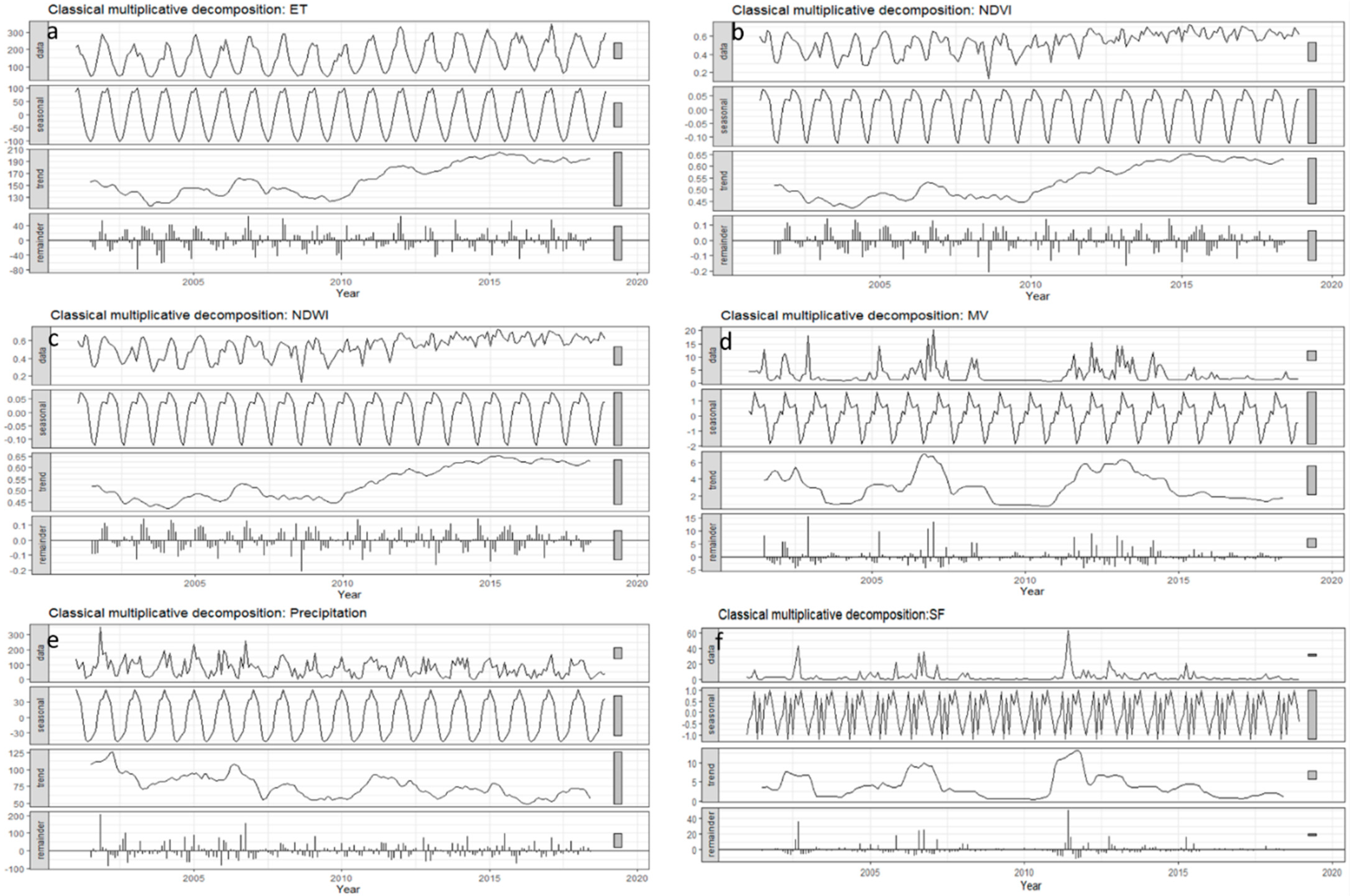
The time series of the obtained parameters was constructed in order to evaluate the variability in these variables. Figure 2a–f show the temporal variability of ET, NDVI, NDWI, Dam MV, P, and SF. The Breaks for Additive Seasonal and Trend (BFAST) technique is commonly utilised to assess the difference in time series and incorporate the breakdown of time series to trend components, residual components, and seasonal components. This method assists in sensing and describing the unforeseen differences within the trend and its seasonal components [25]. The first panel in Figure 2a–f shows the original obtained time series from the study site, followed by the trend on which the analysis is based.
Figure 2a shows that the annual ET decreased during the 2001 to 2003 period, reaching zero. From 2003, it is evident that there was an increase in ET, which started increasing upward until 2007. The period of 2007 to 2010 shows another decline in ET and, contrary to that, an upward trend showing an increase from 2010 to 2018. This agrees with the fact that, from the year 2010, to date, there have been irrigation activities going on at the KIS. Figure 2b shows an almost similar trend to the ET trend; from 2001 to 2003, it is evident that greenness at the KIS declined; however, from 2003 to 2007, the water content started increasing, leading to an NDVI increase. From 2007, the trend is parallel to the ET trend where the vegetation greenness declines up to the year 2010. From the period of 2010 to 2018, the NDVI trend shows an increase with an upward trend. This evident increase from 2010 also indicates the irrigation activities happening at the study site are similar to ET increase.
Equally, the NDWI trend indicated by Figure 2c matches the NDVI trend over the 18-year (2001–2018) period. This shows an improvement in the water over the study area. Figure 2d shows the temporal variability of the Sandile Dam monthly volume over the 18-year (2001–2018) period. During 2001, the monthly volume at the Sandile Dam shows a decline, with dam levels reaching almost zero. It is evident that, during 2004, the trend started increasing with a spike in 2007, and then the monthly volume decreased from 2009 until 2011, with the Sandile Dam reaching the lowest levels, which started to improve from 2011 to 2013, and, from then, there has been a significant decrease in this dam’s levels. Likewise, precipitation over the study area is shown in Figure 2e; this figure shows the P trend constantly decreasing from 2001 to 2010, and then, from the period of 2010 to 2018, unstable precipitation is noted over the study area. This verifies the decrease in the Sandile Dam monthly volumes over this period. Lastly, Keiskammahoek River, which is the feeder river to the Sandile Dam, is shown in Figure 2f. This figure shows a decreasing trend from the period of 2001 to 2003; from 2003, the figure shows an improvement in streamflow volumes with an upward trend until 2007. However, from 2007 to 2011, the streamflow volume started decreasing again with the lowest streamflow volumes during 2011. From 2011 to 2012, there is a spike in the river trend, and then, from 2012, the streamflow decreases continuously until the year 2018. The constant trend noted for ET, NDVI, and NDWI as indicated by Figure 2a–c clearly shows that there is a string connection between these variables. These results agree with the [56] study which proved that healthy plants transpire more water, which lead to higher ET values. Equally, Ref. [57] reported that higher ET could be due to water availability. This shows that, mostly from 2010 to 2018, there were irrigation activities in the study area. Conversely, SF, MV, and P decline compared to other variables; this indicates opposing results compared to the NDWI, NDVI, and ET rising trend.

3.2. Wavelength Analysis Results

Figure 3 shows the monthly mean ET (a) and P (b) normalised wavelet power spectra for the period of 2001 to 2018. The “u”-shaped solid line in the figure shows the cone of influence (COI), defining the area of the spectrum that must be deliberated in examination. The COI represents the region in which edge effects transpire. The 95% confidence level is represented by a black line which is significant for the region. The blue colour presents the lowest wavelet power and the red colour represents the regions which have more wavelet power. The period in months is shown by the vertical axis, and the horizontal axis represents the time in years [31].
A strong wavelet power spectra over 12 months is noted from the years 2001–2018, However, in the wavelet transforms of the P, it is apparent that the 12-months power spectrum was strong during the period of 2001 to 2015 and the wavelet power spectra were very weak during 2015 to 2018. The weak seasonality power spectrum might have been because of the decrease in P that occurred, with P reaching almost 0 mm in 2015. The decrease in P could be led by strong El Niño events that occurred during the period from late 2014 to 2016 [32]. The P power spectra also experience several shorter periods of significant power, primarily during 2002 and 2006.

3.3. Wavelet Coherence Results

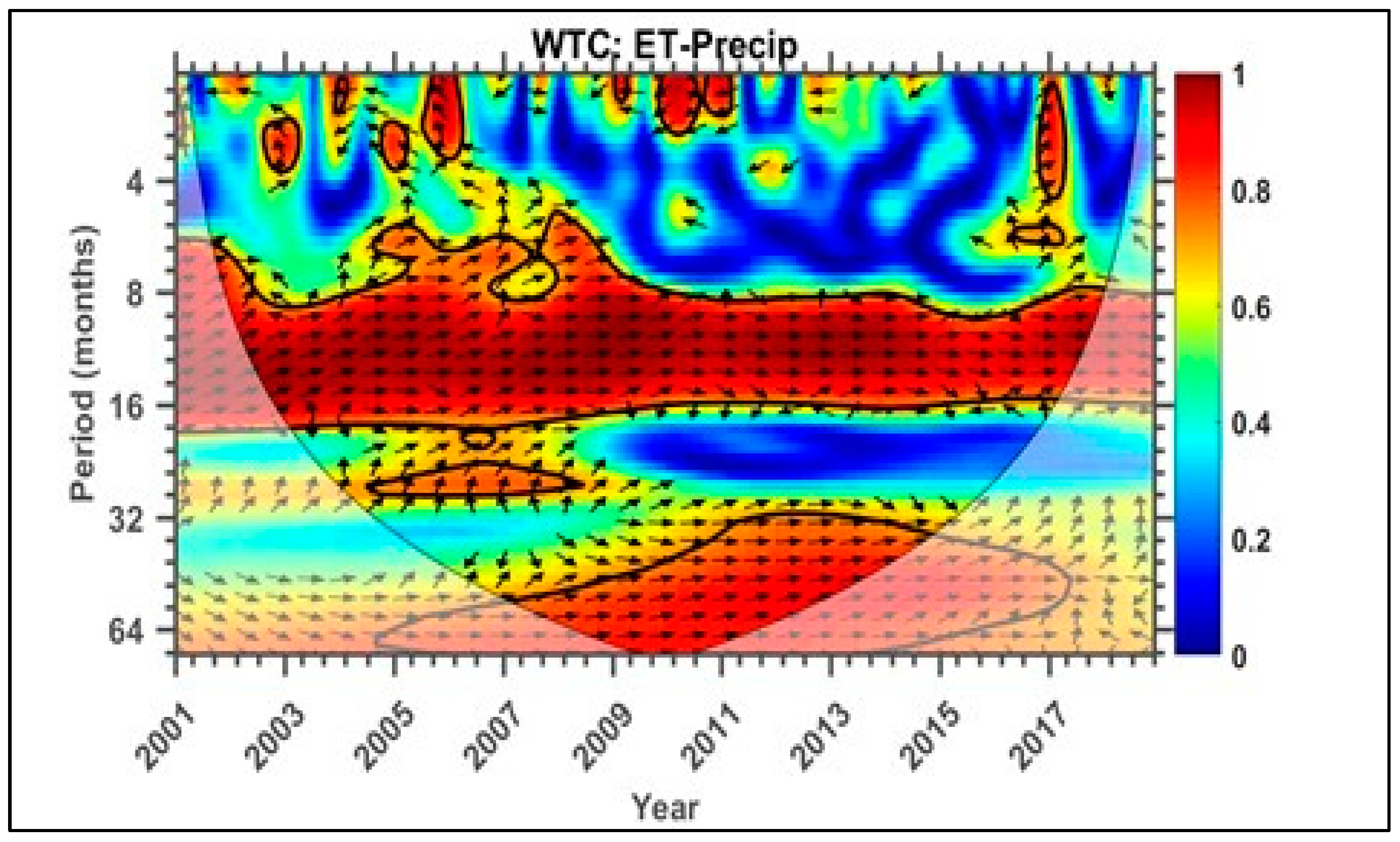
Figure 4 shows the cross-wavelet power spectra for ET and precipitation with the phase connection indicated by arrows. The area where two cross-wavelet factors are in phase is indicated by arrows pointing to the right, and the anti-phase is indicated by arrows pointing to the left, and the ET lagging or leading is indicated by arrows pointing downwards or upwards correspondingly [58]. The black solid line indicates the cone of influence (COI), the edge effects develop significant frequency scales, and the line also indicates the significant areas with a 95% confidence level.
In general, it is confirmed that there is a possible strong and significant in-phase relationship between ET and precipitation during 2001 to 2018, indicated in the period bands of 8 months to 16 months, with arrows pointing right (phase). It is noted that, in band 1 to 5, there is an anti-phase connection between P and ET, and this happened from the years 2003 to 2006 and from 2009 to 2010. However, in the year 2017, changes start to be noted where the ET leads P, with arrows pointing up. During the period of 2001 to 2009, it is noted that ET led P, shown by upward arrows, then rotating to the right in the time period bands. However, in the period bands of 34 to 64 months, with arrows pointing downward showing lagging, and arrows turning right showing a phase relationship from 2001, reaching a 95% confidence level during 2007 to 2015, indicating a very strong phase relationship with precipitation leading ET. During the period of 2015 to 2018, it is evident that there are some arrows pointing right, showing a phase relationship between the two variables, but, there, ET seems to be leading, with arrows pointing up.

3.4. Correlation Statistics

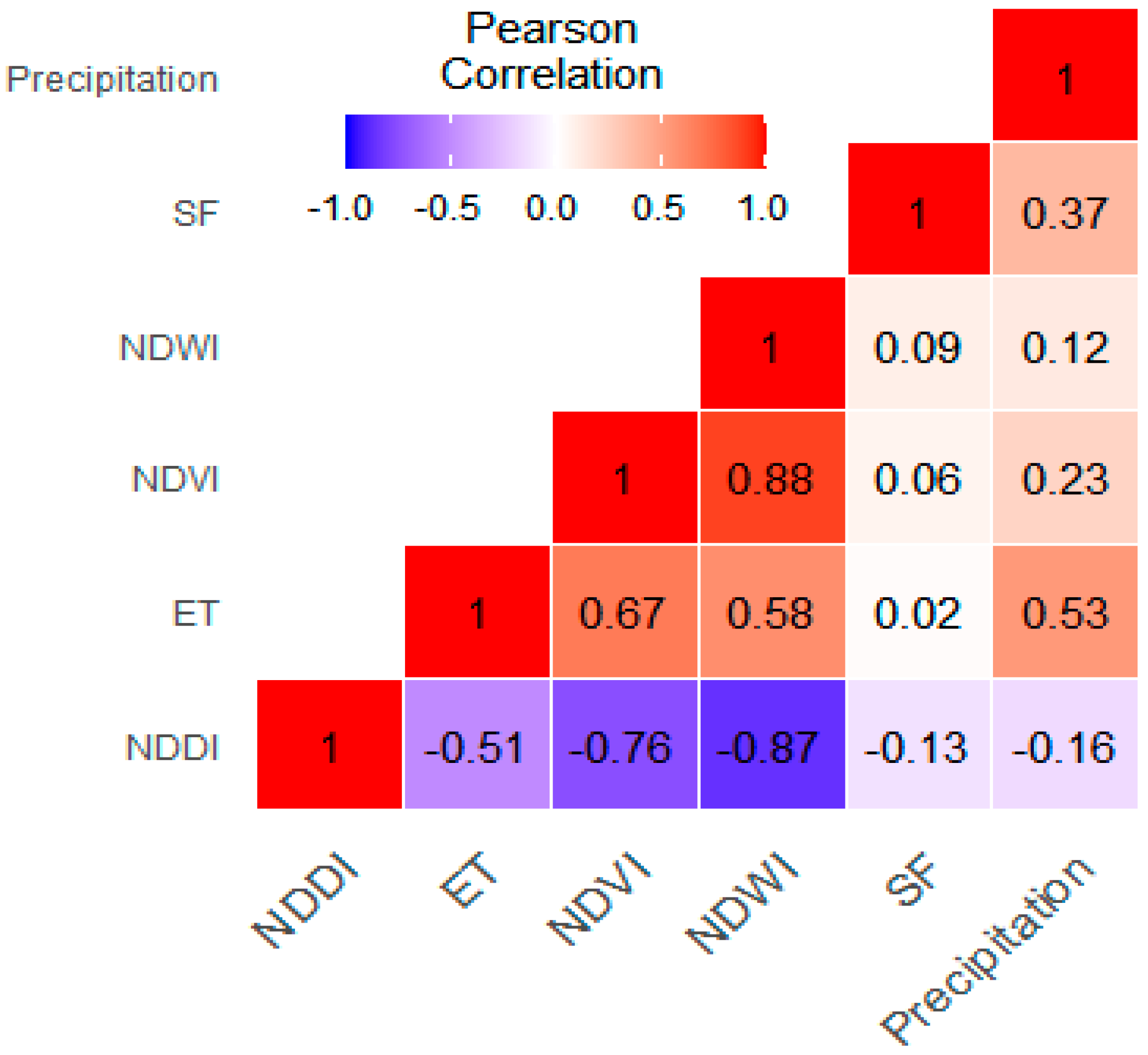
The correlation between ET and the other parameters was carried out in order to understand the relationship between these variables. Figure 5 shows a heat map with the linear correlation between all the variables.
Figure 5 strongly suggests a negative correlation between ET and NDDI (−0.51), signified by the ET correlation relationship with SF (r = 0.02). However, in the above figure, it is also evident that ET has a strong relationship with other parameters tested with NDVI (r = 0.67), NDWI (r = 0.58), and precipitation (r = 0.53). This negative correlation between NDDI, which is the drought index, simply justifies that there was no severe drought at the study site with P (−0.16), SF (−0.130), NDWI (−0.87), NDVI (−0.76), and ET (−0.51). NDDI is the best index that could be used to assess drought as it includes both the water content and the vegetation, which, henceforward, should be assessed in a dry season/dry surface in order to obtain the strong correlation [59]. This negative correlation simply justifies the irrigation activities that took place from the years 2010–2018. The strong correlation between ET, NDWI (0.58), and NDVI (0.67) shows that there was no water shortage at the KIS and, equally, vegetation was not under stress. This contradicts the results of the Theil–Sen estimator which shows a significant decrease in precipitation with p < 0.001. The NDVI results and P are interesting as they agree with Palacios-Orueta, Khanna [60] where the NDVI flow precipitation results in irrigated regions. Even though there is a correlation between NDVI and P, it is not strong, which is contrary to the results found by Ding, Zhang [61], who found a similar correlation between NDVI and precipitation. Other studies like that of Tavazohi and Nadoushan [29] showed that a decrease in available-supply water reserves like precipitation gives negative correlation between the NDWI and other parameters. According to Aksoy, Gorucu [62], drought is triggered by a decrease in precipitation and an increase in evapotranspiration, and, based on the assessed time-series data, a decrease in precipitation, streamflow, and dam levels indicates some signs of drought in this region.

3.5. Theil–Sen Plot

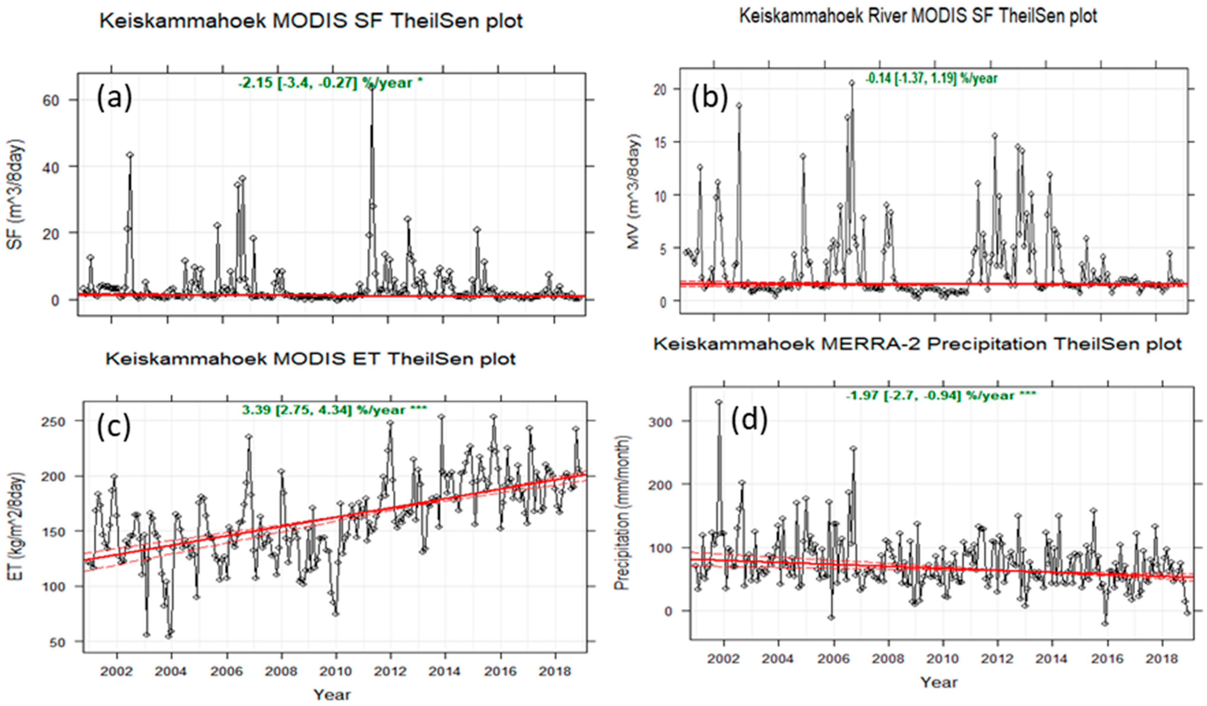
Figure 6 depicts the time evolution of the de-seasonalised monthly mean for the SF (a), MV (b), ET (c), and P (d) time series over 18 years (2001–2018). There are 216 trend lines used by the Theil–Sen function for all the variables. The solid line indicates the estimate and the dashed red line shows the 95% confidence intervals of the trend based on the parameters. The complete trend shows the following: for the streamflow (a), −2.15 m3/year at confidence levels of −3.4 to 0.27 m3/year; −0.14 m3/year for the monthly volumes of the Sandile Dam (b) at a confidence level of −1.37 to 1.19 m3/year; for ET (c), 3.39, at a confidence level of 2.75 to 4.34 km/m2/year (a); and −1.97 mm/year at a 95% confidence level of −2.7 to −0.94 mm/year for precipitation (d). The p-value governs the symbols used and that is represented by p < 0.001 = ***, p < 0.01 = **, p < 0.05 = *, and p < 0.1 = +. The three stars show an extremely statistically significant trend estimate, but the plus sign indicates a trend prediction that is not statistically significant [63].
For the SF shown in Figure 6a, the Theil–Sen trend estimation shows a significantly decreasing downward trend with a p-value of −2.15 m3/s. This indicates a decrease in the SF of Keiskamahoek River which is the supply river to the KIS. The Sandile Dam Theil–Sen estimator, a lower supply dam to the KIS, equally shows a downward trend of −0.14 m3/year. In terms of the trend being significant, and according to the Theil–Sen function, this shows a less significant decrease in dam levels over the study period with a p-value of −0.14 m3/year. The figure further shows the annual evolution of ET, displaying a positive slope, which matches with the increasing trend shown by Figure 6c at 3.39 kg/m2 per year, and this upsurge is strongly significant with p < 0.001. It is further noted that Figure 6d shows a downward slope for P for the years 2001–2018, confirmed at −1.97 mm/year with a p-value of 0.001, showing a significant decrease in precipitation over this value. According to Wu, Chen [64], the decrease in precipitation is highly affected by hydrological drought and this further affects the streamflow. These results are also interesting as they agree with Speer, Leslie [65], who found that the decrease in river streamflow is directly related to the decrease in precipitation.

3.6. Mann–Kendall Test (MK)

To investigate the significance, the MK test was used in this study. Table 1 indicates a Mann–Kendall test model for all seven variables that are also tested by this study. According to Xulu, Peerbhay [25], the MK trend test model is employed in order to measure the trend’s significance, with a z-score between −1.96 and +1.96 showing the non-significance of the trend, and, if the variables fall outside of the range, the trend is taken as being significant. For this study, this trend test was employed with ±1.95 boundary lines which specify 95% confidence levels.
The indicated z-score for ET in Table 1 shows a z-score value equal to +3.898, a value far greater than +1.96, and this indicates a significant positive trend with a cut-off line at the 95% confidence level. This signifies that, over the 18-year (2001–2018) period, there has been an increase in ET at the KIS. Contrary to this, it is noted that the z-score for precipitation is equal to −2.6134, indicating a significant decrease in precipitation during the study period of 18 years (2001–2018). This shows a significant decrease in precipitation variability over the 18-year period. Equally, there is a noted decrease in SF for the supply river Keiskammahoek River with a z-score equal to −1.7508.
Equivalent to that, the Sandile Dam volumes z-score is equal to +0,60747, showing a non-significant increase over the study period. It is further noted that there was a significant increase in NDVI over the 18-year period with a z-score reaching +8.3291, which agrees with the strong significant increase in NDWI over this period, with a z-score equal to +10.021. It is noted that the NDDI decreases over the study period with a z-score equal to −9.8859, showing a strong decrease in this value. The NDDI has, in the past, been used as a critical index to assess drought because of its ability to include both the vegetation and water conditions [66]. The significant decrease in NDDI values as indicated by the z-score agrees with Mujiyo and Komariah [67], who state that “higher values of NDDI indicate drought and lower values indicate that the arear have some moisture, therefore not experiencing drought”.

3.7. Sequential Mann–Kendall (SQ-MK)

Further to the Mann–Kendall Test, the Sequential Mann–Kendall (SQ-MK) is used to show the trend and its significance to ET and precipitation. This is carried out in order to see the detection points of the trend and its points. Figure 7 depicts the sequential statistics value of forward/progressive (Prog) u(t) (red solid line) and backwards/retrograde (Retr) u(t) (solid black line), calculated using the SQ-MK for the ET time series extracted from the KIS. In general, there is an upward trend evident in the SQ-MK parameters from the beginning of the time series.
The SQ-MK test for ET presented in Figure 7a shows the change detection point is from the period between 2012 and 2014. After the change detection points during this period, the progressive time series increases until it reaches a significant level during 2015. The time series of the progressive statistic reaches z-score values which are approximately equal to 4 towards the end of the time series. This indicates that there has been an increase in the ET rate at the study site that started just after the year 2010. This increase is presumed to be associated with a continual increase in average surface temperatures as well as the intense El Niño events that affected the eastern part of South Africa in recent years [32].
Furthermore, Figure 7b shows SQ-MK test values of forward/progressive (Prog) u(t) (solid line) and retrograde (Retr) u’(t) (black solid line) for precipitation data from the period of 2001 to 2018. Based on this figure, from 2010, there has been a decrease in the trend, reaching a significant level just after 2010, as indicated by the progressive statistic. From 2010, it is noted that a further decrease which is significant is noted, fluctuating between –1.96 and below −1.96, indicating various incidents of negative and significant values on the trend. Parry and Carter [68] suggested that both ET and precipitation have a relationship and a decrease in precipitation directly increases ET. The study indicates a decrease shown by a downward trend shown by Prog during the period of 2016 to 2018. From 2001 to September 2002, the figure shows that precipitation decreased with a significant downward trend, with (Tetr) decreasing from 2.613 to 2.099. Prog values also show a non-significant decrease in precipitation from the year 2001 to May 2010, but this decrease became significant and reached a maximum value of −2.77 in September 2010. Both Retr and Prog start decreasing until 2018, even though some insignificant trends are evident in both Retr and Prog values. It can be concluded that the SQ-MK test for ET data shows ET at the KIS is subject to an increasing trend with no significant decrease, and the effect of irrigation activities on the study site led to the increase in ET becoming a significant trend. Parallel to that, precipitation is subjected to a decrease, even though, most of the time, both the Retr and Prog values are not significant. The last results indicate a significant decrease, with a negative Prog of −2.613.

3.8. Multi-Linear Regression (MLR) Analysis

To further interpret the relationship between ET and other variables, the MLR model is used in the study. The model is well-known for its capability to define relationships between a single continuous dependent variable and two or more supplementary independent variables [32].
The MLR analysis is shown in Table 2, encompassing ET, SF, P, NDVI, NDWI, and NDDI. ET and related variables influencing ET were examined to determine their degree of influence on ET at the KIS. Based on these results, it is shown that ET has a string connection between ET and SF, precipitation, and NDVI with their p-values of 2.32 × 10⁻⁶ for SF, 2.32 × 10⁻⁶ for precipitation, and 2 × 10⁻¹⁶ for NDVI. This correlation demonstrates a statistically significant relationship between ET and the three variables since their ρ-values are less than 0.05. However, the statistical relationship between ET and NDDI was found not to be very significant with a p-value of 0.0208, which is greater than 0.05, but it is still significant. It is also indicated in Table 2 that the relationship between ET and NDWI is statistically insignificant with a p-value of 0.5441, which is greater than 0.05.

3.9. ARIMA Training and Validation

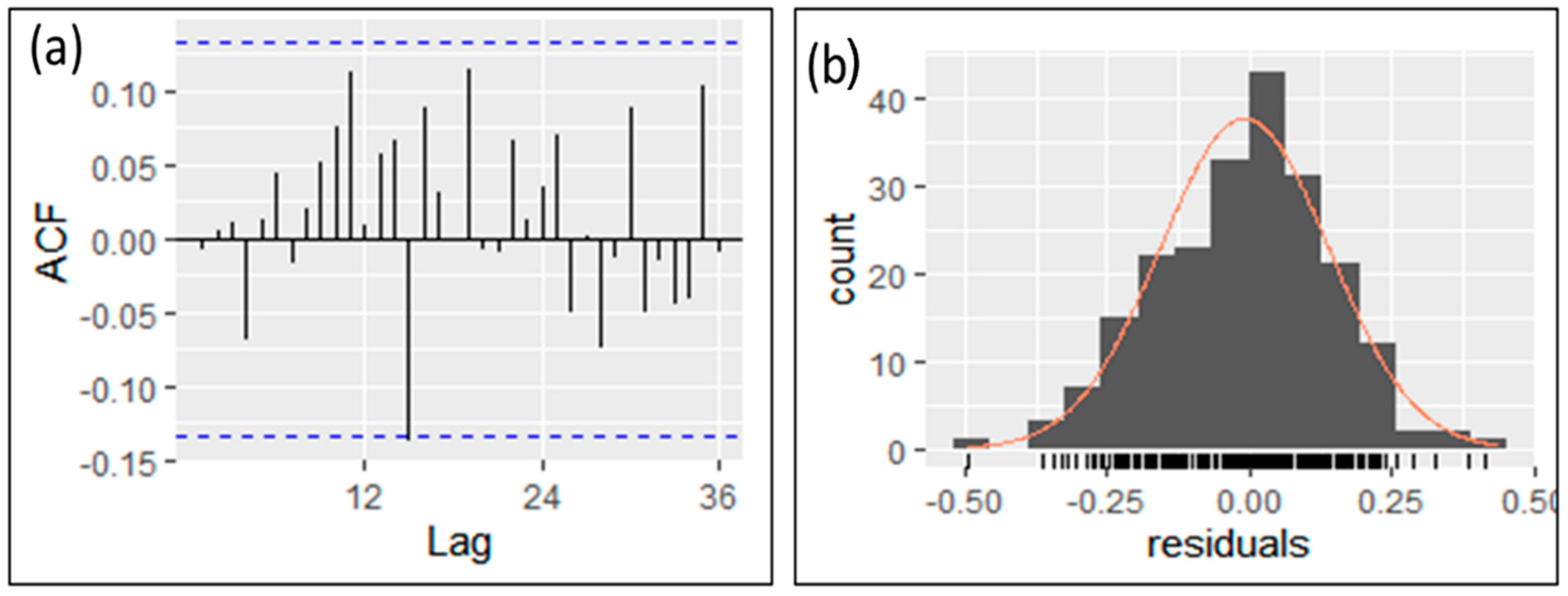
The ARIMA model was trained to ensure that the model will fit with the data. The 18-year (2001 to 2018) data were fitted on AUTOARIM using “R” and a portmanteau test called Ljung–Box was carried out to test the excellence of the time-series model. Ghauri, Ahmed [69] suggested that, when the test is used, and should the significant auto-correlation not be found in the model residuals, the model is considered to be perfect. If the values of the correlation of residuals for various time lags is not significantly different from zero, the model is then considered to be adequate for use in prediction. The following is the Akaike’s Information Criteria (AIC) graph which shows that there are significant correlations because all the bars do not exceed the dotted line indicating the 95% confidence levels, and, according to [70], this further suggested if the residue is random. The best-fitting model used by this study was ARIMA(1,0,0).
Figure 8a,b depict the residual values as evenly dispersed. Reza and Debnath [71] suggested that the normal distribution of residual values shows that the selected ARIMA model is free of overfitting.

3.10. ARIMA Forecasting

Figure 9 depicts the forecasted results of ET using ARIMA. Figure 9a shows the time-series data from 2001 to 2016 indicated by the dark grey and light grey shadings, showing the 80% to 95% confidence levels of the forecasted results. The remaining three years forecasted using ARIMA from the years 2015 to 2018 are indicated by the blue line on a dark grey shadow. Figure 9b shows the correlation coefficient between the forecasted data and the obtained data from the KIS. This scatter plot showing black dots on top of the line shows the obtained data versus the forecasted results and the R = 0.94. This indicates a very strong correlation between the forecasted results and the original results. Additionally the scatter plot blue line represent the summary of the overall trend of the data points showing the best fit of the dataset.
The results shown in Figure 9 agrees with [72] as they have proven that ARIMA is one of the best models for the forecast of evapotranspiration. Furthermore, this study proved that ARIMA models are superior to machine-learning models due to their accurate forecasting capability and less complexity. Moreover, the 0.94 correlation achieved by ARIMA models indicates a very strong linear connection between the original data and the forecasted ET data. According to Schober, Boer [73], the closer the correlation is to 1, the more accurate the model is for the increase in one variable and shows a strong relationship to the increase in the other variable. The robustness of an ARIMA model refers to its ability to perform well in various conditions, especially when there are challenges like non-stationarity, seasonality, or outliers in the data.

3.11. ANN Modelling

The Artificial Neural Network (ANN) is the second model used in this study. The second model is used in order to assess the best alternative models that could assist in forecasting ET at the KIS. Figure 10a shows the 15-year (2001 to 2015) data indicated by the blackline. The remaining three years (2015 to 2018) show the forecasted ET. Furthermore, Figure 10b shows the scatter plot, showing two variables indicated by the black dots on top and underneath the blue diagonal line. According to Sapankevych and Sankar [74], the ANN models are particularly well-suited for the prediction of the non-linear components of time-series data. This capability makes them a powerful tool for modelling complex and dynamic systems where traditional linear models may fall short.
Likewise, the ANN models prove to be one of the effective models to forecast ET for the KIS. The correlation indicated by R = 0.86 shows a stronger correlation between the original ET data and the forecasted ET values. These results agrees with the results of Zhang [75], which proves that the ANN could forecast the time series effectively. Additionally, a correlation of 0.86 indicated by the scatter plot suggests that the ANN model is able to capture the underlying patterns in the data reasonably well. The predictions are closely aligned with the actual outcomes, indicating that the model is effective in making forecasts.

3.12. Model Performance Comparisons

The four statistical model performance evaluators were applied as shown in Table 3. According to Rahman and Devanbu [76], evaluating the performance of a statistical model involves using various metrics and functions to quantify how well the model’s forecast aligns with the actual data. Equally, Ref. [77] suggested that the lower the model performance, the better the forecasting model. Based on these results, it is clear that the ARIMA model performs better compared to the ANN models. The lower ARIMA values of the RMSE = 37.58 are lower than the ANN values of the RMSE = 44.18; the ARIMA values of the MAE = 32.37 are lower than the ANN values of the MAE = 35.88; the ARIMA values of the MAPE = 17.26 are lower than the ANN values of the MAPE = 24.35; and the correlation values of the ARIMA with the R = 0.94 shows a higher accuracy compared to the ANN with the R = 0.86. These model performance indicators proved that, in the two selected models in this study, the ARIMA models outperform the ANN models.
Likewise, these results agrees with the results of Fashae, Olusola [78], where the ARIMA forecasting models achieved better results compared to the ANN forecasting models. These results are interesting as they are contrary to various studies [79,80,81] which proved that the ANN performs better than ARIMA. Therefore, ARIMA models have a full potential to forecast ET for the Keiskammahoek Irrigation Scheme as an alternative model to the famous old ET forecasting tools. Even though the selected ARIMA(1,0,0) model performs well and is an easily interpretable model that works well under certain conditions, the model robustness can be questionable because of the non-stationarity, outliers, and non-linearity of the time series as the model only deals with a linear part of the time series [82]. According to [83], the selected model by auto-ARIMA, ARIMA(1,0,0) is a linear model, which assumes a linear relationship between current and past observations. Therefore, even though these results are accurate and outperform the ANN, there are areas of improvements in terms of ensuring that the model is robust enough to work across the variety of conditions which may include data with noise, outliers, and changes in the structure of the data. Because of the inability for ARIMA to handle non-linear time series, the ANN with the ability to deal with a non-linear dataset, as employed by this study, performed poorly compared to ARIMA. This poor performance according to [83] may be caused by the nature of the dataset and the different approach with which each model deals with forecasting. Additionally, ANNs require a large amount of data to train the model effectively; hence, small datasets lead to model overfitting and fitting poorly, which also leads to poor forecasting. Nevertheless, the accurate forecasting of ET for the KIS will play a crucial role in managing water resources. The precise forecasting and estimation of ET have a direct impact on the aspects of optimum water management, particularly for irrigation management.

4. Conclusions

The study focused on assessing the best-performing model that could forecast evapotranspiration (ET) in a water-scarce irrigation scheme in the Eastern Cape Province of South Africa. The irrigation schemes in the Eastern Cape suffer greatly from water scarcity as a result of periodic droughts. Hence, the province has been declared as water-stressed. This led to water managers struggling to plan effectively in order to keep the water resources available for the livelihood of the irrigation scheme. The teleconnection evaluation between the satellite-derived ET with NDVI, NDWI, NDVI, and P is used to determine the significance and the dynamics within the ET and other parameters. In general, the results of the Mann–Kendall (MK) test indicate a significant upward trend of ET (z-score = +3.898), which is greater than +1.96, an indication of the trend’s significance. In contrast, there is a significant decrease in the other variables, such as precipitation (z-score of −2.6134) and NDDI (z-score = −9.886), over the 18-year period. The results of the-Multi Linear Regression proved that there is a statistically significant relationship between ET (p-value < 2 × 10⁻¹⁶), NDVI (p-value of 7.89 × 10⁻¹¹), SF (p-value of 2.32 × 10⁻⁶), P (p-value < 2 × 10⁻¹⁶), and NDDI (with p-value of 0.0208), respectively. Since the p-values are less than 0.05, this implies that ET strongly depends on the precipitation, vegetation health, and response of the vegetation to drought conditions at the study area. Moreover, the consistent decrease in the other variables such as streamflow and the monthly volumes of the Sandile Dam is an indication of drought in the study area. Furthermore, the study forecasted ET using the two famous machine-learning forecasting tools, the ARIMA and ANN models. The forecasting results indicate that the ARIMA models could be used as an alternative robust model to forecast ET at the irrigation scheme over the ANN with the RMSE for the ARIMA = 37.58, over the ANN = 44.18; the MAE for the ARIMA = 32.37, over the ANN = 35.88; the MAPE for the ARIMA = 17.26, over the ANN = 24.26; and for the R ARIMA = 0.94 and for the ANN = 0.86.

Author Contributions

Conceptualisation, M.P. and N.M.; methodology, M.P. and N.M.; software, N.M. and M.P.; validation, M.P.; formal analysis, M.P. and N.M.; investigation, M.P.; resources, M.P. and N.M.; data curation, M.P. and N.M.; writing—original draft preparation, M.P.; writing—review and editing, N.M. and A.I. All authors have read and agreed to the published version of the manuscript.

Funding

The authors are grateful to the Faculty of Engineering, Built Environment & Information Technology (FEBEIT), and Walter Sisulu University (WSU) for financial support.

Data Availability Statement

The dataset used in this manuscript is available from the corresponding author upon reasonable request.

Acknowledgments

The authors would like to thank all personnel involved in the development of the Google Earth Engine system and climate engine. We also thank the providers of the important public dataset in the Google Earth Engine, in particular, NASA, USGS, NOAA, EC/ESA, and the MERRA-2 model developers.

Conflicts of Interest

The authors Mbulelo Phesa, Nkanyiso Mbatha, and Akinola Ikudayisi declare no conflicts of interest. Furthermore, the funders had no role in the design of the study; in the collection, analyses, or interpretation of the data; in the writing of the manuscript; or in the decision to publish the results.

References

  1. Adebiyi, A.A.; Adewumi, A.O.; Ayo, C.K. Comparison of ARIMA and Artificial Neural Networks Models for Stock Price Prediction. J. Appl. Math. 2015, 2015, 614342. [Google Scholar] [CrossRef]
  2. Aghelpour, P.; Norooz-Valashedi, R. Predicting daily reference evapotranspiration rates in a humid region, comparison of seven various data-based predictor models. Stoch. Environ. Res. Risk Assess. 2022, 36, 4133–4155. [Google Scholar] [CrossRef]
  3. Aksoy, S.; Gorucu, O.; Sertel, E. Drought Monitoring using MODIS derived indices and Google Earth Engine Platform. In Proceedings of the 2019 8th International Confrence on Agro geoinformatics, Istanbul, Turkey, 16–19 July 2019. [Google Scholar]
  4. Albalawi, S. River Water Level Forecasting with Adaptive ARIMA and Extreme Learning Machine Models. Doctoral Dissertation, Flinders University, College of Science and Engineering, Adelaide, Australia, 2023. [Google Scholar]
  5. Aouissi, J.; Benabdallah, S.; Chabaâne, Z.L.; Cudennec, C. Evaluation of potential evapotranspiration assessment methods for hydrological modelling with SWAT—Application in data-scarce rural Tunisia. Agric. Water Manag. 2016, 174, 39–51. [Google Scholar] [CrossRef]
  6. Archer, E.; Du Toit, J.; Engelbrecht, C.; Hoffman, M.T.; Landman, W.; Malherbe, J.; Stern, M. The 2015-19 multi year drought in the Eastern Cape, South Africa: It’s evolution and impacts on agriculture. J. Arid Environ. 2022, 196, 104630. [Google Scholar] [CrossRef]
  7. Bencherif, H.; Toihir, A.M.; Mbatha, N.; Sivakumar, V.; Du Preez, D.J.; Bègue, N.; Coetzee, G. Ozone variability and trend estimates from 20-years of ground-based and satellite observations at Irene Station, South Africa. Atmosphere 2020, 11, 1216. [Google Scholar] [CrossRef]
  8. Carter, C.; Liang, S. Evaluation of ten machine learning methods for estimating terrestrial evapotranspiration from remote sensing. Int. J. Appl. Earth Obs. Geoinf. 2019, 78, 86–92. [Google Scholar] [CrossRef]
  9. Chai, T.; Draxler, R.R. Root mean square error (RMSE) or mean absolute error (MAE)?–Arguments against avoiding RMSE in the literature. Geosci. Model Dev. 2014, 7, 1247–1250. [Google Scholar] [CrossRef]
  10. Chen, L.; Lai, X. Comparison between ARIMA and ANN models used in short-term wind speed forecasting. In Proceedings of the 2011 Asia-Pacific Power and Energy Engineering Conference, Wuhan, China, 25–28 March 2011; pp. 1–4. [Google Scholar]
  11. Cunha, A.; Alvalá, R.C.; Nobre, C.A.; Carvalho, M.A. Monitoring vegetative drought dynamics in the Brazilian semiarid region. Agric. For. Meteorol. 2015, 214, 494–505. [Google Scholar] [CrossRef]
  12. Dang, X.; Peng, H.; Wang, X.; Zhang, H. Theil-sen estimators in a multiple linear regression model. Olemiss Edu 2008, 2, 1–30. [Google Scholar]
  13. de Andrade, B.C.C.; de Andrade Pinto, E.J.; Ruhoff, A.; Senay, G.B. Remote sensing-based actual evapotranspiration assessment in a data-scarce area of Brazil: A case study of the Urucuia Aquifer System. Int. J. Appl. Earth Obs. Geoinf. 2021, 98, 102298. [Google Scholar] [CrossRef]
  14. De Myttenaere, A.; Golden, B.; Le Grand, B.; Rossi, F. Mean absolute percentage error for regression models. Neurocomputing 2016, 192, 38–48. [Google Scholar] [CrossRef]
  15. Dias, S.H.B.; Filgueiras, R.; Fernandes Filho, E.I.; Arcanjo, G.S.; Silva, G.H.d.; Mantovani, E.C.; Cunha, F.F.d. Reference evapotranspiration of Brazil modeled with machine learning techniques and remote sensing. PLoS ONE 2021, 16, e0245834. [Google Scholar] [CrossRef] [PubMed]
  16. Dile, Y.T.; Ayana, E.K.; Worqlul, A.W.; Xie, H.; Srinivasan, R.; Lefore, N.; You, L.; Clarke, N. Evaluating satellite-based evapotranspiration estimates for hydrological applications in data-scarce regions: A case in Ethiopia. Sci. Total Environ. 2020, 743, 140702. [Google Scholar] [CrossRef] [PubMed]
  17. Ding, M.; Zhang, Y.; Liu, L.; Zhang, W.; Wang, Z.; Bai, W. The relationship between NDVI and precipitation on the Tibetan Plateau. J. Geogr. Sci. 2007, 17, 259–268. [Google Scholar] [CrossRef]
  18. Dinpashoh, Y.; Jhajharia, D.; Fakheri-Fard, A.; Singh, V.P.; Kahya, E. Trends in reference crop evapotranspiration over Iran. J. Hydrol. 2011, 399, 422–433. [Google Scholar] [CrossRef]
  19. Er-Raki, S.; Chehbouni, A.; Khabba, S.; Simonneaux, V.; Jarlan, L.; Ouldbba, A.; Rodriguez, J.; Allen, R. Assessment of reference evapotranspiration methods in semi-arid regions: Can weather forecast data be used as alternate of ground meteorological parameters? J. Arid Environ. 2010, 74, 1587–1596. [Google Scholar] [CrossRef]
  20. Fang, W.; Huang, S.; Huang, Q.; Huang, G.; Meng, E.; Luan, J. Reference evapotranspiration forecasting based on local meteorological and global climate information screened by partial mutual information. J. Hydrol. 2018, 561, 764–779. [Google Scholar] [CrossRef]
  21. Fashae, O.A.; Olusola, A.O.; Ndubuisi, I.; Udomboso, C.G. Comparing ANN and ARIMA model in predicting the discharge of River Opeki from 2010 to 2020. River Res. Appl. 2019, 35, 169–177. [Google Scholar] [CrossRef]
  22. Garrote, L. Managing water resources to adapt to climate change: Facing uncertainty and scarcity in a changing context. Water Resour. Manag. 2017, 31, 2951–2963. [Google Scholar] [CrossRef]
  23. Gautam, R.; Sinha, A.K. Time series analysis of reference crop evapotranspiration for Bokaro District, Jharkhand, India. J. Water Land Dev. 2016, 30, 51. [Google Scholar] [CrossRef]
  24. Ghauri, S.P.; Ahmed, R.R.; Streimikiene, D.; Streimikis, J. Forecasting exports and imports by using autoregressive (AR) with seasonal dummies and Box-Jenkins approaches: A case of Pakistan. Inžinerinė Ekon. 2020, 31, 291–301. [Google Scholar] [CrossRef]
  25. Gorelick, N.; Hancher, M.; Dixon, M.; Ilyushchenko, S.; Thau, D.; Moore, R. Google Earth Engine: Planetary-scale geospatial analysis for everyone. Remote Sens. Environ. 2017, 202, 18–27. [Google Scholar] [CrossRef]
  26. Gouveia, C.; Bastos, A.; Trigo, R.; DaCamara, C. Drought impacts on vegetation in the pre-and post-fire events over Iberian Peninsula. Nat. Hazards Earth Syst. Sci. 2012, 12, 3123–3137. [Google Scholar] [CrossRef]
  27. Graw, V.; Ghazaryan, G.; Dall, K.; Delgado Gómez, A.; Abdel-Hamid, A.; Jordaan, A.; Piroska, R.; Post, J.; Szarzynski, J.; Walz, Y. Drought dynamics and vegetation productivity in different land management systems of Eastern Cape, South Africa—A remote sensing perspective. Sustainability 2017, 9, 1728. [Google Scholar] [CrossRef]
  28. Grinsted, A.; Moore, J.C.; Jevrejeva, S. Application of the cross wavelet transform and wavelet coherence to geophysical time series. Nonlinear Process. Geophys. 2004, 11, 561–566. [Google Scholar] [CrossRef]
  29. Guswa, A.J.; Hamel, P.; Dennedy-Frank, P.J. Potential effects of landscape change on water supplies in the presence of reservoir storage. Water Resour. Res. 2017, 53, 2679–2692. [Google Scholar] [CrossRef]
  30. Jahromi, M.N.; Zand-Parsa, S.; Razzaghi, F.; Jamshidi, S.; Didari, S.; Doosthosseini, A.; Pourghasemi, H.R. Developing machine learning models for wheat yield prediction using ground-based data, satellite-based actual evapotranspiration and vegetation indices. Eur. J. Agron. 2023, 146, 126820. [Google Scholar] [CrossRef]
  31. Jha, K.G. Artificial Neural Networks and Its Applications. 2007. Available online: https://www.academia.edu/7575494/ARTIFICIAL_NEURAL_NETWORKS_AND_ITS_APPLICATIONS (accessed on 8 September 2024).
  32. Ji, Z.; Pan, Y.; Zhu, X.; Zhang, D.; Dai, J. Prediction of corn yield in the USA corn belt using satellite data and machine learning: From an evapotranspiration perspective. Agriculture 2022, 12, 1263. [Google Scholar] [CrossRef]
  33. Jin, Z.; Guo, L.; Lin, H.; Wang, Y.; Yu, Y.; Chu, G.; Zhang, J. Soil moisture response to rainfall on the Chinese Loess Plateau after a long-term vegetation rehabilitation. Hydrol. Process. 2018, 32, 1738–1754. [Google Scholar] [CrossRef]
  34. Jovanovic, N.; Mu, Q.; Bugan, R.D.; Zhao, M. Dynamics of MODIS evapotranspiration in South Africa. Water SA 2015, 41, 79–90. [Google Scholar] [CrossRef]
  35. Kapoi, K.J.; Alabi, O. Agricultural drought severity assessment using land surface temperature and NDVI in Nakuru Region, Kenya. In Proceedings of the Global Geospatial Conference, Addis Ababa, Ethipia, 4–8 November 2013. [Google Scholar]
  36. Khair, U.; Fahmi, H.; Al Hakim, S.; Rahim, R. Forecasting error calculation with mean absolute deviation and mean absolute percentage error. In Journal of Physics: Conference Series; IOP Publishing: Bristol, UK, 2017; p. 012002. [Google Scholar]
  37. Khanna, R.; Plyus; Bhalla, P. Study of Artificial Neural Network. Int. J. Res. Inf. Technol. 2014, 930, 271–276. [Google Scholar]
  38. Kishore, V.; Pushpalatha, M. Forecasting evapotranspiration for irrigation scheduling using neural networks and ARIMA. Int. J. Appl. Eng. Res. 2017, 12, 10841–10847. [Google Scholar]
  39. Koutroumanidis, T.; Ioannou, K.; Arabatzis, G. Predicting fuelwood prices in Greece with the use of ARIMA models, artificial neural networks and a hybrid ARIMA–ANN model. Energy Policy 2009, 37, 3627–3634. [Google Scholar] [CrossRef]
  40. Kumar, M.; Thenmozhi, M. Forecasting stock index returns using ARIMA-SVM, ARIMA-ANN, and ARIMA-random forest hybrid models. Int. J. Bank. Account. Financ. 2014, 5, 284–308. [Google Scholar] [CrossRef]
  41. Lee, S.-J.; Cho, J.; Hong, S.; Ha, K.-J.; Lee, H.; Lee, Y.-W. On the relationships between satellite-based drought index and gross primary production in the North Korean croplands, 2000–2012. Remote Sens. Lett. 2016, 7, 790–799. [Google Scholar] [CrossRef]
  42. Li, X.; Cheng, G.; Ge, Y.; Li, H.; Han, F.; Hu, X.; Tian, W.; Tian, Y.; Pan, X.; Nian, Y. Hydrological cycle in the Heihe River Basin and its implication for water resource management in endorheic basins. J. Geophys. Res. Atmos. 2018, 123, 890–914. [Google Scholar] [CrossRef]
  43. Loua, R.T.; Bencherif, H.; Nkanyiso, M.; Begue, N.; Haunchecome, A.; Bamba, Z.; Sivakumar, V. Study on Temporal Variations of Surface Temperatureand Rainfall at Conakry Airport, Guinea: 1960–2016. Climate 2019, 7, 93. [Google Scholar] [CrossRef]
  44. Ma, Q. Comparison of ARIMA, ANN and LSTM for stock price prediction. In E3S Web of Conferences; EDP Sciences: Les Ulis, France, 2020. [Google Scholar]
  45. Machida, F.; Andrzejak, A.; Matias, R.; Vicente, E. On the effectiveness of Mann-Kendall test for detection of software aging. In Proceedings of the 2013 IEEE International Symposium on Software Reliability Engineering Workshops (ISSREW), Pasadena, CA, USA, 4–7 November 2013; pp. 269–274. [Google Scholar]
  46. Maier, H.R.; Dandy, G.C. Neural networks for the prediction and forecasting of water resources variables: A review of modelling issues and applications. Environ. Model. Softw. 2000, 15, 101–124. [Google Scholar] [CrossRef]
  47. Mbatha, N.; Bencherif, H. Time series analysis and forecasting using a novel hybrid LSTM data-driven model based on empirical wavelet transform applied to total column of ozone at buenos aires, argentina (1966–2017). Atmosphere 2020, 11, 457. [Google Scholar] [CrossRef]
  48. Mbatha, N.; Xulu, S. Time series analysis of MODIS-Derived NDVI for the Hluhluwe-Imfolozi Park, South Africa: Impact of recent intense drought. Climate 2018, 6, 95. [Google Scholar] [CrossRef]
  49. Morimoto, T.; Ouchi, Y.; Shimizu, M.; Baloch, M.S. Dynamic optimization of watering satsuma mandarin using neaural networks and genetic algorithms. Elsevier 2007, 93, 1–10. [Google Scholar]
  50. Mujiyo, N.R.; Komariah, S. Agricultural land dryness distribution using the normalized difference drought index (NDDI) algorithm on Landsat 8 imagery in Eromoko, Indonesia. Environ. Nat. Resour. J. 2023, 21, 127–139. [Google Scholar] [CrossRef]
  51. Mukaka, M.M. A guide to appropriate use of correlation coefficient in medical research. Malawi Med. J. 2012, 24, 69–71. [Google Scholar]
  52. Ng, E.K.; Chan, J.C. Geophysical applications of partial wavelet coherence and multiple wavelet coherence. J. Atmos. Ocean. Technol. 2012, 29, 1845–1853. [Google Scholar] [CrossRef]
  53. Obilor, E.I.; Amadi, E.C. Test for significance of Pearson’s correlation coefficient. Int. J. Innov. Math. Stat. Energy Policies 2018, 6, 11–23. [Google Scholar]
  54. Palacios-Orueta, A.; Khanna, S.; Litago, J.; Whiting, M.L.; Ustin, S.L. Assessment of NDVI and NDWI spectral indices using MODIS time series analysis and development of a new spectral index based on MODIS shortwave infrared bands. In Proceedings of the 1st International Conference of Remote Sensing and Geoinformation Processing, Trier, Germany, 7–9 September 2006; pp. 207–209. Available online: https://blogs.upm.es/dynamicland/wp-content/uploads/sites/294/2019/06/Palacios_etal_2006.pdf (accessed on 5 August 2018).
  55. Parasuraman, K.; Elshorbagy, A.; Carey, S.K. Modelling the dynamics of the evapotranspiration process using genetic programming. Hydrol. Sci. J. 2007, 52, 563–578. [Google Scholar] [CrossRef]
  56. Parry, M.L.; Carter, T. An assessment of the effects of climatic change on agriculture. Clim. Chang. 1989, 15, 95–116. [Google Scholar] [CrossRef]
  57. Phesa, M.; Woyessa, Y.; Mbatha, N. Evapotranspiration Prediction Using ARIMA, ANN and Hybrid Models for Optimum Water Use in Agriculture: A Case Study of Keiskammahoek Irrigation Scheme, Eastern Cape, South Africa. In Proceedings of the 3rd International Symposium on Water, Ecology and Environment—ISWEE; SciTePress: Beijing, China, 2023. [Google Scholar]
  58. Qi, J.; Du, J.; Siniscalchi, S.M.; Ma, X.; Lee, C.-H. On mean absolute error for deep neural network based vector-to-vector regression. IEEE Signal Process. Lett. 2020, 27, 1485–1489. [Google Scholar] [CrossRef]
  59. Quilty, J.; Adamowski, J. Addressing the incorrect usage of wavelet-based hydrological and water resources forecasting models for real-world applications with best practices and a new forecasting framework. J. Hydrol. 2018, 563, 336–353. [Google Scholar] [CrossRef]
  60. Rahman, F.; Devanbu, P. How, and why, process metrics are better. In Proceedings of the 2013 35th International Conference on Software Engineering (ICSE), San Francisco, CA, USA, 18–26 May 2013; pp. 432–441. [Google Scholar]
  61. Reyes Rojas, L.A.; Moletto-Lobos, I.; Corradini, F.; Mattar, C.; Fuster, R.; Escobar-Avaria, C. Determining actual evapotranspiration based on machine learning and sinusoidal approaches applied to thermal high-resolution remote sensing imagery in a semi-arid ecosystem. Remote Sens. 2021, 13, 4105. [Google Scholar] [CrossRef]
  62. Reza, A.; Debnath, T. An approach to make comparison of ARIMA and NNAR Models for Forecasting Price of Commodities. Res. Gate 2020. [Google Scholar]
  63. Rienecker, M.M.; Suarez, M.J.; Gelaro, R.; Todling, R.; Bacmeister, J.; Liu, E.; Bosilovich, M.G.; Schubert, S.D.; Takacs, L.; Kim, G.-K. MERRA: NASA’s modern-era retrospective analysis for research and applications. J. Clim. 2011, 24, 3624–3648. [Google Scholar] [CrossRef]
  64. Sapankevych, N.I.; Sankar, R. Time series prediction using support vector machines: A survey. IEEE Comput. Intell. Mag. 2009, 4, 24–38. [Google Scholar] [CrossRef]
  65. Schober, P.; Boer, C.; Schwarte, L.A. Correlation coefficients: Appropriate use and interpretation. Anesth. Analg. 2018, 126, 1763–1768. [Google Scholar] [CrossRef] [PubMed]
  66. Schultz, A.; Wieland, R.; Lutze, G. Neural networks in agroecological modelling—stylish application or helpful tool? Comput. Electron. Agric. 2000, 29, 73–97. [Google Scholar] [CrossRef]
  67. Sharma, A.K.; Hubert-Moy, L.; Buvaneshwari, S.; Sekhar, M.; Ruiz, L.; Bandyopadhyay, S.; Corgne, S. Irrigation history estimation using multitemporal landsat satellite images: Application to an intensive groundwater irrigated agricultural watershed in India. Remote Sens. 2018, 10, 893. [Google Scholar] [CrossRef]
  68. Shumway, R.H.; Stoffer, D.S.; Shumway, R.H.; Stoffer, D.S. ARIMA models. In Time Series Analysis and Its Applications, Springer Texts in Statistics; Springer: Cham, Switzerland, 2017; pp. 75–163. [Google Scholar]
  69. Speer, M.S.; Leslie, L.; MacNamara, S.; Hartigan, J. From the 1990s climate change has decreased cool season catchment precipitation reducing river heights in Australia’s southern Murray-Darling Basin. Sci. Rep. 2021, 11, 16136. [Google Scholar] [CrossRef] [PubMed]
  70. Tavazohi, E.; Nadoushan, M.A. Assessment of drought in the Zayandehroud basin during 2000-2015 using NDDI and SPI indices. Fresenius Environ. Bull. 2018, 27, 2332–2340. [Google Scholar]
  71. Tektaş, M. Weather forecasting using ANFIS and ARIMA models. Environ. Res. Eng. Manag. 2010, 51, 5–10. [Google Scholar]
  72. Torres, A.F.; Walker, W.R.; McKee, M. Forecasting daily potential evapotranspiration using machine learning and limited climatic data. Agric. Water Manag. 2011, 98, 553–562. [Google Scholar] [CrossRef]
  73. Wanniarachchi, S.; Sarukkalige, R. A review on evapotranspiration estimation in agricultural water management: Past, present, and future. Hydrology 2022, 9, 123. [Google Scholar] [CrossRef]
  74. Willmott, C.J.; Matsuura, K. Advantages of the mean absolute error (MAE) over the root mean square error (RMSE) in assessing average model performance. Clim. Res. 2005, 30, 79–82. [Google Scholar] [CrossRef]
  75. Wu, J.; Chen, X.; Yuan, X.; Yao, H.; Zhao, Y.; AghaKouchak, A. The interactions between hydrological drought evolution and precipitation-streamflow relationship. J. Hydrol. 2021, 597, 126210. [Google Scholar] [CrossRef]
  76. Xulu, S.; Peerbhay, K.; Gebreslasie, M.; Ismail, R. Drought influence on forest plantations in Zululand, South Africa, using MODIS time series and climate data. Forests 2018, 9, 528. [Google Scholar] [CrossRef]
  77. Yang, Y.; Roderick, M.L.; Guo, H.; Miralles, D.G.; Zhang, L.; Fatichi, S.; Luo, X.; Zhang, Y.; McVicar, T.R.; Tu, Z. Evapotranspiration on a greening Earth. Nat. Rev. Earth Environ. 2023, 4, 626–641. [Google Scholar] [CrossRef]
  78. Yin, J.; Deng, Z.; Ines, A.V.; Wu, J.; Rasu, E. Forecast of short-term daily reference evapotranspiration under limited meteorological variables using a hybrid bi-directional long short-term memory model (Bi-LSTM). Agric. Water Manag. 2020, 242, 106386. [Google Scholar] [CrossRef]
  79. Yue, S.; Wang, C. The Mann-Kendall test modified by effective sample size to detect trend in serially correlated hydrological series. Water Resour. Manag. 2004, 18, 201–218. [Google Scholar] [CrossRef]
  80. Zhang, G.; Patuwo, B.E.; Hu, M.Y. Forecasting with artificial neural networks:: The state of the art. Int. J. Forecast. 1998, 14, 35–62. [Google Scholar] [CrossRef]
  81. Zhang, G.P. Time series forecasting using a hybrid ARIMA and neural network model. Neurocomputing 2003, 50, 159–175. [Google Scholar] [CrossRef]
  82. Zhang, K.; Kimball, J.S.; Running, S.W. A review of remote sensing based actual evapotranspiration estimation. Wiley Interdiscip. Rev. Water 2016, 3, 834–853. [Google Scholar] [CrossRef]
  83. Zhang, L.; Zhang, G.X.; Li, R.R. Water Quality Analysis and Prediction Using Hybrid Time Series and Neural Network Models. J. Agri. Sci. Tech. 2016, 18, 975–983. [Google Scholar]
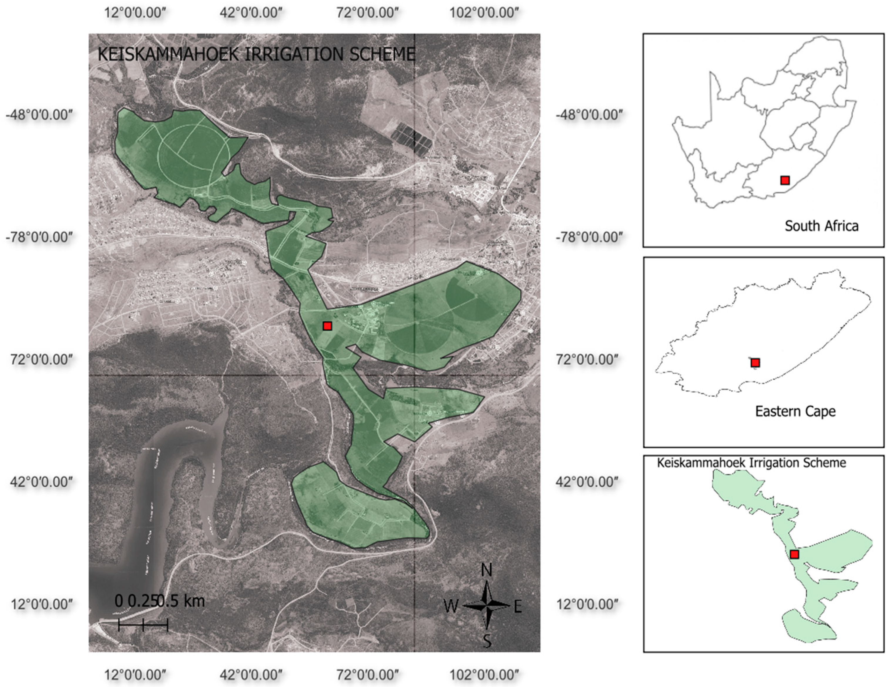
Figure 1. Keiskammahoek Irrigation Scheme map marked with gray colour.
Hydrology 11 00176 g001
Figure 2. Shows the BAST graphs for ET (a), NDWI (b), P (c), NDVI (d), MV (e), and SF (f).
Hydrology 11 00176 g002
Figure 3. ET (a) and P (b) normalised wavelet power spectra of yearly mean variability during 2001 to 2018 at KIS.
Hydrology 11 00176 g003
Figure 4. Wavelet coherence between ET and precipitation for period of 2001 to 2018 with phase relationship depicted by the arrows.
Hydrology 11 00176 g004
Figure 5. Pearson Correlation Coefficient for NDDI, ET, NDVI, NDWI, SF, and P.
Hydrology 11 00176 g005
Figure 6. Long-term trend of monthly SF (a), MV (b), ET (c), and P (d).
Hydrology 11 00176 g006
Figure 7. SQ-MK test for ET and P data for trend period in years 2001–2018. The sequent statistics values of progressive (Prog) u(t) (red solid line) and retrograde u’(t) (solid black line) attained by the Sequential Man-Kendal (SQ-) test for ET data (a) and Precipitation data (b) for 18 years period.
Hydrology 11 00176 g007
Figure 8. Autocorrelation Function (ACF) (a) and the histogram of residuals (b) for KIS for the 18 years (2001 to 2018) showing a Keiskammahoek Irrigation Scheme best fitted model for ET data series.
Hydrology 11 00176 g008
Figure 9. (a) ET dataset from 2001 to 2018 and 3-year forecast from 2015 to 2028, and (b) ARIMA scatter plot with correlation between forecasted ET and obtained ET.
Hydrology 11 00176 g009
Figure 10. (a) ET dataset from 2001 to 2015 and the remaining forecasted from 2015 to 2018, and (b) ANN scatter plot with correlation between forecasted ET and obtained ET.
Hydrology 11 00176 g010
Table 1. Long-term trend of monthly ET, precipitation, SF, MV, NDVI, NDWI, and NDDI.
VariablesZ-ScoreKendall’s TauSVar(S)p-Value
ET3.8981.782946 × 10−14.140000 × 1031.127460 × 1069.698 × 10−5
Precipitation−2.6134−1.195521 × 10⁻¹−2.7760001.127460 × 1060.008964
SF−1.7508−8.016553 × 10⁻²−1.860000 × 1031.127368 × 1060.07997
MV0.607472.785445 × 10−26.460000 × 1021.127391 × 1060.5435
NDVI8.32913.809626 × 10−18.845000 × 1031.127455 × 1062.2 × 10−16
NDWI10.0214.583118 × 10−11.061200 × 1041.127460 × 1062.2 × 10−16
NDDI−9.8859−4.521102 × 10⁻¹−1.049800 × 1041.127460 × 1062.2 × 10−16
Table 2. MLR model showing ET is the dependent variable and SF, P, NDVI, NDWI, and NDDI are independent variables.
ParametersEstimateStd. Errort ValuePr-ValueSig
ET3.40761970.200974016.956<2 × 10⁻¹⁶***
SF−0.01565140.0032221−4.8572.32 × 10−6***
Precipitation0.00454860.000431810.534<2 × 10⁻¹⁶***
NDVI2.75646010.40222616.8537.89 × 10−11***
NDWI−0.32027770.5270840−0.6080.5441
NDDI−0.29015420.1246038−2.3290.0208*
Table 3. Results of the four performance evaluators adopted in this study.
ModelsRMSEMAEMAPER
ARIMA37.5832.3717.260.94
ANN44.1835.8824.350.86
Disclaimer/Publisher’s Note: The statements, opinions and data contained in all publications are solely those of the individual author(s) and contributor(s) and not of MDPI and/or the editor(s). MDPI and/or the editor(s) disclaim responsibility for any injury to people or property resulting from any ideas, methods, instructions or products referred to in the content.