

Modeling Large River Basins and Flood Plains with Scarce Data: Development of the Large Basin Data Portal


Abstract
1. Introduction
2. Materials and Methods
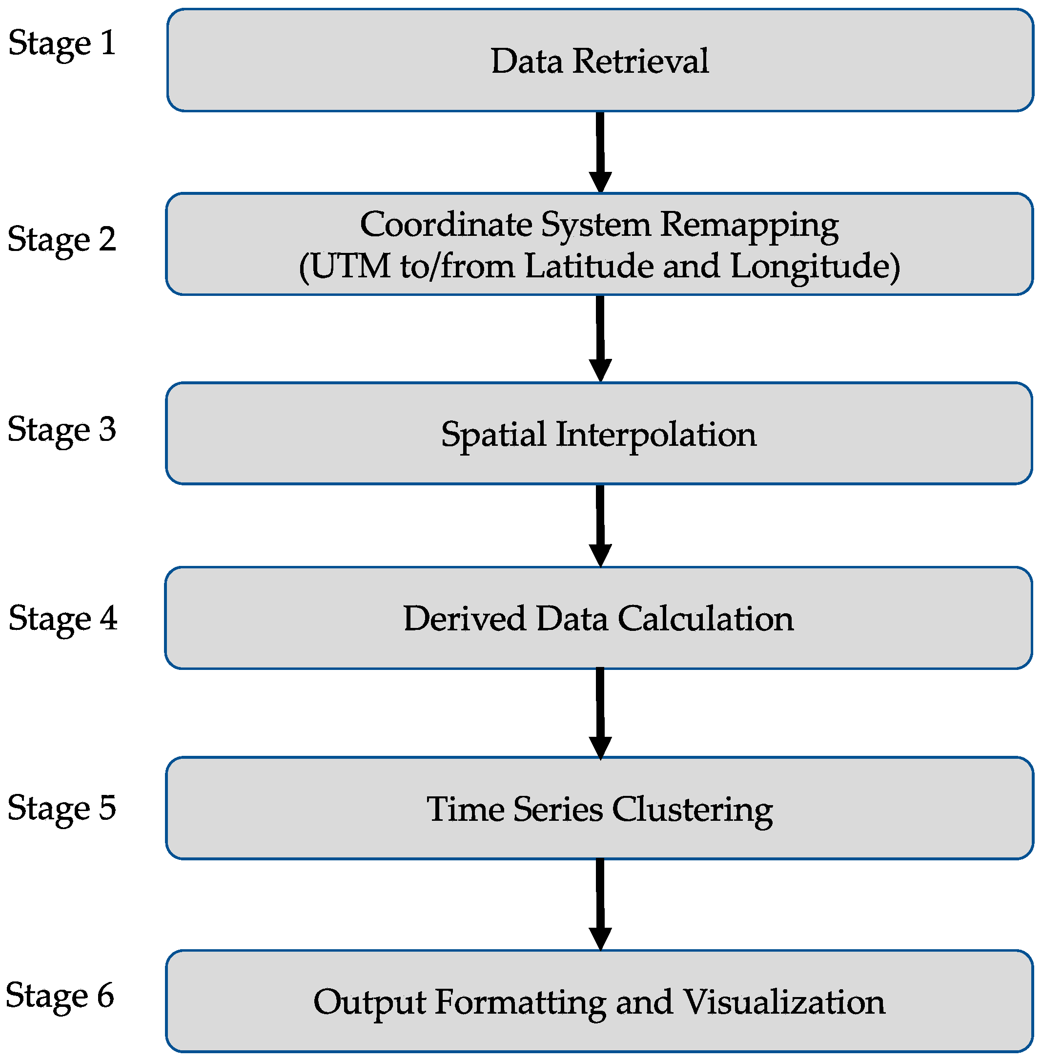
2.1. Data Processing Stages
2.1.1. Stage 1—Data Retrieval
2.1.2. Stage 2—Coordinate System Remapping
2.1.3. Stage 3—Linear Spatial Interpolation
2.1.4. Stage 4—Derived Data Calculation
2.1.5. Stage 5—Time Series Clustering
2.1.6. Stage 6—Output Data Formatting
2.2. Output Data Validation
2.3. Large Basin Data Portal—Data Extraction Tools
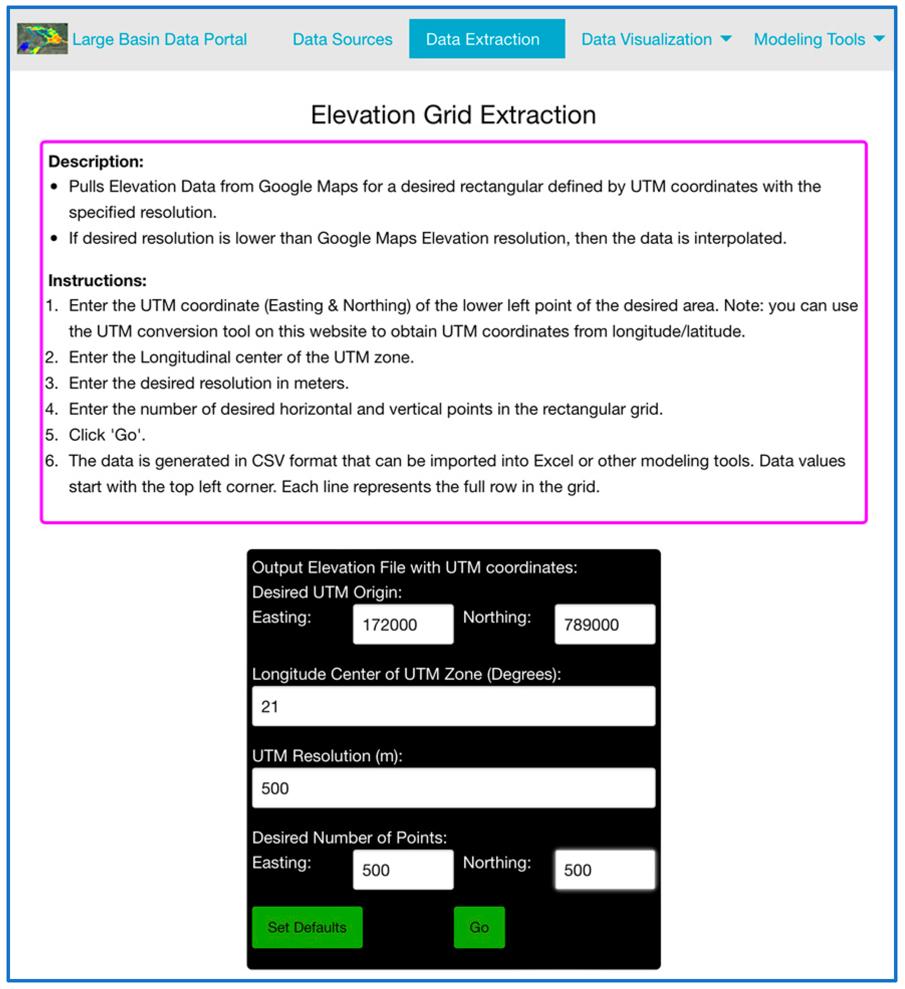
2.3.1. Elevation Grid Extraction
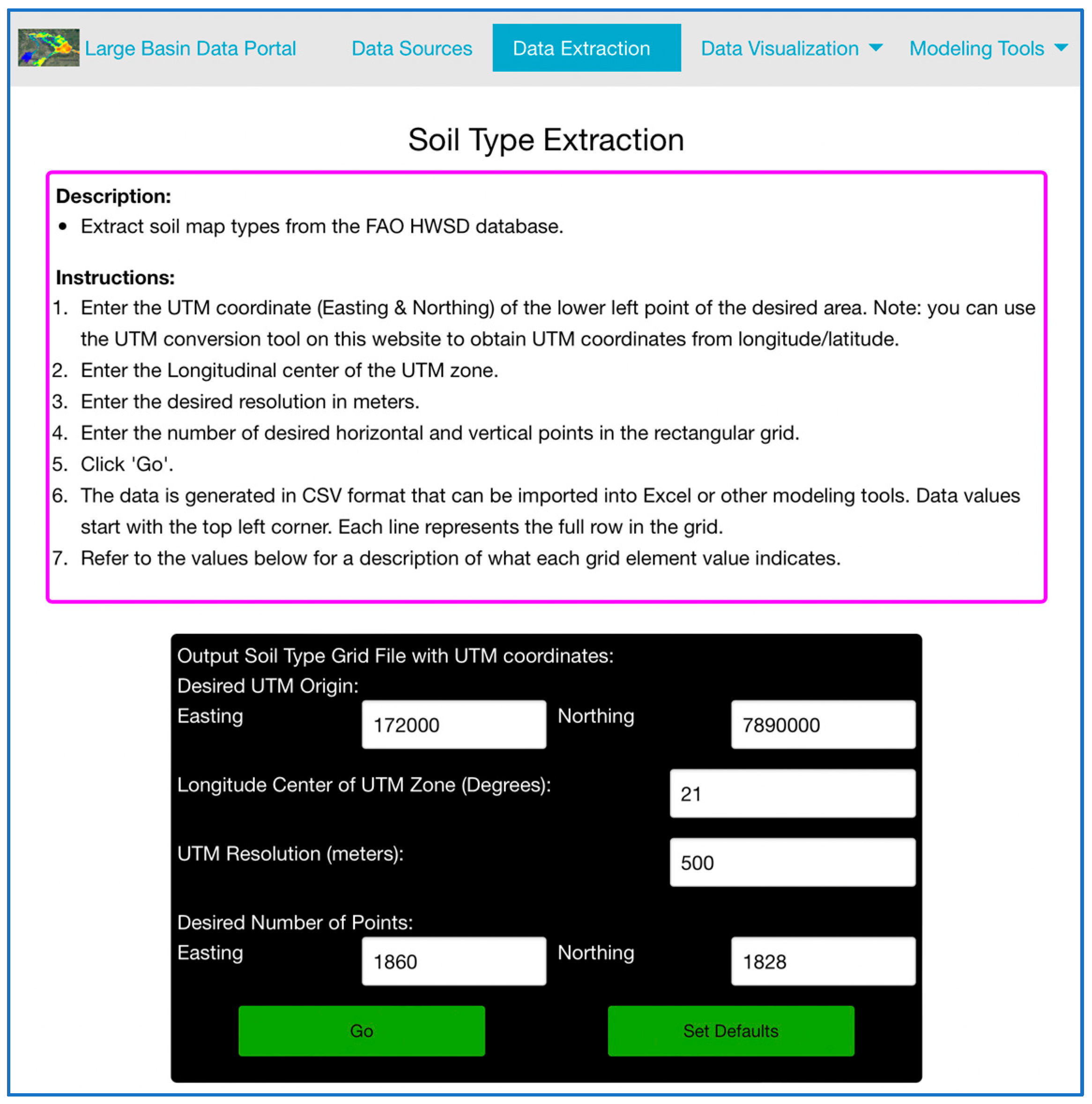
2.3.2. Soil Type Extraction
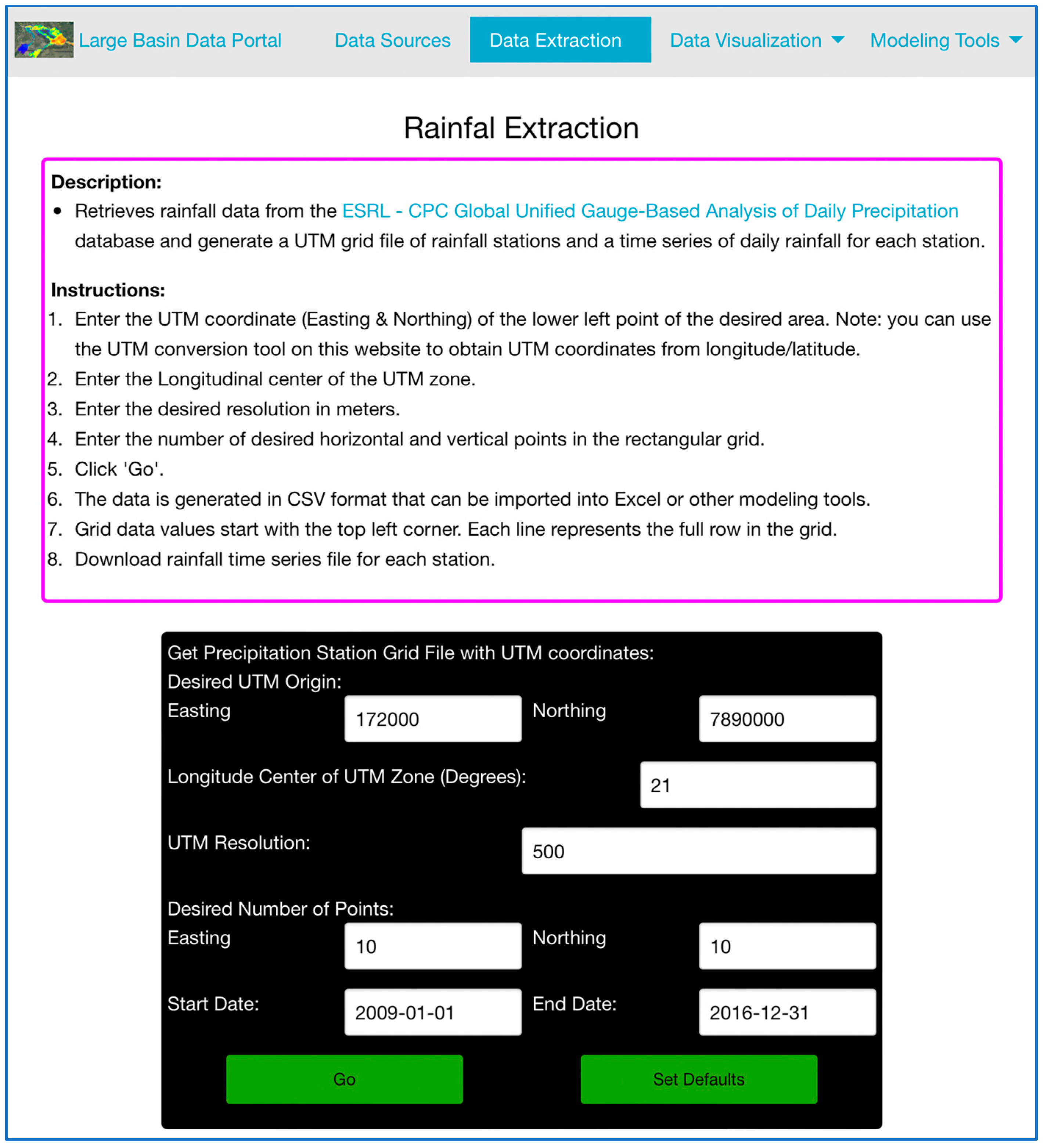
2.3.3. Rainfall Extraction
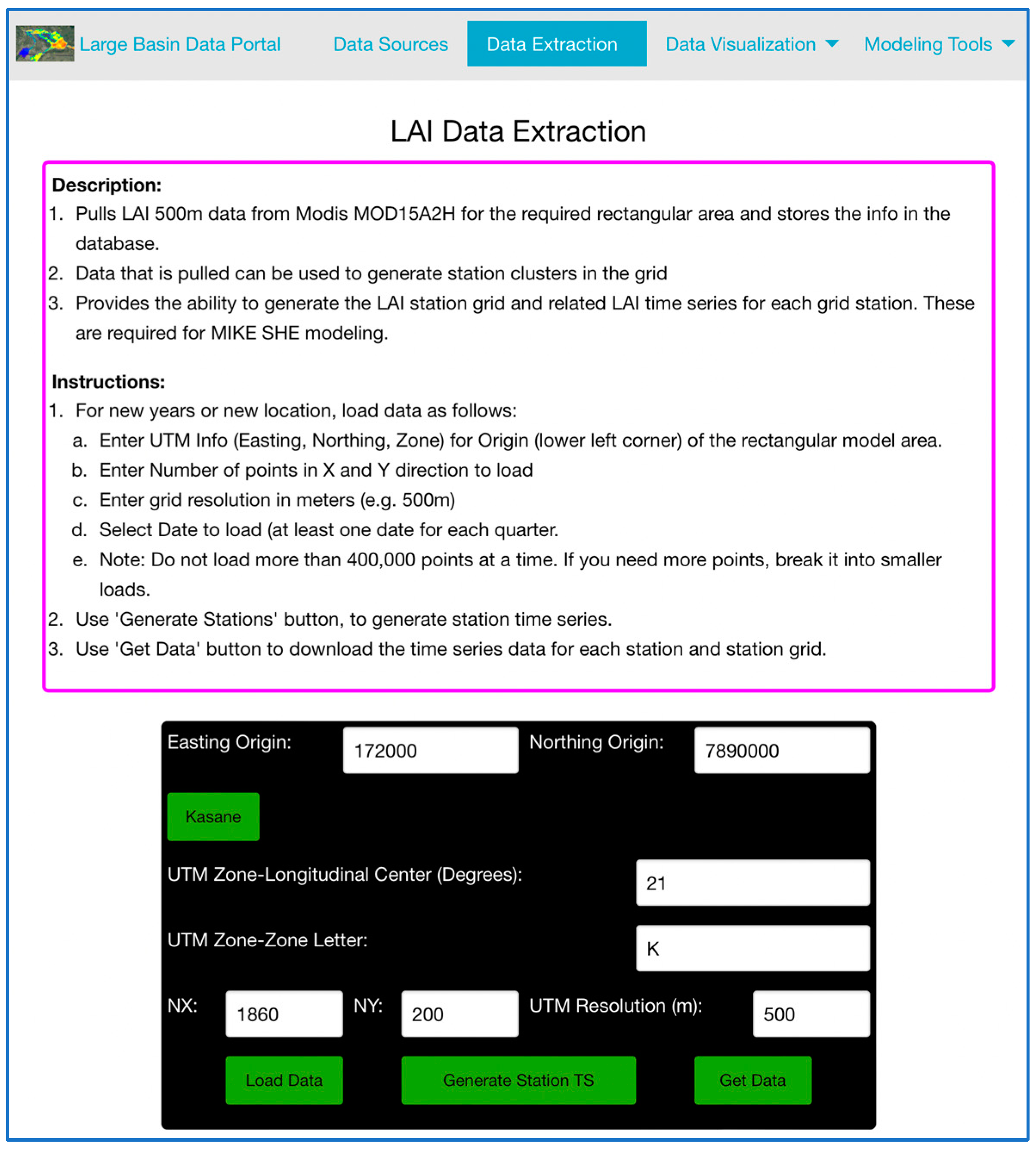
2.3.4. Leaf Area Index (LAI) Data Extraction
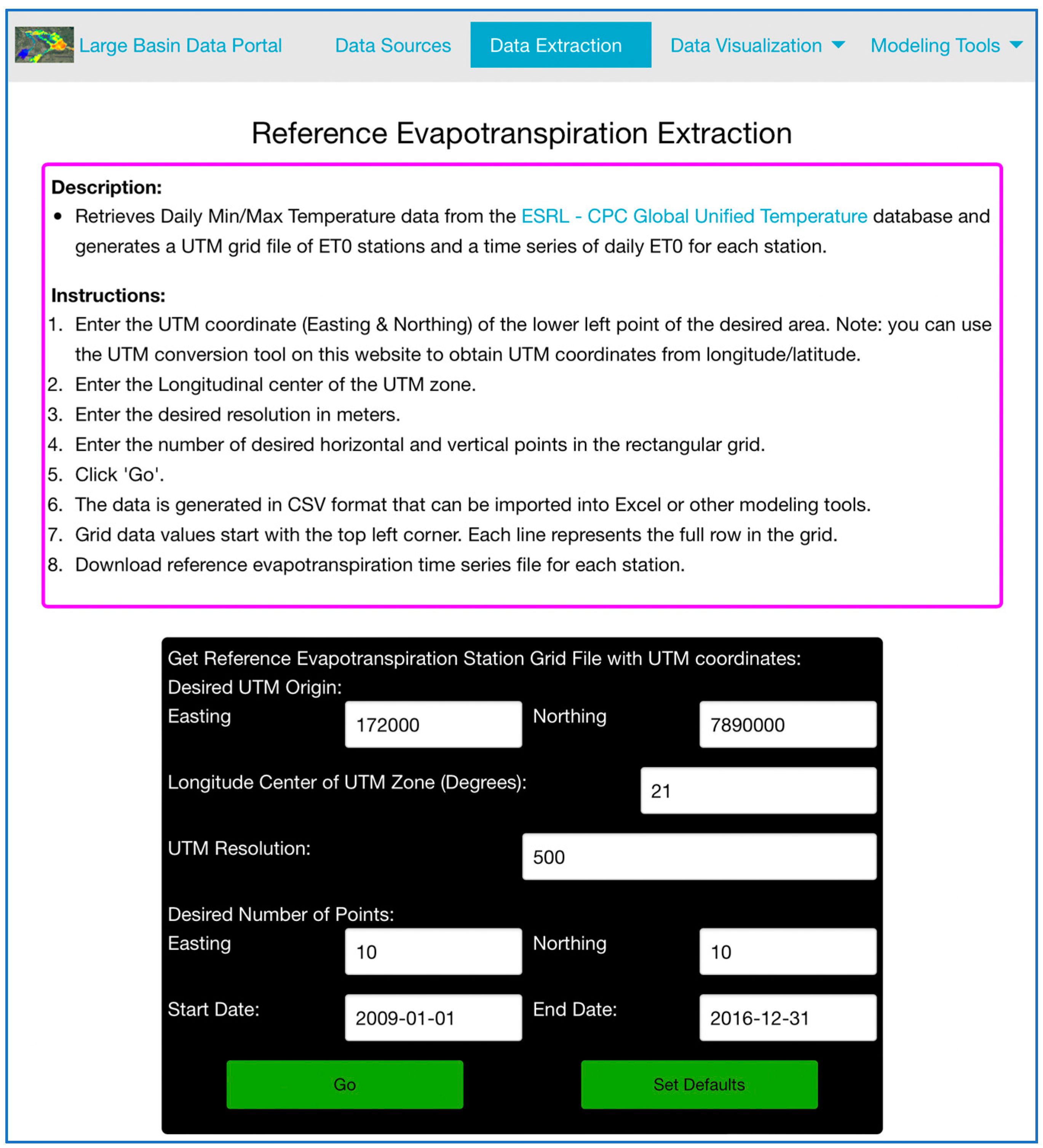
2.3.5. Reference Evapotranspiration Data Extraction
2.4. Large Basin Data Portal—Data Visualization Tools
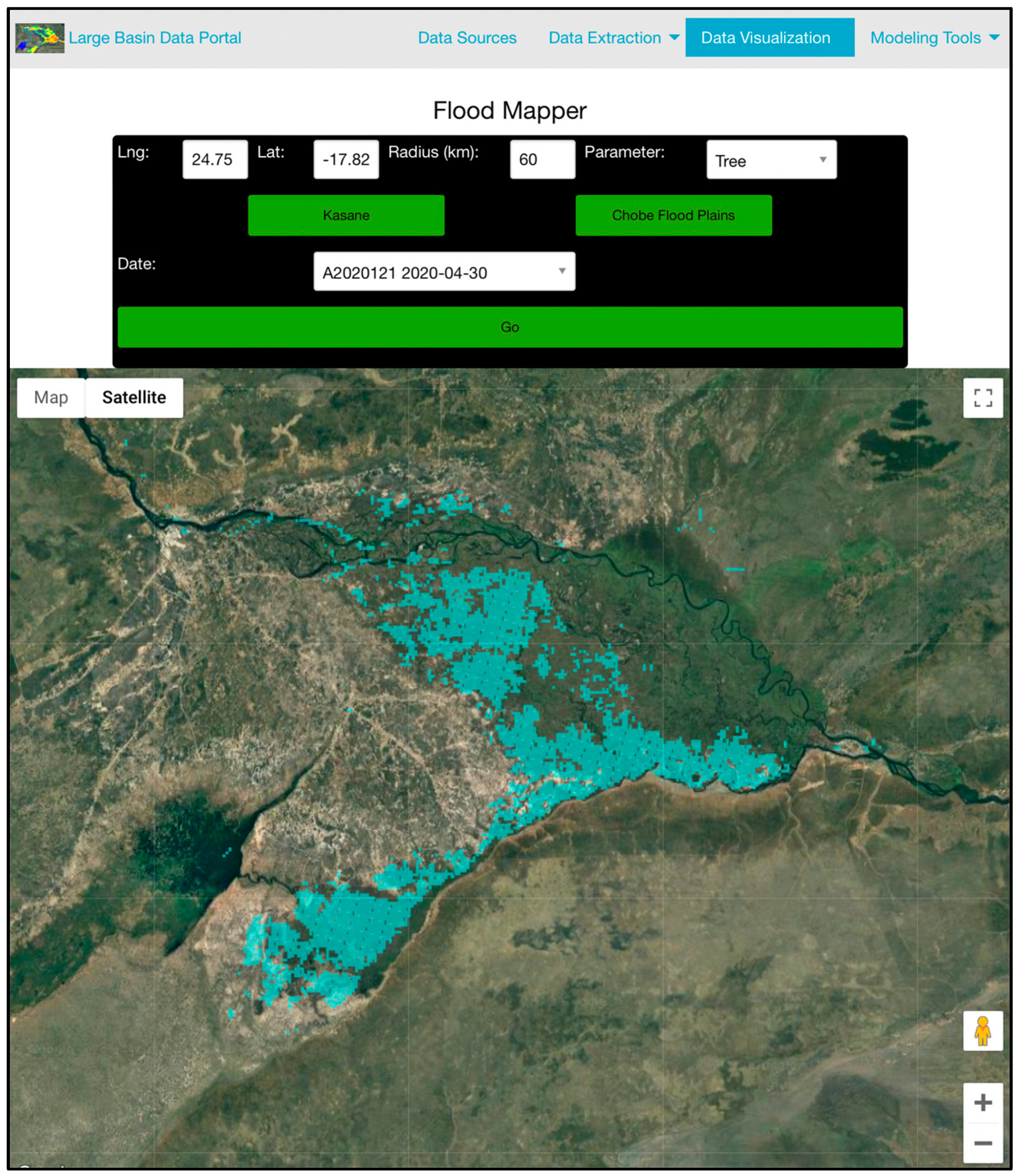
2.4.1. Flood Mapper
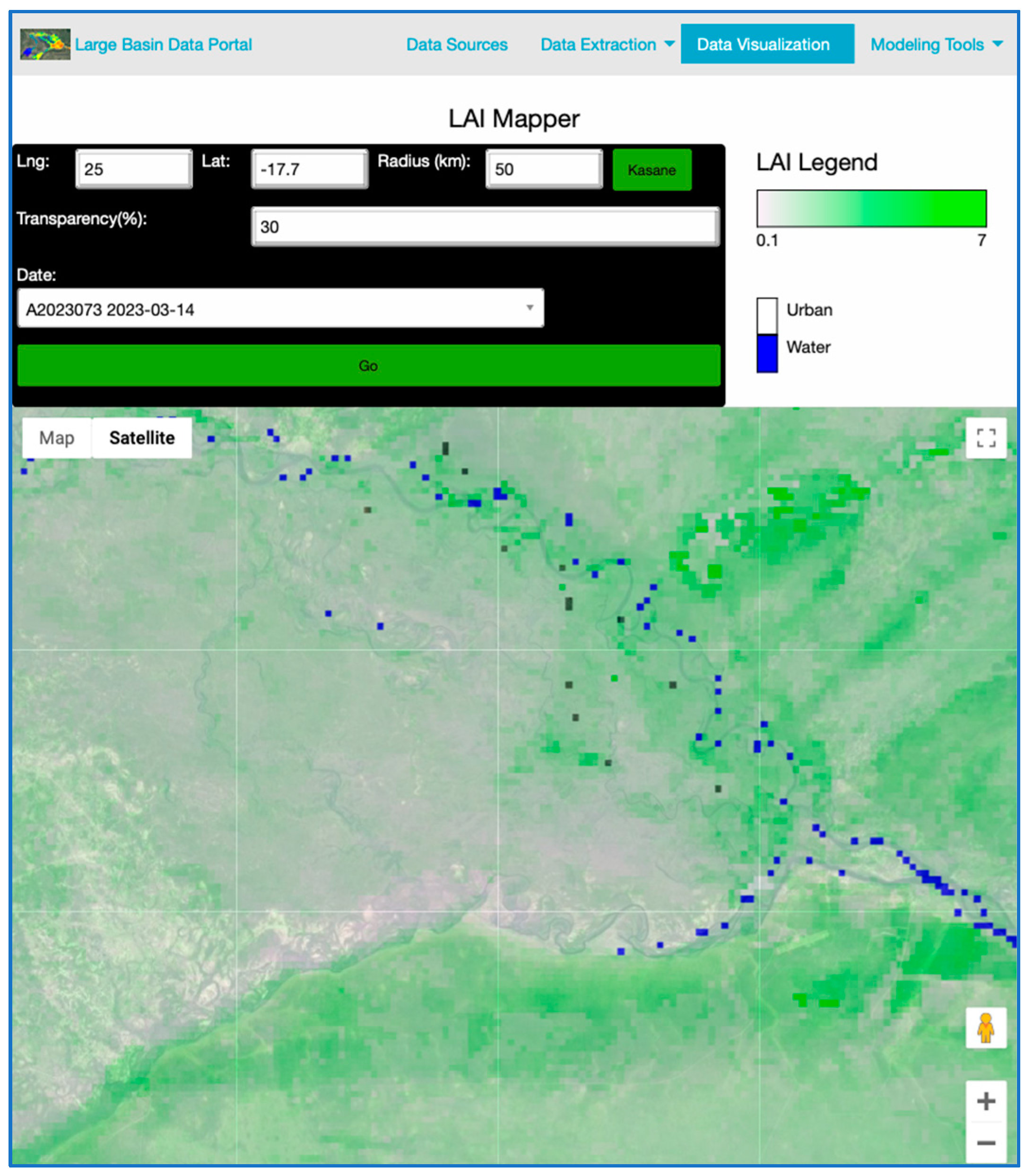
2.4.2. LAI Mapper
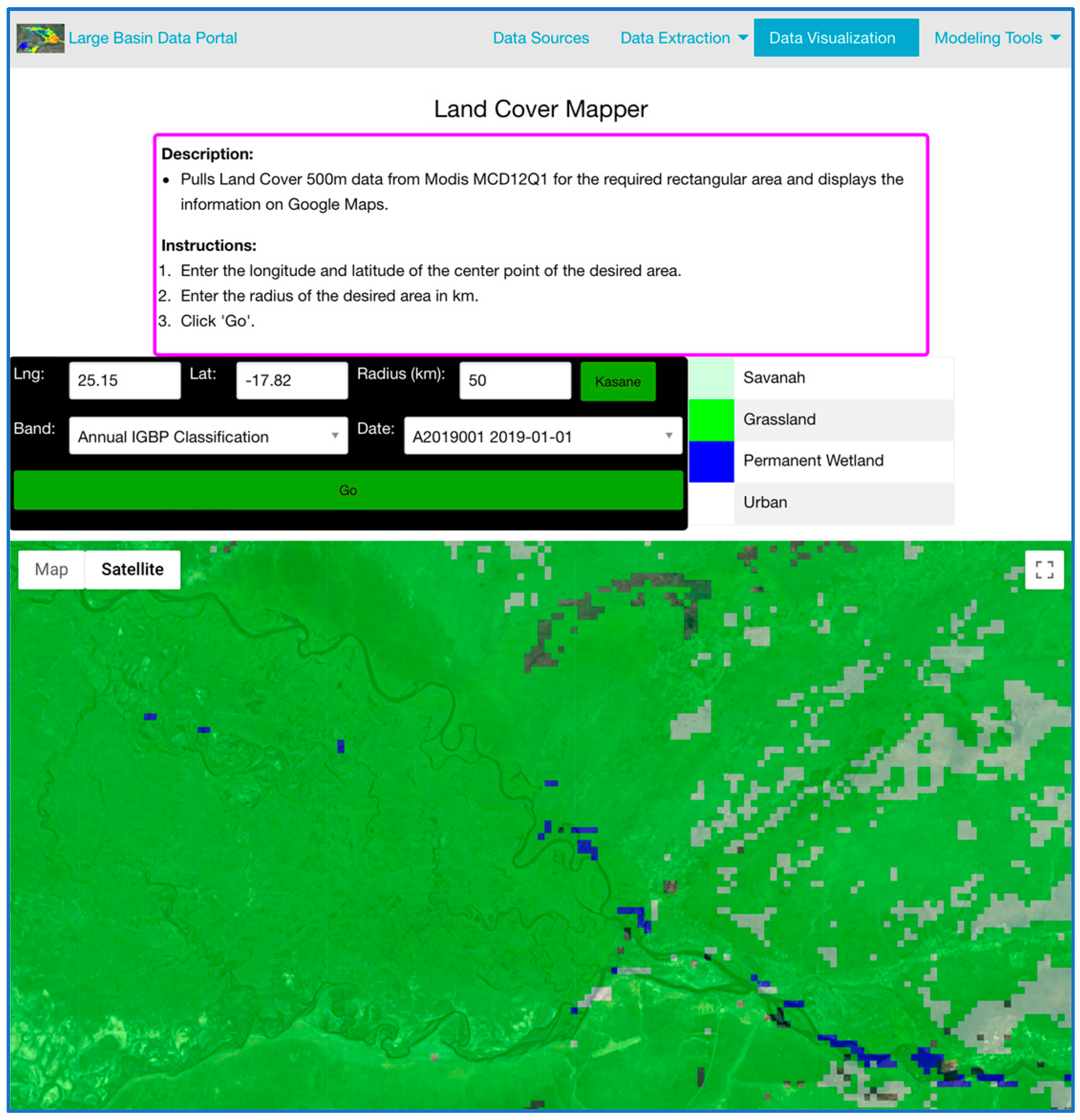
2.4.3. Land Cover Mapper
2.5. Large Basin Data Portal—Other Modeling Tools
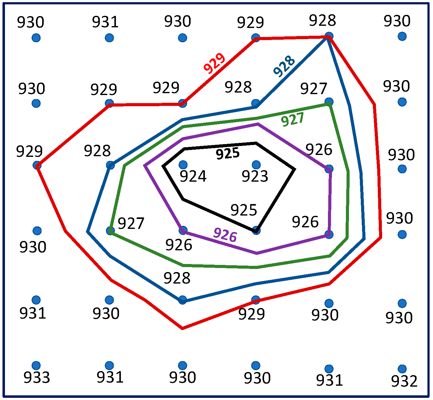
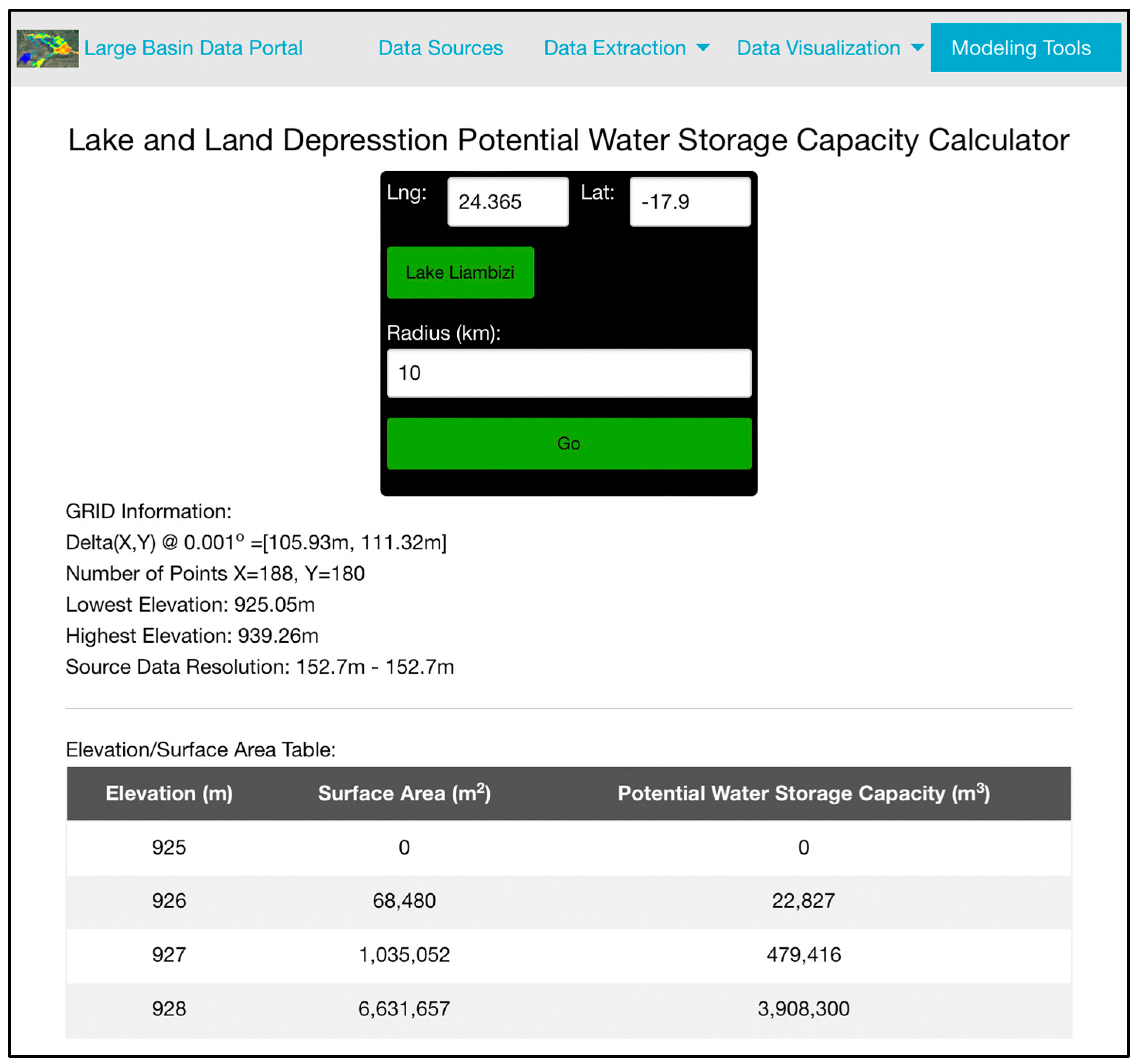
2.5.1. Lake and Land Depression Water Storage Capacity Calculator
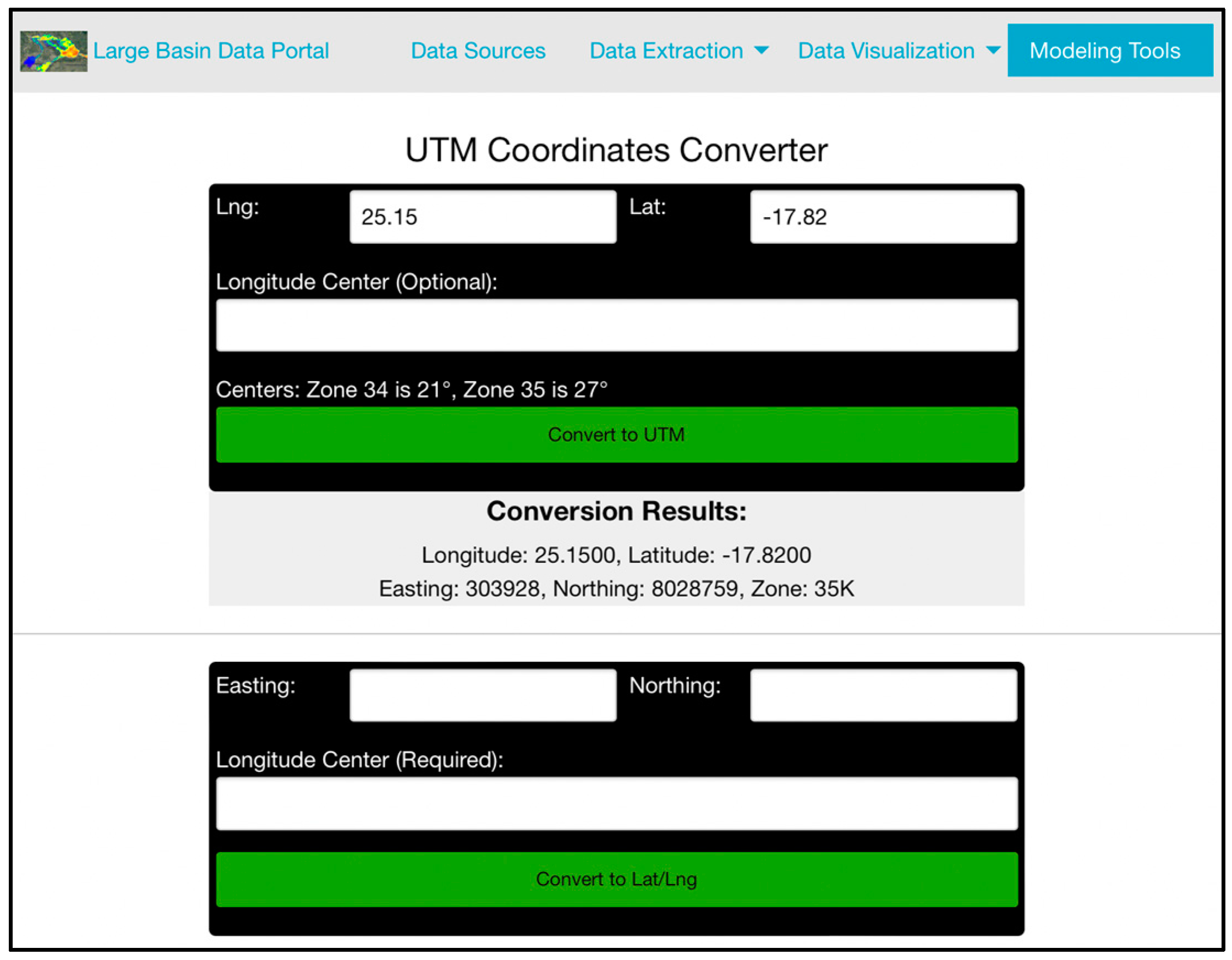
2.5.2. UTM Coordinates Convertor
2.6. Large Basin Data Portal—Database of Data Sources for Modeling
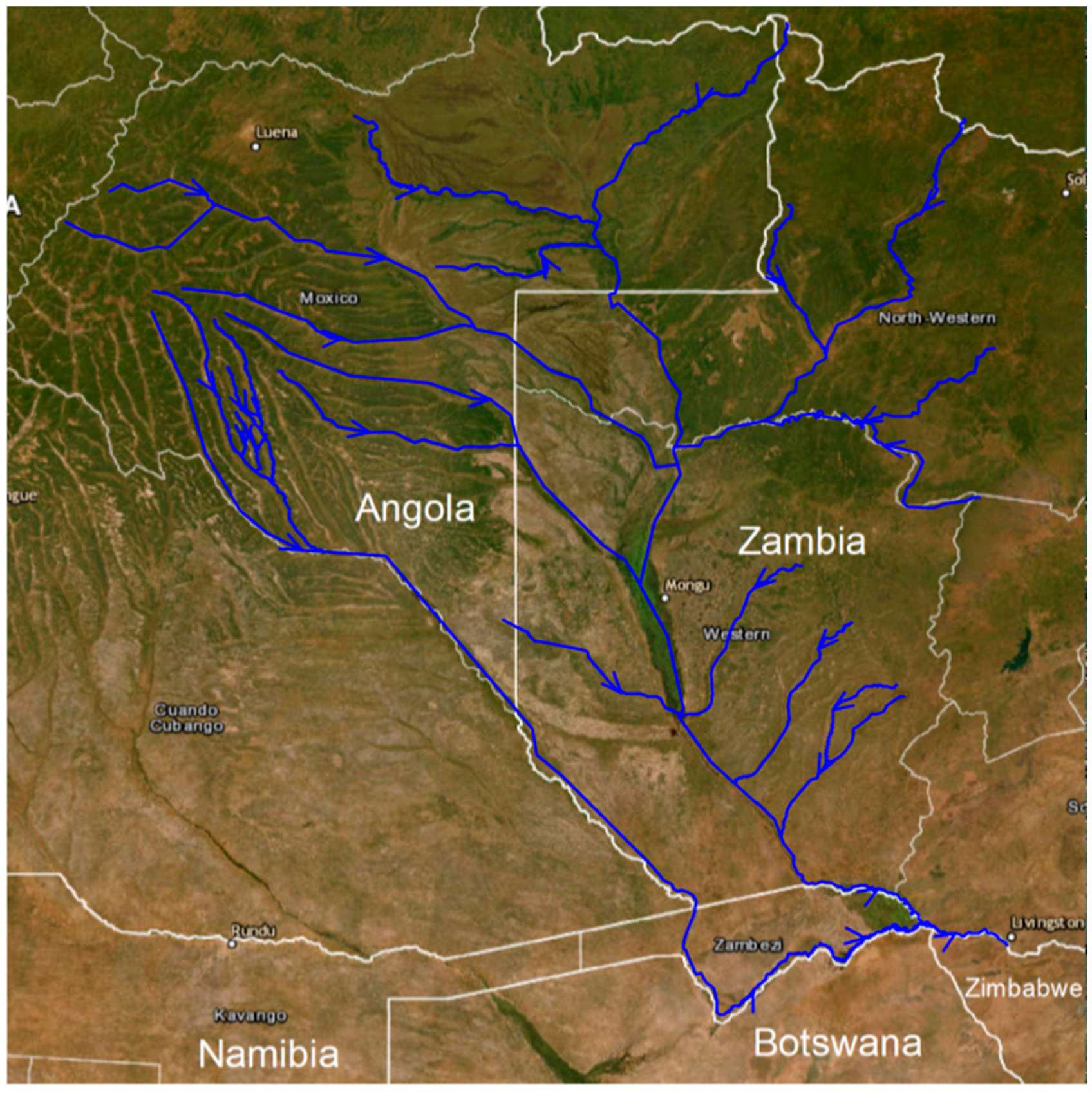
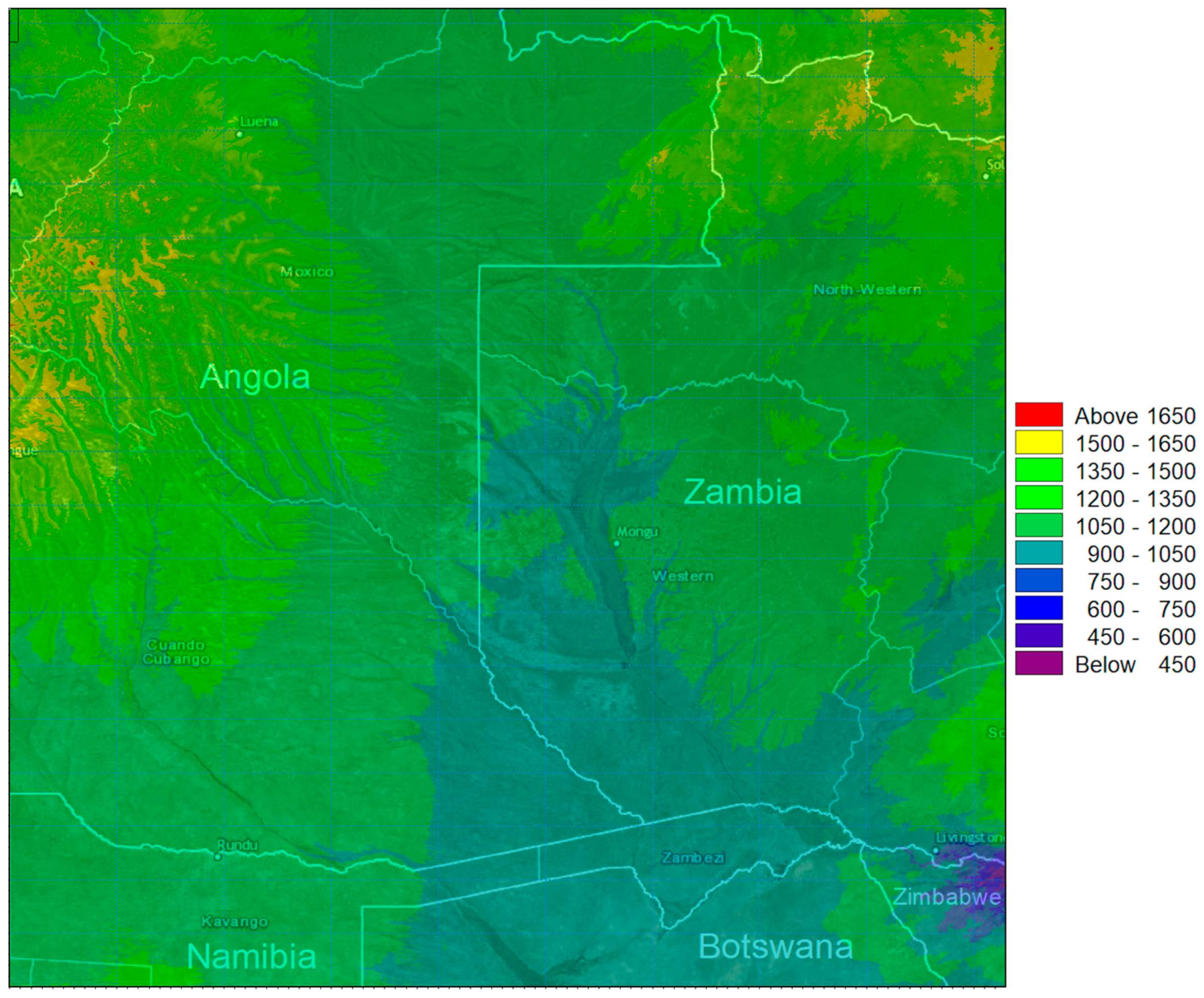
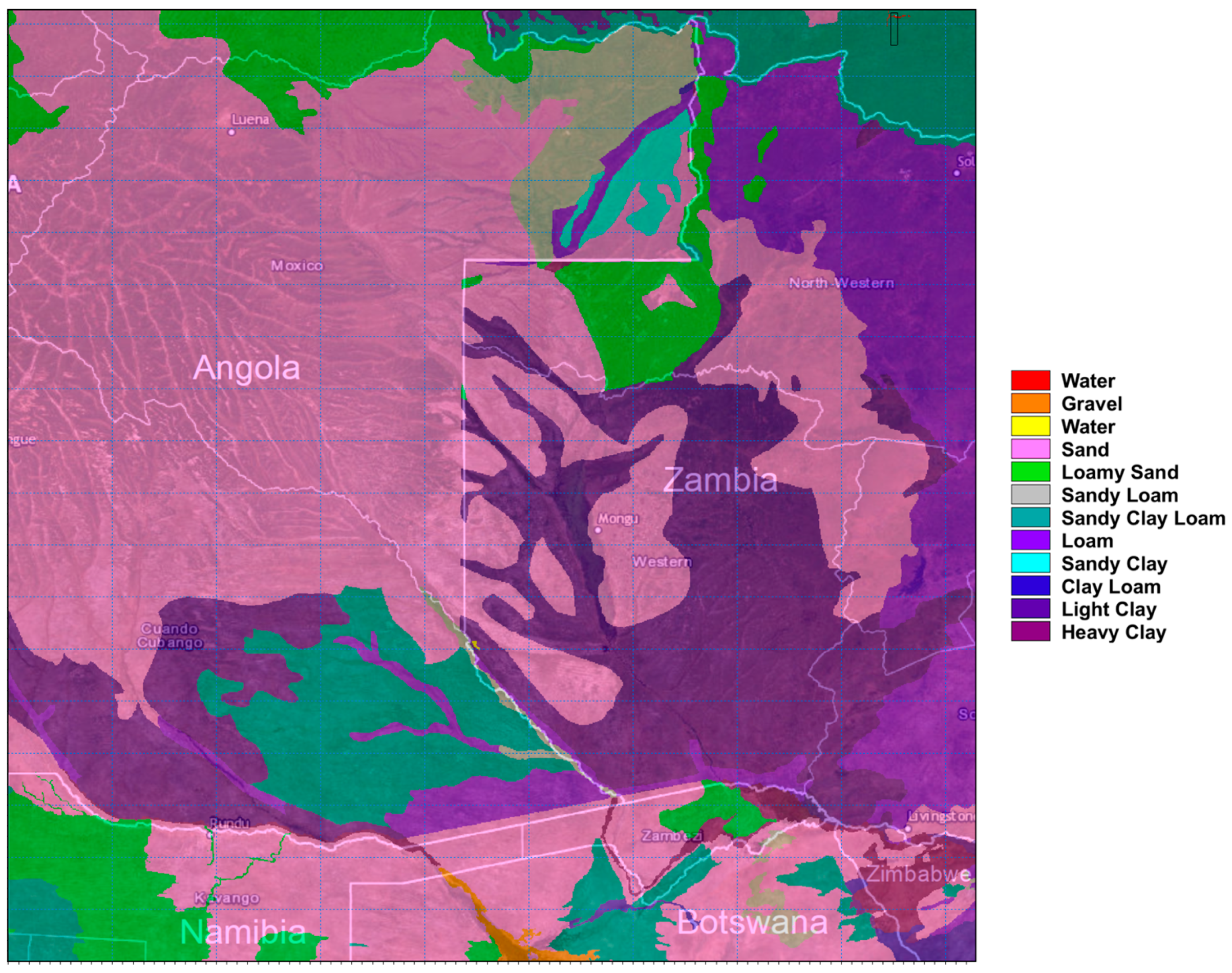
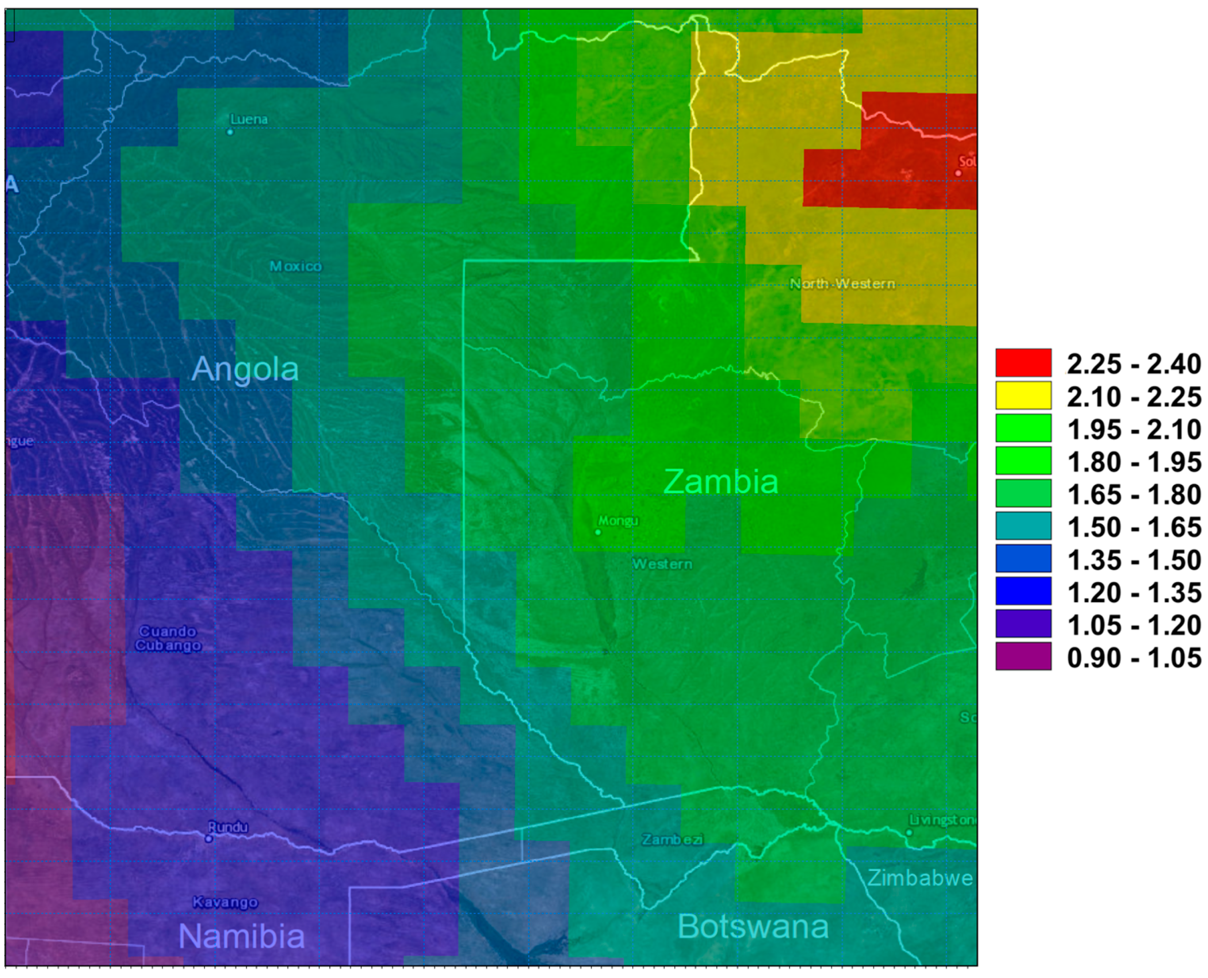
3. Results—Case Study: The Upper Zambezi River Basin Region
4. Discussion
5. Conclusions
Supplementary Materials
Author Contributions
Funding
Data Availability Statement
Conflicts of Interest
Appendix A

| Category | Data Type | Source and Dataset | Temporal Resolution | Time Period | Spatial Resolution | Spatial Coverage |
|---|---|---|---|---|---|---|
| Climate | Evaporation | European Centre for Medium-Range Weather Forecasts (ERA) | 6 h | 1979–Present | 80 km | Worldwide |
| Climate | Evaporation/Transpiration | Global Land Evaporation Amsterdam Model (GLEAM) | Daily | 1980–Present | 0.25° | Worldwide |
| Climate | Evapotranspiration | MODIS (MOD16A2) | 8-Day | 2001–Present | 500 m | Worldwide |
| Climate | Precipitation | Nicholson African Monthly Rainfall Database | Monthly | 1901–1984 | Scattered Weather Monitoring Stations | Africa |
| Climate | Precipitation | WorldClim | Monthly | 1970–2000 | 30 arc s | Worldwide |
| Climate | Precipitation | ESRL | Daily 1 | 1979–Present (1) | 0.5° 1 | Worldwide |
| Climate | Precipitation | National Centers for Environmental Information | Hourly/Daily | Varies by location | Scattered Weather Monitoring Stations | Worldwide |
| Climate | Precipitation | European Centre for Medium-Range Weather Forecasts (ERA) | 6 h | 1979–Present | 0.4° | Worldwide |
| Climate | Precipitation | NASA Global Precipitation Measurement | 30 min 1 | 2000–Present (1) | 0.1° 1 | Worldwide |
| Climate | Solar Radiation | WorldClim | Monthly | 1970–2000 | 30 arc s | Worldwide |
| Climate | Temperature | European Centre for Medium-Range Weather Forecasts ERA | 6 h | 1979–Present | 0.4° | Worldwide |
| Climate | Temperature | National Centers for Environmental Information | Hourly/Daily | Varies by location | Scattered Weather Monitoring Stations | Worldwide |
| Climate | Temperature (Land Surface) | MODIS (MOD11A2) | 8-Day | 2000–Present | 1 km | Worldwide |
| Climate | Temperature Min/Max | ESRL | Daily 1 | 1979–Present 1 | 0.5° 1 | Worldwide |
| Climate | Temperature Min/Max | WorldClim | Monthly | 1970–2000 | 30 arc s | Worldwide |
| Climate | Water Vapor Pressure | WorldClim | Monthly | 1970–2000 | 30 arc s | Worldwide |
| Climate | Wind Speed | European Centre for Medium-Range Weather Forecasts (ERA) | 6 h | 1979–Present | 0.4° | Worldwide |
| Climate | Wind Speed | WorldClim | Monthly | 1970–2000 | 30 arc s | Worldwide |
| Land Cover | LAI | MODIS (MOD15A2H) | 8-Day | 2002–Present | 500 m | Worldwide |
| Land Cover | Land Cover | FAO HWSD | N/A | N/A | 30 arc s | Worldwide |
| Land Cover | Land Cover Type | MODIS (MCD12Q1) | Yearly | 2001–Present | 500 m | Worldwide |
| Land Cover | Vegetation Indices | MODIS (MOD13Q1) | 16-Day | 2000–Present | 250 m | Worldwide |
| Soil | Soil Type | FAO HWSD | N/A | N/A | 30 arc s | Worldwide |
| Surface Reflectance | Surface Reflectance | MODIS (MOD09A1) | 8-Day | 2002–Present | 500 m | Worldwide |
| Topography | Elevation | Google Maps Elevation | N/A | N/A | 3 arc s | Worldwide |
| Topography | Elevation | NASA Shuttle Radar Topographic Mission | N/A | N/A | 3 arc s | Worldwide |
| Topography | Elevation | FAO HWSD | N/A | N/A | 30 arc s | Worldwide |
References
- Cook, S.E.; Fisher, M.J.; Andersson, M.S.; Rubiano, J.; Giordano, M. Water, food and livelihoods in river basins. Water Int. 2009, 34, 13–29. [Google Scholar] [CrossRef]
- Loomis, J.; Kent, P.; Strange, L.; Fausch, K.; Covich, A. Measuring the total economic value of restoring ecosystem services in an impaired river basin: Results from a contingent valuation survey. Ecol. Econ. 2000, 33, 103–117. [Google Scholar] [CrossRef]
- Yang, J.; Xie, B.; Zhang, D.; Tao, W. Climate and land use change impacts on water yield ecosystem service in the Yellow River Basin, China. Environ. Earth Sci. 2021, 80, 72. [Google Scholar] [CrossRef]
- Rimal, B.; Sharma, R.; Kunwar, R.; Keshtkar, H.; Stork, N.E.; Rijal, S.; Rahman, S.A.; Baral, H. Effects of land use and land cover change on ecosystem services in the Koshi River Basin, Eastern Nepal. Ecosyst. Serv. 2019, 38, 100963. [Google Scholar] [CrossRef]
- Jain, C.K.; Singh, S. Impact of climate change on the hydrological dynamics of River Ganga, India. J. Water Clim. Chang. 2018, 11, 274–290. [Google Scholar] [CrossRef]
- Rocco, M.; Byron, O. Chapter Four—Hydrodynamic Modeling and Its Application in AUC. In Methods in Enzymology; Cole, J.L., Ed.; Academic Press: Cambridge, MA, USA, 2015; Volume 562, pp. 81–108. [Google Scholar]
- Yamamoto, K.; Sayama, T.; Apip. Impact of climate change on flood inundation in a tropical river basin in Indonesia. Prog. Earth Planet. Sci. 2021, 8, 5. [Google Scholar] [CrossRef]
- Lim, T.; Spokas, K.; Feyereisen, G.; Novak, J. Predicting the impact of biochar additions on soil hydraulic properties. Chemosphere 2016, 142, 136–144. [Google Scholar] [CrossRef]
- Garg, K.K.; Karlberg, L.; Barron, J.; Wani, S.P.; Rockstrom, J. Assessing impacts of agricultural water interventions in the Kothapally watershed, Southern India. Hydrol. Process. 2012, 26, 387–404. [Google Scholar] [CrossRef]
- Taylor, J.; Lai, K.M.; Davies, M.; Clifton, D.; Ridley, I.; Biddulph, P. Flood management: Prediction of microbial contamination in large-scale floods in urban environments. Environ. Int. 2011, 37, 1019–1029. [Google Scholar] [CrossRef]
- Alexander, K.A.; Heaney, A.K.; Shaman, J. Hydrometeorology and flood pulse dynamics drive diarrheal disease outbreaks and increase vulnerability to climate change in surface-water-dependent populations: A retrospective analysis. PLoS Med. 2018, 15, e1002688. [Google Scholar] [CrossRef]
- Hussainzada, W.; Lee, H.S. Hydrological Modelling for Water Resource Management in a Semi-Arid Mountainous Region Using the Soil and Water Assessment Tool: A Case Study in Northern Afghanistan. Hydrology 2021, 8, 16. [Google Scholar] [CrossRef]
- Bharati, L.; Rodgers, C.; Erdenberger, T.; Plotnikova, M.; Shumilov, S.; Vlek, P.; Martin, N. Integration of economic and hydrologic models: Exploring conjunctive irrigation water use strategies in the Volta Basin. Agric. Water Manag. 2008, 95, 925–936. [Google Scholar] [CrossRef]
- Lund, J.R.; Palmer, R.N. Water Resource System M odeling for Conflict Resolution. Water Resour. Update 1997, 3, 70–82. [Google Scholar]
- Nishat, B.; Rahman, S.M.M. Water Resources Modeling of the Ganges-Brahmaputra-Meghna River Basins Using Satellite Remote Sensing Data1. JAWRA J. Am. Water Resour. Assoc. 2009, 45, 1313–1327. [Google Scholar] [CrossRef]
- Dile, Y.T.; Srinivasan, R. Evaluation of CFSR climate data for hydrologic prediction in data-scarce watersheds: An application in the Blue Nile River Basin. JAWRA J. Am. Water Resour. Assoc. 2014, 50, 1226–1241. [Google Scholar] [CrossRef]
- de Paiva, R.C.D.; Buarque, D.C.; Collischonn, W.; Bonnet, M.-P.; Frappart, F.; Calmant, S.; Bulhões Mendes, C.A. Large-scale hydrologic and hydrodynamic modeling of the Amazon River basin. Water Resour. Res. 2013, 49, 1226–1243. [Google Scholar] [CrossRef]
- Pricope, N.G. Variable-source flood pulsing in a semi-arid transboundary watershed: The Chobe River, Botswana and Namibia. Environ. Monit Assess 2013, 185, 1883–1906. [Google Scholar] [CrossRef]
- Burke, J.J. Modeling Surface Inundation and Flood Risk in a Flood-Pulsed Savannah: Chobe River, Botswana and Namibia; University of North Carolina Wilmington: Wilmington, NC, USA, 2015. [Google Scholar]
- Burke, J.J.; Pricope, N.G.; Blum, J. Thermal Imagery-Derived Surface Inundation Modeling to Assess Flood Risk in a Flood-Pulsed Savannah Watershed in Botswana and Namibia. Remote Sens. 2016, 8, 676. [Google Scholar] [CrossRef]
- Long, S.; Fatoyinbo, T.E.; Policelli, F. Flood extent mapping for Namibia using change detection and thresholding with SAR. Environ. Res. Lett. 2014, 9, 035002. [Google Scholar] [CrossRef]
- McCarthy, J.M.; Gumbricht, T.; McCarthy, T.; Frost, P.; Wessels, K.; Seidel, F. Flooding Patterns of the Okavango Wetland in Botswana between 1972 and 2000. AMBIO J. Hum. Environ. 2003, 32, 453–457. [Google Scholar] [CrossRef]
- Braget, M.P.; Goodin, D.G.; Wang, J.; Hutchinson, J.M.S.; Alexander, K. Flooded area classification using pooled training samples: An example from the Chobe River Basin, Botswana. J. Appl. Remote Sens. 2018, 12, 026033. [Google Scholar] [CrossRef]
- Geleta, H.I. Watershed Sediment Yield Modeling for Data Scarce Areas; Universitat Stuttgart: Stuttgart, Germany, 2011. [Google Scholar]
- Tegegne, G.; Park, D.K.; Kim, Y.-O. Comparison of hydrological models for the assessment of water resources in a data-scarce region, the Upper Blue Nile River Basin. J. Hydrol. Reg. Stud. 2017, 14, 49–66. [Google Scholar] [CrossRef]
- Chen, L.; Sun, C.; Wang, G.; Xie, H.; Shen, Z. Event-based nonpoint source pollution prediction in a scarce data catchment. J. Hydrol. 2017, 552, 13–27. [Google Scholar] [CrossRef]
- Johnston, R.; Smakhtin, V. Hydrological Modeling of Large river Basins: How Much is Enough? Water Resour. Manag. 2014, 28, 2695–2730. [Google Scholar] [CrossRef]
- Ireson, A.; Makropoulos, C.; Maksimovic, C. Water resources modelling under data scarcity: Coupling MIKE BASIN and ASM groundwater model. Water Resour. Manag. 2006, 20, 567–590. [Google Scholar] [CrossRef]
- Swain, S.S.; Mishra, A.; Sahoo, B.; Chatterjee, C. Water scarcity-risk assessment in data-scarce river basins under decadal climate change using a hydrological modelling approach. J. Hydrol. 2020, 590, 125260. [Google Scholar] [CrossRef]
- Zambezi River Authority: Geography of the Zambezi River. Available online: http://www.zambezira.org/hydrology/geography (accessed on 15 February 2023).
- Schultz, G.A. Hydrological modeling based on remote sensing information. Adv. Space Res. 1993, 13, 149–166. [Google Scholar] [CrossRef]
- Alexander, K.A.; Blackburn, J.K. Overcoming barriers in evaluating outbreaks of diarrheal disease in resource poor settings: Assessment of recurrent outbreaks in Chobe District, Botswana. BMC Public Health 2013, 13, 775. [Google Scholar] [CrossRef]
- Moore, A.E.; Cotterill, F.P.; Main, M.P.; Williams, H.B. The zambezi river. In Large Rivers: Geomorphology and Management; John Wiley & Sons: Hoboken, NJ, USA, 2007; pp. 311–332. [Google Scholar]
- Beyer, M.; Wallner, M.; Bahlmann, L.; Thiemig, V.; Dietrich, J.; Billib, M. Rainfall characteristics and their implications for rain-fed agriculture: A case study in the Upper Zambezi River Basin. Hydrol. Sci. J. 2016, 61, 321–343. [Google Scholar] [CrossRef]
- PHP: PHP Hypertext Processor. Available online: https://www.php.net/docs.php (accessed on 15 February 2023).
- The GNU C Reference Manual. Available online: https://www.gnu.org/software/gnu-c-manual/gnu-c-manual.html (accessed on 29 March 2023).
- Slater, J.A.; Malys, S. WGS 84—Past, Present and Future; SpringerLink: Berlin, Germany, 1998; pp. 1–7. [Google Scholar]
- Lu, G.Y.; Wong, D.W. An adaptive inverse-distance weighting spatial interpolation technique. Comput. Geosci. 2008, 34, 1044–1055. [Google Scholar] [CrossRef]
- DHI. MIKE-SHE (Version 2022). Windows. DHI. 2022. Available online: https://www.mikepoweredbydhi.com/download/mike-2022 (accessed on 8 March 2023).
- Lloyd, S. Least squares quantization in PCM. IEEE Trans. Inf. Theory 1982, 28, 129–137. [Google Scholar] [CrossRef]
- NASA: Flooding on the Zambezi River. Available online: https://earthobservatory.nasa.gov/images/83667/flooding-on-the-zambezi-river (accessed on 15 February 2023).
- Google. Google Maps Platforms. Available online: http://mapsplatform.google.com (accessed on 20 February 2023).
- FAO; IIASA; ISRIC; ISSCAS; JRC. Harmonized World Soil Database (Version 1.2). 2012. Available online: https://www.fao.org/soils-portal/data-hub/soil-maps-and-databases/harmonized-world-soil-database-v12/en/ (accessed on 20 February 2023).
- PSL, N.O.E. CPC US Unified Precipitation da. 2022. Available online: https://psl.noaa.gov/data/gridded/data.cpc.globalprecip.html (accessed on 20 February 2023).
- Myneni, R.; Knyazikhin, Y.; Park, T. MYD15A2H MODIS/Aqua Leaf Area Index/FPAR 8-Day L4 Global 500m SIN Grid. 2015. Available online: https://lpdaac.usgs.gov/products/myd15a2hv006/ (accessed on 20 February 2023). [CrossRef]
- Allan, R.; Pereira, L.; Smith, M. Crop Evapotranspiration-Guidelines for Computing Crop Water Requirements-FAO Irrigation and Drainage Paper 56; FAO: Rome, Italy, 1998; Volume 56. [Google Scholar]
- Hargreaves, G.; Samani, Z. Reference Crop Evapotranspiration From Temperature. Appl. Eng. Agric. 1985, 1, 96–99. [Google Scholar] [CrossRef]
- Vermote, E. MOD09A1 MODIS Surface Reflectance 8-Day L3 Global 500m SIN Grid V006. 2015. Available online: https://lpdaac.usgs.gov/products/mod09a1v006/ (accessed on 20 February 2023).
- Sun, D.; Yu, Y.; Goldberg, M.D. Deriving Water Fraction and Flood Maps From MODIS Images Using a Decision Tree Approach. IEEE J. Sel. Top. Appl. Earth Obs. Remote Sens. 2011, 4, 814–825. [Google Scholar] [CrossRef]
- Friedl, M.S.-M.D. MCD12Q1 MODIS/Terra+Aqua Land Cover Type Yearly L3 Global 500m SIN Grid V006. 2019. Available online: https://lpdaac.usgs.gov/products/mcd12q1v006/ (accessed on 20 February 2023).
- Taube, C.M. Instructions for winter lake mapping. In Manual of Fisheries Survey Methods II: With Periodic Updates; Schneider, J.C., Ed.; Fisheries Special Report 25; Michigan Department of Natural Resources: Ann Arbor, MI, USA, 2000; Chapter 12. [Google Scholar]
- Kelly, K.M. Universal Transverse Mercator/Geographic Coordinate Transformations; Ontario Ministry of Natural Resources: Vancouver, BC, Canada, 1986. [Google Scholar]
- Beilfuss, R. A Risky Climate for Southern African Hydro: Assessing hydrological risks and consequences for Zambezi River Basin Dams; International Rivers: Berkeley, CA, USA, 2012. [Google Scholar]
- Seipel, S.; Lim, N.J. Color map design for visualization in flood risk assessment. Int. J. Geogr. Inf. Sci. 2017, 31, 2286–2309. [Google Scholar] [CrossRef]
- Auliagisni, W.; Wilkinson, S.; Elkharboutly, M. Using community-based flood maps to explain flood hazards in Northland, New Zealand. Prog. Disaster Sci. 2022, 14, 100229. [Google Scholar] [CrossRef]
- Moughtin, C.; Oc, T.; Tiesdell, S. Urban Design: Ornament and Decoration; Routledge: Abingdon, UK, 1999. [Google Scholar]
- Khattab, M.F.; Abo, R.K.; Al-Muqdadi, S.W.; Merkel, B.J. Generate reservoir depths mapping by using digital elevation model: A case study of Mosul dam lake, Northern Iraq. Adv. Remote Sens. 2017, 6, 161–174. [Google Scholar] [CrossRef]
- Holst, K.A.; Madsen, H.B. The elaboration of drainage class maps for agricultural planning in Denmark. Landsc. Urban Plan. 1986, 13, 199–218. [Google Scholar] [CrossRef]
- Vella, S. Soil survey and soil mapping in the Maltese Islands: The 2003 position. Eur. Soil Bur. Res. Rep. 2003, 9, 235–244. [Google Scholar]
- Gosling, S.N.; Arnell, N.W. Simulating current global river runoff with a global hydrological model: Model revisions, validation, and sensitivity analysis. Hydrol. Process. 2011, 25, 1129–1145. [Google Scholar] [CrossRef]
- Nijssen, B.; O’Donnell, G.M.; Lettenmaier, D.P.; Lohmann, D.; Wood, E.F. Predicting the discharge of global rivers. J. Clim. 2001, 14, 3307–3323. [Google Scholar] [CrossRef]


| Data Source | Data Sets | Spatial and Temporal Resolution and Coverage | Data Retrieval Method |
|---|---|---|---|
| Moderate Resolution Imaging Spectroradiometer (MODIS) | MOD09A1 (Terra Surface Reflectance) | 500 m (Worldwide) 8-Day (2002–Present) | Location and time specific data retrieved automatically through the MODIS API when needed. |
| MCD12Q1 (Land Cover Type) | 500 m (Worldwide) Annual (2001–Present) | ||
| MOD15A2H (Terra Leaf Area Index) | 500 m (Worldwide) 8-Day (2002–Present) | ||
| Elevations | 3 arc s (Worldwide) | Location specific data retrieved through online API as needed. | |
| Earth System Research Laboratory (ESRL)—Climate Prediction Center (CPC) | CPC Global Precipitation | 0.5° (Worldwide) Daily (1979–Present) | Yearly global online dataset files are downloaded automatically when needed. |
| CPC Global Temperatures | 0.5° (Worldwide) Daily (1979–Present) | ||
| UN Food and Agriculture Organization (FAO) | Harmonized World Soil Database (HWSD) | 30 arc s (Worldwide) | Static dataset files have been pre-downloaded into the data portal. |
| R1 | R2 | R2–R1 | NDVI | NDWI | Classification |
|---|---|---|---|---|---|
| >9.17 | No Surface Water | ||||
| >6.45 | >0.5335 | No Surface Water | |||
| >2.91 | >0.228 | ≤0.2872 | No Surface Water | ||
| ≤1.02 | ≤2.91 | Water | |||
| ≤2.91 | <0.1509 | Water | |||
| ≤2.91 | >−0.2931 | Water |
Disclaimer/Publisher’s Note: The statements, opinions and data contained in all publications are solely those of the individual author(s) and contributor(s) and not of MDPI and/or the editor(s). MDPI and/or the editor(s) disclaim responsibility for any injury to people or property resulting from any ideas, methods, instructions or products referred to in the content. |
© 2023 by the authors. Licensee MDPI, Basel, Switzerland. This article is an open access article distributed under the terms and conditions of the Creative Commons Attribution (CC BY) license (https://creativecommons.org/licenses/by/4.0/).
Share and Cite
Abu-Saymeh, R.K.; Godrej, A.; Alexander, K.A. Modeling Large River Basins and Flood Plains with Scarce Data: Development of the Large Basin Data Portal. Hydrology 2023, 10, 87. https://doi.org/10.3390/hydrology10040087
Abu-Saymeh RK, Godrej A, Alexander KA. Modeling Large River Basins and Flood Plains with Scarce Data: Development of the Large Basin Data Portal. Hydrology. 2023; 10(4):87. https://doi.org/10.3390/hydrology10040087
Chicago/Turabian StyleAbu-Saymeh, Riham K., Adil Godrej, and Kathleen A. Alexander. 2023. "Modeling Large River Basins and Flood Plains with Scarce Data: Development of the Large Basin Data Portal" Hydrology 10, no. 4: 87. https://doi.org/10.3390/hydrology10040087
APA StyleAbu-Saymeh, R. K., Godrej, A., & Alexander, K. A. (2023). Modeling Large River Basins and Flood Plains with Scarce Data: Development of the Large Basin Data Portal. Hydrology, 10(4), 87. https://doi.org/10.3390/hydrology10040087