Machine-Learning-Based Precipitation Reconstructions: A Study on Slovenia’s Sava River Basin

Abstract

The Sava River Basin (SRB) includes six countries (Slovenia, Croatia, Bosnia and Herzegovina, Serbia, Albania, and Montenegro), with the Sava River (SR) being a major tributary of the Danube River. The SR originates in the mountains (European Alps) of Slovenia and, because of a recent Slovenian government initiative to increase clean, sustainable energy, multiple hydropower facilities have been constructed within the past ~20 years. Given the importance of this river system for varying demands, including hydropower (energy production), information about past (paleo) dry (drought) and wet (pluvial) periods would provide important information to water managers and planners. Recent research applying traditional regression techniques and methods developed skillful reconstructions of seasonal (April–May–June–July–August–September or AMJJAS) streamflow using tree-ring-based proxies. The current research intends to expand upon these recent research efforts and investigate developing reconstructions of seasonal (AMJJAS) precipitation applying novel Artificial Intelligence (AI), Machine Learning (ML), and Deep Learning (DL) techniques. When comparing the reconstructed AMJJAS precipitation datasets, the AI/ML/DL techniques statistically outperformed traditional regression techniques. When comparing the SRB AMJJAS precipitation reconstruction developed in this research to the SRB AMJJAS streamflow reconstruction developed in previous research, the temporal variability of the two reconstructions compared favorably. However, pluvial magnitudes of extreme periods differed, while drought magnitudes of extreme periods were similar, confirming drought is likely better captured in tree-ring-based proxy reconstructions of hydrologic variables.

1. Introduction

The Sava River Basin (SRB) extends over the countries of Slovenia, Croatia, Bosnia and Herzegovina, Serbia, Montenegro, and Albania, covering a drainage area of ~97,000 km² [1]. Within Slovenia, the SRB drainage area is ~10,000 km², which represents approximately half of Slovenia’s territory. This basin plays a crucial role in the hydrology of the region, with the Sava River (SR) being a major tributary of the Danube River (DR) [2]. The SR has two main tributaries: the Sava Dolinka and the Sava Bohinjka. In the upper and middle reaches, the SR has typical torrential characteristics with rapid response after rainfall events [3]. The SR also has several torrential tributaries, including Tržiška Bistrica, Savinja, and others, which influence the river’s hydrological regime. Therefore, the hydrological regime of the river’s upper section can be characterized as alpine snow–rain, while the lower section follows an alpine rain–snow regime [4].

In the western portion of the catchment, the average annual precipitation exceeds 2000 mm, whereas the lowland areas typically receive between 1100 and 1300 mm Figure 1. Thus, SR in Slovenia is of great strategic importance for several reasons. Notably, its role in hydropower production is underscored by the presence of multiple hydroelectric power plants situated along the river [5] and its contribution to groundwater recharge [6]. Moreover, numerous floodplain areas align with the SR in Slovenia. Recent extreme flooding events in August 2023 [7,8] highlighted the vulnerability of many settlements, with projections indicating an increased frequency of such floods due to the effects of climate change [9]. Conversely, in 2022, severe drought conditions posed substantial challenges in Slovenia and the SRB. Recent studies have indicated that the frequency and intensity of droughts in the region is increasing [10]. Therefore, information about past (paleo) dry (drought) and wet (pluvial) periods would provide important information to water managers and planners.

Predictability of water discharge along the SRB is a key element for water use planning and managing. This is especially important in Slovenia because of its strategic objective of developing multiple hydropower plants on the SR with the intent of increasing sustainable energy production in the country [11,12]. Recent research has used tree-ring-based proxies to reconstruct streamflow in the SRB, highlighting the relationship between streamflow and climate variability [13]. A ‘reconstruction’ refers to the process of extending observed records of a phenomenon, such as precipitation, into unobserved periods using proxy data to infer historical conditions. Tree-ring proxies have long been used to reconstruct hydrologic (e.g., streamflow and precipitation) variables [5,14,15,16,17]. In particular, ref. [5] develops a reconstruction of SR streamflow using tree-ring-based paleo proxies and traditional statistical regression techniques based on a Stepwise Linear Regression (SLR) model. However, despite advances in this field, there are still opportunities to explore and improve reconstruction techniques with more advanced approaches offered by Artificial Intelligence (AI), such as Machine Learning (ML) or Deep Learning (DL).

In this study, we adopt a similar approach to [5], using the identical tree-ring-based paleo proxy dataset. However, a pointed variation to the methodology is introduced by employing ML and DL techniques, and, in lieu of reconstructing streamflow, we reconstructed AMJJAS precipitation for comparison to AMJJAS streamflow. We seek to compare the results obtained by traditional regression approaches (SLR, as applied to SR streamflow per [5]) with those obtained by AI-ML/DL and to evaluate the effectiveness of these models in the reconstruction of AMJJAS precipitation in the SRB.

The use of AI-ML/DL techniques is very limited in using tree-ring-based proxies to reconstruct hydrologic variables [18]. Ref. [18] reconstructed precipitation, temperature, and discharge using a single tree-ring proxy, extending the period of record ~50 years. Thus, a novel contribution of this research is an in-depth analysis of applying AI-ML-DL techniques to reconstruct hydrologic (e.g., precipitation) datasets using multiple tree-ring-based proxies, potentially extending the period of record by ~two millennia.

2. Materials and Methods

The datasets used in this study include:

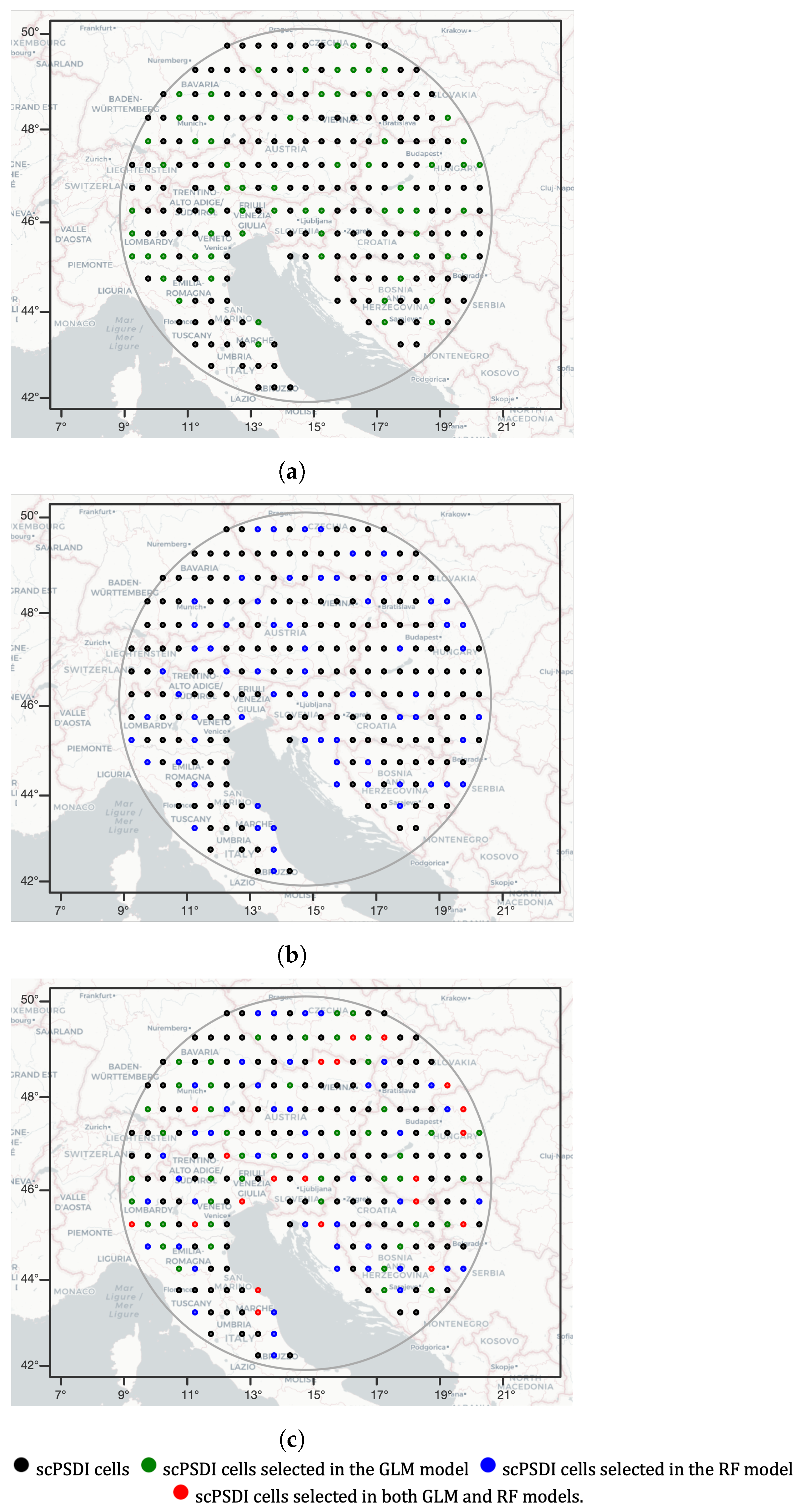
• A set of 249 self-calibrated Palmer Drought Severity Index (scPDSI) cells located within a 450 km radius of the SRB and a portion of the Old Water Drought Atlas (OWDA) developed from summer-related tree-ring proxies over a period from year 0 to 2012 were used [19]. This index has been shown to have significant and positive correlations with SR water flux, making it a valuable proxy for streamflow reconstructions in SRB [13].
• The reconstructed alpine monthly precipitation dataset, also known as the Long-term Alpine Precipitation Reconstruction (LAPrec), is derived from in situ observations. This dataset provides gridded fields of monthly precipitation for the Alpine region, covering eight countries. It has been meticulously constructed to meet high climatological standards, ensuring temporal consistency and the realistic reproduction of spatial patterns over complex terrains. The dataset spans from 1871 to 2020 and boasts a horizontal resolution of 5 km [20]. LAPrec combines two primary data sources:

  –

  Historical Instrumental Climatological Surface Time Series of the Greater Alpine Region (HISTALP) offers homogenized station series of monthly precipitation that date back to the 19th century. This version of the dataset, which starts in 1871, uses 85 almost-continuous series that are uniformly distributed across the Alpine region [20].

  –

  Alpine Precipitation Grid Dataset (APGD) provides daily precipitation gridded data for the period 1971–2008 constructed from more than 8500 rain gauges. This dataset incorporates daily precipitation measurements from over 5500 rain gauges on average per day, covering the entire Alpine region and ensuring a dense in situ observation network over high-alpine topography [20].

• The LAPrec dataset was developed using the Reduced Space Optimal Interpolation (RSOI) method, which establishes a linear model between station and grid data. This method involves Principal Component Analysis (PCA) of the high-resolution grid data followed by Optimal Interpolation (OI) using the long-term station data. The dataset was developed as a collaboration between the national meteorological services of Switzerland (MeteoSwiss, Federal Office of Meteorology and Climatology) and Austria (ZAMG, Zentralanstalt für Meteorologie und Geodynamik).
• It is important to note that climate conditions have been changing through the decades, and the selection of the dataset can impact the results. However, the dataset chosen for this study was constructed using state-of-the-art climatological approaches, ensuring a homogeneous dataset that adheres to the standards set by European meteorological offices.
• For this study, the SRB catchment average monthly precipitation was extracted based on the gridded precipitation data, with a focus on the seasonal April–May–June–July–August–September (AMJJAS) period.

The techniques used to perform the SRB AMJJAS precipitation reconstruction are divided into two groups. The first consists of nine “General Machine Learning Models” that use cross-validation techniques to evaluate their performance. The second group, referred to in this study as “Specialized Machine Learning Models”, consists of optimized or more advanced DL models. In both groups, the AMJJAS precipitation data accumulated between the months of April and September (AMJJAS) for the period from 1876 to 2012 were used as the dependent variable (label), while the 249 scPSDI cells were used as independent variables (features).

2.1. Metrics

Three key metrics were utilized in this study to evaluate the effectiveness of the models: Root Mean Square Error (RMSE), Nash–Sutcliffe Efficiency (NSE), and Kling–Gupta Efficiency (KGE). To ensure robustness and prevent overfitting, these metrics were computed using the validation datasets.

Root Mean Square Error (RMSE), a popular regression analysis statistic, determines the average size of errors between predicted and observed values. The RMSE is useful in scenarios where significant errors are undesirable. It is particularly sensitive to outliers and gives greater weight to larger errors. Nonetheless, its lack of normalization can sometimes impede comparison with other datasets or models [21].

Nash–Sutcliffe Efficiency (NSE), developed by Nash and Sutcliffe in 1970, is commonly applied in hydrology to assess the predictive accuracy of hydrological models. The normalized value provides ranges between $-\infty$ and 1, facilitating straightforward comparisons between different models. However, the calculation is unable to produce values for instances where the observed variance is zero, and it has a particular sensitivity to extreme values [22,23].

Kling–Gupta Efficiency (KGE) performs a comprehensive evaluation of hydrological models. It considers various aspects of the model’s predictions, including correlation, bias, and variability. Developed as a multi-objective function that offers a comprehensive view of model performance, KGE requires more computational resources than single-objective metrics [23,24].

The study posits that these three metrics deliver unique perspectives on various aspects of model performance, each with benefits and drawbacks. By collectively considering these principles, the objective is to present a comprehensive and refined understanding of the model’s predictive ability, ensuring that no performance aspect is disregarded.

2.2. General Machine Learning Models

The ML models tested are diverse and cover a wide range of techniques and approaches. Linear Regression (LR) is a statistical model that examines the linear relationship between two or more variables, with a dependent variable and one or more independent variables. Alternatively, Support Vector Machine (SVM) is a supervised learning model that uses classification algorithms to find a hyperplane that best divides a dataset into classes. Deep Learning (DL) refers to neural networks with three or more layers that attempt to simulate the behavior of the human brain to “learn” from large amounts of data. The Generalized Linear Model (GLM) extends the General Linear Model by allowing the amount of variance of each observation to depend on its predictive value. The k-Nearest Neighbors (kNN) algorithm allows prediction of both discrete and continuous values based on a measure of similarity between all available cases. Gradient Boosted Trees (GBT) is a machine learning technique that builds a predictive model in the form of a set of decision trees. Decision Trees (DTs) are supervised learning models primarily used for classification problems but that can also be effective in regression by predicting continuous values instead of class labels. Random Forest (RF) is an ensemble learning method that works by constructing multiple decision trees during training. Finally, the Gaussian Process (GP) is a nonparametric probabilistic model used in machine learning for regression and classification [25,26,27,28].

The performance of these nine ML models was evaluated using 10-fold cross-validation, with RMSE, NSE, and KGE as the metrics. Based on the initial evaluation, the GLM and RF models displayed the best performance. As a result, an automated feature-engineering process was applied specifically to these two models to test all possible feature subsets to determine the optimal combination of scPDSI cells that contributed the most. This process was performed with a balance for accuracy of 0.9 and optimization heuristics. Subsequently, reconstructions were generated for both the GLM and RF models using the full 249-feature dataset as well as the reduced feature-identified datasets covering the entire study period from year 0 to 2012.

A limitation of this regression modeling approach is that time is not considered as a factor during model training, which can adversely affect model performance in time-sensitive predictions. To mitigate this limitation, we included a 10-year time window in the GLM and RF models to extract sequential information from the dataset. The next year’s precipitation was used as the ground truth for each window, and the step size was one year, resulting in a total of 127 windows. Relying on this time-based analysis, reconstructions were performed for the entire dataset and for the reduced-feature-identified datasets for the period from year 10 to 2012.

2.3. Specialized Machine Learning Models

Two specialized machine learning models were implemented. The first consists of a deep learning neural network with three hidden layers of 500, 100, and 50 neurons, respectively. This network uses the Rectifier Linear Unit (ReLU) activation function. To optimize the training, the ADADELTA method was used, which combines the advantages of slowing down the learning rate with impulse-based training, thus avoiding slow convergence [29]. Although the loss function was determined automatically, the training was limited to 40 epochs. However, an early termination condition with a tolerance of 0.001 was included to avoid overfitting. For training and validation, the dataset was divided into 70% for training and 30% for validation. This training process was repeated 2000 times, with the best performing model selected at the end.

For the second model, the information from the scPDSI cells was normalized and consolidated into a single collection. Subsequently, this collection was transformed into tensors to perform a time-series analysis. A deep neural network integrating a Long Short-Term Memory (LSTM) layer with the ReLU activation function followed by a recurrent output layer—also with ReLU activation but using Mean Squared Error (MSE) as a loss function—was employed. The training process was spread over 122 epochs and had a batch size of eight examples. Optimization by stochastic gradient descent and standard backpropagation was employed; the learning rate was set to 0.01 and bias initialization to 0.1. To update the weights and bias values in the network, the Adam optimization method, which facilitates an adaptive change of momentum, was used [30].

As with the General Machine Learning models, the reconstructions derived from these specialized models covered the entire study period from year 0 to 2012, ensuring a consistent and comparable evaluation over the entire time period.

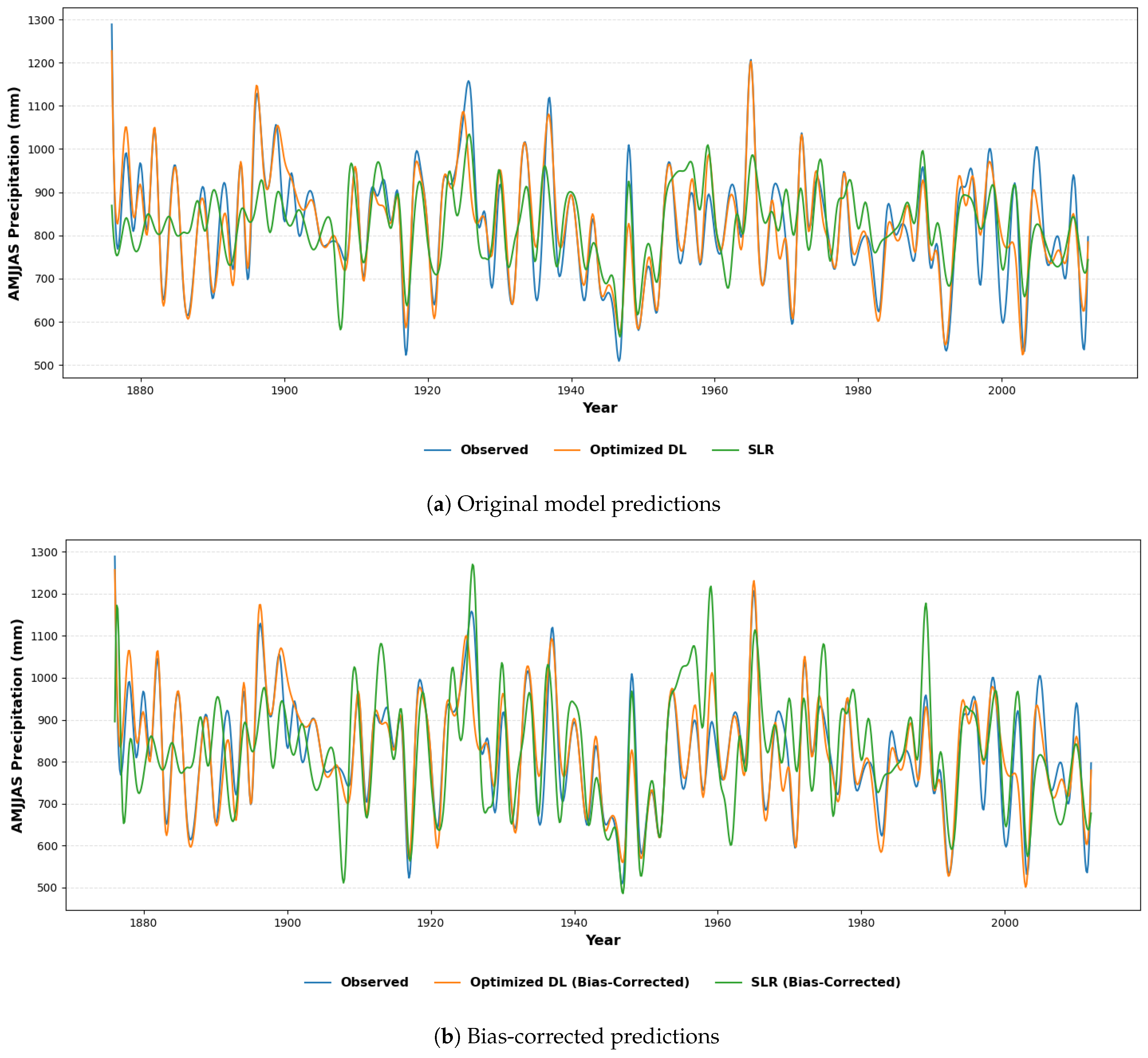
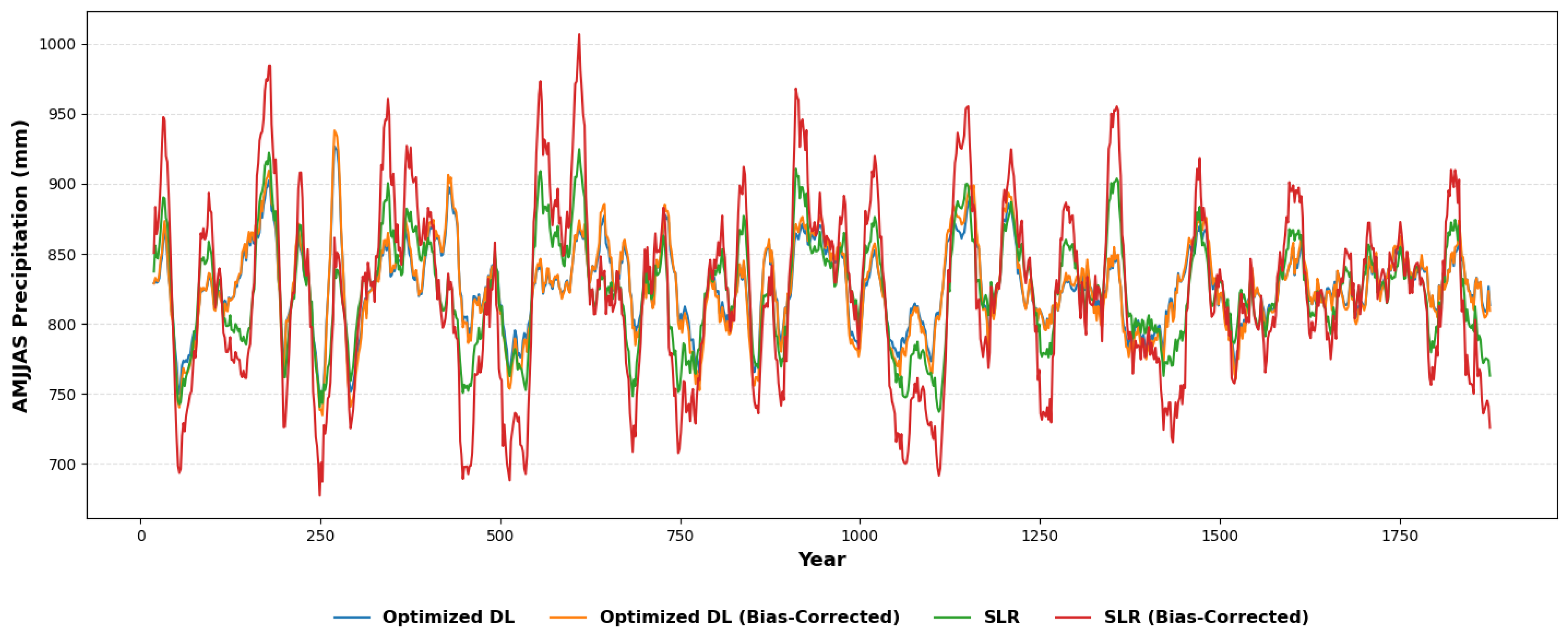
2.4. Bias Correction

To increase the reliability of the reconstructions, bias correction was applied using the quantile mapping method “RQUANT” as implemented in the qmap library [31] in R [32]. This nonparametric approach uses local, linear regressions on sequences of regularly spaced quantiles to approximate the quantile–quantile relationship. The main advantage of RQUANT is its ability to closely match the observed and modeled cumulative distribution functions (CDF) without overfitting. It provides a more flexible and robust correction compared to parametric methods, which often assume an underlying distribution and may not account for variations in bias across the empirical CDF. In this study, the statistical properties of the reconstruction are assumed to remain constant over time. This suggests that any bias present in the data during the observation period is expected to be analogous to the bias in the reconstructed data from earlier times [33]. This bias correction method is consistent with the approach used in [5] and ensures comparability of the results.

3. Results

The performance of the nine General Machine Learning models, as evaluated through cross-validation, is summarized in

Table 1. General Machine Learning Models’ performance.

Model	RMSE	NSE	KGE
Linear Regression (LR)	230.890	0.233	0.339
Support Vector Machine (SVM)	128.060	0.252	0.425
Deep Learning (DL)	138.517	0.161	0.281
Generalized Linear Model (GLM)	116.070	0.281	0.408
k-Nearest Neighbors (kNN)	122.142	0.217	0.358
Gradient Boosted Trees (GBT)	125.479	0.187	0.353
Decision Tree (DT)	141.717	0.201	0.385
Random Forest (RF)	119.210	0.265	0.405
Gaussian Process (GP)	835.935	0.064	−4.137

. In particular, the GLM and RF models demonstrated superior accuracy, both achieving an RMSE below 120 mm, an NSE above 0.25, and a KGE above 0.4. Given their performance, these two models were selected for further analysis.

During the automated feature engineering phase, several scPDSI cells emerged as significant contributors to the models. The GLM model included 67 of these cells, while the RF model used 66. Of these, 21 cells were consistently selected by both models, highlighting their importance in the SRB precipitation reconstruction. The spatial distribution of these cells can be visualized in Figure 2.

Feature engineering had a mixed effect on the performance of the models. For the GLM model, there was an improvement in performance, while for the RF model, there was a slight decrease in performance.

Table 2. Selected General Machine Learning Models’ performance before and after automated feature engineering.

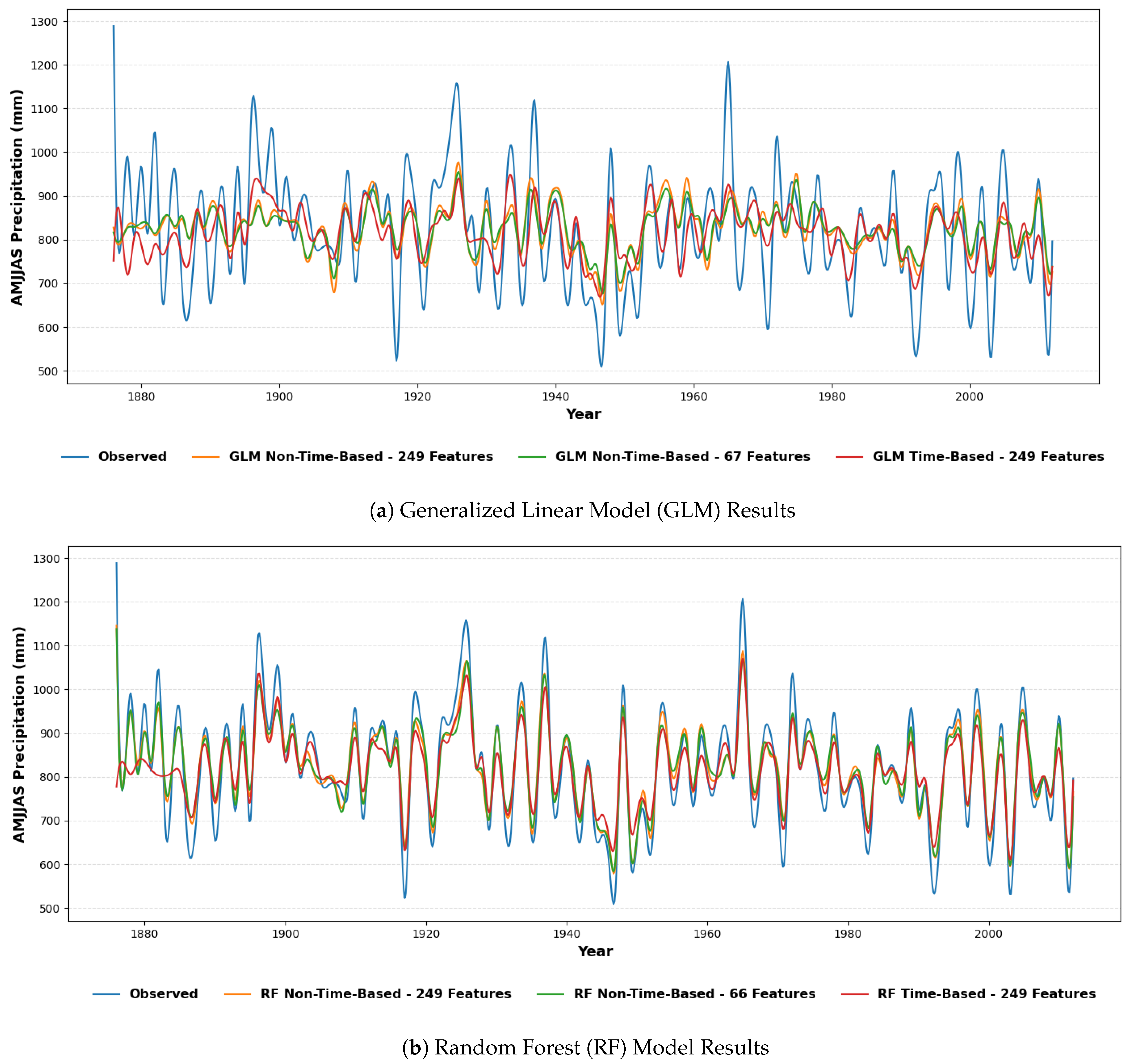
Model	Entire Data Set (249 Features)			Reduced-Feature Datasets (67 Features for GLM and 66 for RF)
	RMSE	NSE	KGE	RMSE	NSE	KGE
Generalized Linear Model (GLM)	116.070	0.281	0.408	115.631	0.327	0.447
Random Forest (RF)	119.210	0.265	0.405	120.226	0.251	0.378

shows the RMSE, NSE and KGE values before and after feature engineering for both models. This behavior can be explained by the fact that GLM, being a linear model that benefits from feature selection because it reduces multicollinearity and improves model interpretation by reducing irrelevant or redundant features, allows the model to focus on the most significant linear relationships between the features and the target variable. RF, on the other hand, is a model that can handle a large number of features and automatically determine the importance of each feature. Therefore, by reducing the number of features, it is possible that some information that the model could have used to make splits in the trees is eliminated [25,34].

As mentioned above, the time-based analysis process implemented a 10-year moving window, which resulted in multiplying the features by a factor of 10. The purpose of this analysis was to use the information from the preceding 10 years to predict the present.

Table 3. GLM and RF performance under different scenarios.

Model	Non-Time-Based Analysis		Time-Based Analysis
	RMSE (Whole Feature Set)	RMSE (Post-Feature Engineering)	RMSE (Whole Feature Set)	RMSE (Post-Feature Engineering)
Generalized Linear Model (GLM)	116.070	115.631	133.328	133.694
Random Forest (RF)	119.210	120.226	133.211	132.975

shows the RMSE for the GLM and RF models under different scenarios: non-time-based analysis, post-feature engineering, and time-based analysis. NSE and KGE metrics are not included because increasing the number of features artificially distorts the calculation. Although feature engineering showed a marginal improvement in performance for the non-time-based analysis of the GLM model, it is noteworthy that the time-based analysis led to a decline in performance, which can be seen in Figure 3. Despite the use of cross-validation, the increased complexity of the model due to the larger number of features may have led to overfitting in the training data. This may explain the decline in performance observed in the test data for each fold during the time-based analysis.

After evaluating the performance of the General Machine Learning models, the specialized models were analyzed, which, as anticipated in the methodology, incorporate optimized Deep Learning techniques.

Table 4. Specialized Machine Learning Models’ performance on the test data.

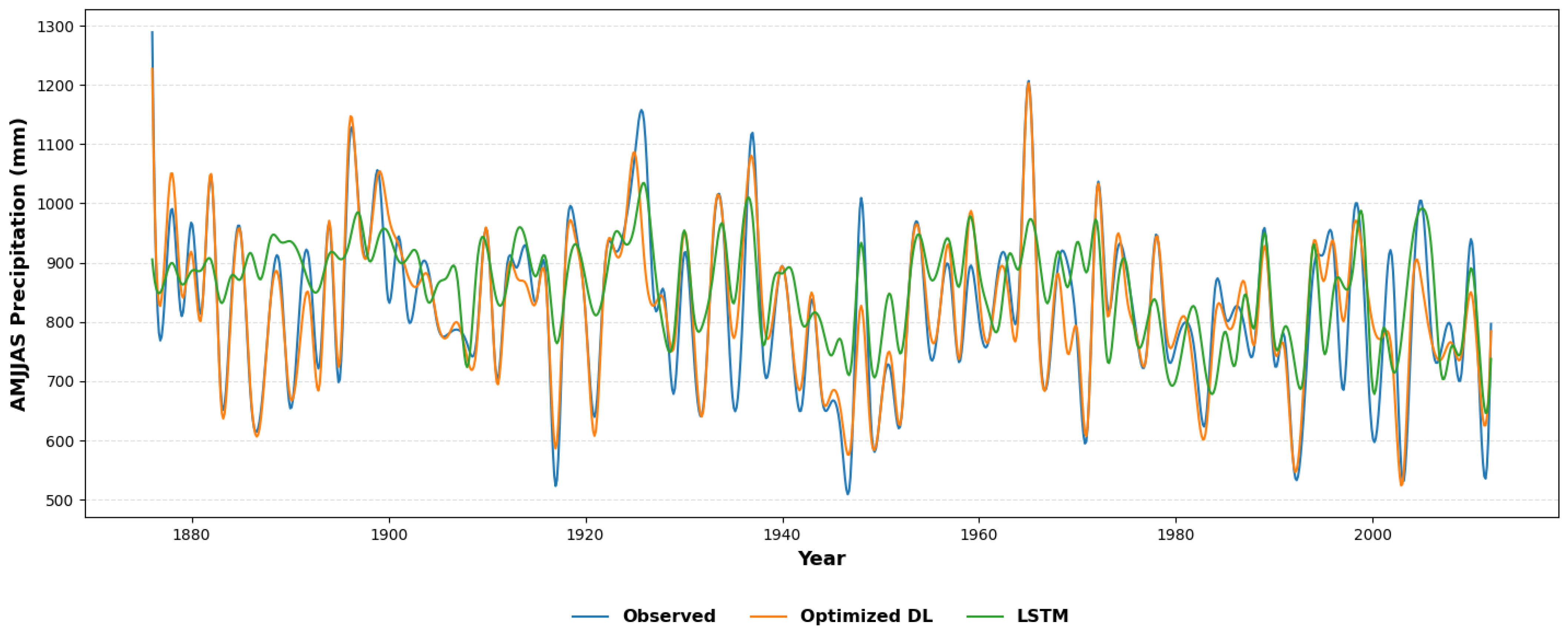
Model	RMSE	NSE	KGE
Optimized Deep Learning (Optimized DL)	89.225	0.367	0.468
Long Short-Term Memory (LSTM)	109.005	0.150	0.580

shows the performance of the two implemented specialized models. It is noteworthy that both models outperformed all the general models, with the optimized deep learning model, called Optimized DL, obtaining the lowest error when applied to the test data compared to the LSTM-based model.

Figure 4 shows a comparison between the predictions of the specialized models and the observed data. The Optimized DL model closely follows the trend of the observed data. The LSTM-based model, while also matching the trend, was not as accurate in predicting the extreme values. This discrepancy may be due to the inherent nature of LSTM networks, which are designed to remember patterns over long sequences [35]. Given the oscillatory nature of the observed data, with significant year-to-year variations, the LSTM may struggle to accurately capture these rapid changes. In addition, it may sometimes smooth or average extreme values, especially if such extremes are not consistently present in the training data or are considered outliers. This behavior may result in the LSTM model not emphasizing rare or atypical peaks and troughs as much as models such as Optimized DL.

4. Discussion

Since the Optimized DL model outperformed all other evaluated models, bias correction was applied to its results. Subsequently, its performance was compared with the results obtained with the Stepwise Linear Regression (SLR) model used in [5]. For a fair comparison with the SLR method, the RMSE, NSE, and KGE metrics were calculated over the entire dataset. As can be seen in

Table 5. Performance comparison between the predictions of the Optimized DL model and the SLR model.

Model	Original Model Predictions			Bias-Corrected Predictions
	RMSE	NSE	KGE	RMSE	NSE	KGE
Optimized Deep Learning (Optimized DL)	52.207	0.852	0.891	53.632	0.844	0.922
Stepwise Linear Regression (SLR)	107.257	0.377	0.454	119.833	0.223	0.611

, the Optimized DL model outperformed the SLR model in all metrics, both for the original model predictions and for those with bias correction. This improved performance is evident in Figure 5, where the results of the Optimized DL model, both with the original predictions and with the bias correction, are closer to the observed values.

Consequently, the Optimized DL model was applied to the scPDSI cell data for the period from year 0 to 1875 to create the paleo-reconstruction of precipitation in the SRB. A comparison between this paleo-reconstruction and the SLR model is shown in Figure 6. To visualize these results, a 20-year end-year filter was implemented to smooth the curve in order to focus more on the general trend than on the annual variations.

A similarity in precipitation amounts between the original reconstruction and the bias correction is observed when looking at the reconstruction performed by the Optimized DL model. This similarity can be attributed to the high prediction performance of this model, where its estimates are remarkably close to the observed values. As a result, it is plausible that the predictions for the paleo-reconstruction period, for which no observed data exist, are well-calibrated and thus require minimal bias correction.

A comparison of the SLR and Optimized DL model reconstructions shows that although the overall trend direction is similar in both models, the precipitation magnitudes estimated by the SLR model are generally larger than those of the Optimized DL model. This discrepancy in magnitude can be attributed to inherent differences in how these models process and fit the data. The SLR model, being a linear model, may capture general trends and consequently overestimate certain magnitudes based on the linear relationship identified. In contrast, the Optimized DL model, being a more sophisticated model, can identify and fit more complex non-linear relationships and patterns in the data, which could result in more accurate and nuanced predictions.

The Optimized DL Bias-Corrected Reconstructed AMJJAS annual (0 to 1900) precipitation developed in this research and the SLR Bias-Corrected Reconstructed AMJJAS annual (0 to 1900) streamflow developed in [5] were standardized (mean of zero and standard deviation of one), and the annual values were highly correlated (r = 0.59/>99.9% significance). This indicates that despite the use of two different reconstruction techniques (Optimized DL and SLR) and two different hydrologic datasets (precipitation and streamflow), the overall temporal behavior was similar. Given the differences in magnitude between AMJJAS streamflow and AMJJAS precipitation, the standardization of these datasets allows for easier comparison. A 20-year filter was applied to both datasets to visually examine similarities and differences in drought and pluvial periods (Figure 7). The two highest AMJJAS streamflow (blue line) pluvial events (~610 AD and ~1136 AD) were not identified (captured) with the AMJJAS precipitation reconstruction (orange line). Similarly, the highest AMJJAS precipitation (blue line) pluvial event (~270 AD) was not identified (captured) with the AMJJAS streamflow reconstruction (red line). Thus, while the temporal variability of the two datasets was statistically similar, we identified differences in pluvial magnitudes for the most extreme events (years). Drought extremes provided a different result (visual observation), as ~53 AD and ~253 AD were identified in both streamflow and precipitation. Per a visual inspection of Figure 7, drought “agreement”, both in timing (temporal variability) and magnitude, appears more consistent than when visually inspecting and evaluating pluvial periods. Thus, we conclude that we have greater confidence (less uncertainty) in identifying SRB droughts when using tree-ring-based proxies.

5. Conclusions

The Optimized DL model has proven to be a robust tool in reconstructing precipitation patterns, outperforming conventional linear models such as the SLR. Its inherent ability to discern intricate non-linear relationships within datasets facilitates more accurate projections, particularly when contrasted with linear models that might exaggerate certain magnitudes based on detected linear relationships.

The integration of the Optimized DL model with the scPDSI cell data has enabled a meticulous paleo-reconstruction of precipitation in the SRB, providing insight into historical rainfall patterns and their implications. This perspective becomes especially relevant in the context of challenges posed by climate change and the pressing need for precise ancient climatic records to underpin future projections and shape strategies.

Although both the Optimized DL model and the SLR exhibited analogous temporal dynamics in their reconstructions, discrepancies in the magnitudes of extreme rainfall events were palpable. However, the consistency in drought event detection indicates that proxies derived from tree rings constitute a reliable method for identifying droughts in the SRB. This highlights the importance of combining conventional climatic indicators with cutting-edge modeling techniques to achieve a more comprehensive interpretation of past climatic phenomena.

Additionally, the significant correlation between the standardized annual values of the reconstructed annual precipitation AMJJAS with bias correction from Optimized DL and the reconstructed annual flow AMJJAS with SLR bias correction emphasizes the feasibility of integrating various hydrological datasets to strengthen reconstructions.

The implementation of advanced machine learning models emerges as a promising route to enhance the accuracy and reliability of hydroclimatological reconstructions, especially in areas with intricate climatic patterns. As hydrology continues to evolve, the incorporation of these novel techniques becomes essential to sharpen our understanding of past, present, and forthcoming hydroclimatic patterns.

References

- Leščešen, I.; Šraj, M.; Basarin, B.; Pavić, D.; Mesaroš, M.; Mudelsee, M. Regional Flood Frequency Analysis of the Sava River in South-Eastern Europe. Sustainability 2022, 14, 9282. [Google Scholar]
- Brilly, M. (Ed.) Hydrological Processes of the Danube River Basin: Perspectives from the Danubian Countries; Springer: Dordrecht, The Netherlands, 2010. [Google Scholar] [CrossRef]
- Bezak, N.; Horvat, A.; Šraj, M. Analysis of flood events in Slovenian streams. J. Hydrol. Hydromech. 2015, 63, 134–144. [Google Scholar] [CrossRef][Green Version]
- Frantar, P.; Hrvatin, M. Pretočni režimi v Sloveniji med letoma 1971 in 2000. Geogr. Vestn. 2005, 77, 115–127. [Google Scholar]
- Tootle, G.; Oubeidillah, A.; Elliott, E.; Formetta, G.; Bezak, N. Streamflow Reconstructions Using Tree-Ring-Based Paleo Proxies for the Sava River Basin (Slovenia). Hydrology 2023, 10, 138. [Google Scholar] [CrossRef]
- Vrzel, J.; Solomon, D.K.; Blažeka, Ž.; Ogrinc, N. The study of the interactions between groundwater and Sava River water in the Ljubljansko polje aquifer system (Slovenia). J. Hydrol. 2018, 556, 384–396. [Google Scholar] [CrossRef]
- Copernicus Emergency Management Service. Flood in Slovenia: EMSR680-Situational reporting. EGUsphere 2023, 2023, 1–13. [Google Scholar]
- Agencija Republike Slovenije za Okolje—ARSO. Nalivi in obilne padavine od 3. do 6. avgusta 2023. Ministrstvo za Okolje, Podnebje in Energijo. 2023. Available online: https://meteo.arso.gov.si/uploads/probase/www/climate/text/sl/weather_events/padavine_3-6avg2023.pdf (accessed on 10 September 2023).
- Steinhausen, M.; Paprotny, D.; Dottori, F.; Sairam, N.; Mentaschi, L.; Alfieri, L.; Lüdtke, S.; Kreibich, H.; Schröter, K. Drivers of future fluvial flood risk change for residential buildings in Europe. Glob. Environ. Chang. 2022, 76, 102559. [Google Scholar] [CrossRef]
- Zalokar, L.; Kobold, M.; Šraj, M. Investigation of Spatial and Temporal Variability of Hydrological Drought in Slovenia Using the Standardised Streamflow Index (SSI). Water 2021, 13, 3197. [Google Scholar] [CrossRef]
- Predin, A.; Fike, M.; Pezdevšek, M.; Hren, G. Lost Energy of Water Spilled over Hydropower Dams. Sustainability 2021, 13, 9119. [Google Scholar] [CrossRef]
- Trček, B.; Mesarec, B. Impact of the Hydroelectric Dam on Aquifer Recharge Processes in the Krško Field and the Vrbina Area: Evidence from Hydrogen and Oxygen Isotopes. Water 2023, 15, 412. [Google Scholar] [CrossRef]
- Trlin, D.; Mikac, S.; Žmegač, A.; Orešković, M. Dendrohydrological Reconstructions Based on Tree-Ring Width (TRW) Chronologies of Narrow-Leaved Ash in the Sava River Basin (Croatia). Sustainability 2021, 13, 2408. [Google Scholar] [CrossRef]
- Ho, M.; Lall, U.; Cook, E.R. Can a paleodrought record be used to reconstruct streamflow?: A case study for the Missouri River Basin. Water Resour. Res. 2016, 52, 5195–5212. [Google Scholar] [CrossRef]
- Ho, M.; Lall, U.; Sun, X.; Cook, E.R. Multiscale temporal variability and regional patterns in 555 years of conterminous US streamflow. Water Resour. Res. 2017, 53, 3047–3066. [Google Scholar] [CrossRef]
- Formetta, G.; Tootle, G.; Bertoldi, G. Streamflow Reconstructions Using Tree-Ring Based Paleo Proxies for the Upper Adige River Basin (Italy). Hydrology 2022, 9, 8. [Google Scholar] [CrossRef]
- Formetta, G.; Tootle, G.; Therrell, M. Regional Reconstruction of Po River Basin (Italy) Streamflow. Hydrology 2022, 9, 163. [Google Scholar] [CrossRef]
- Isaev, E.; Ermanova, M.; Sidle, R.C.; Zaginaev, V.; Kulikov, M.; Chontoev, D. Reconstruction of Hydrometeorological Data Using Dendrochronology and Machine Learning Approaches to Bias-Correct Climate Models in Northern Tien Shan, Kyrgyzstan. Water 2022, 14, 2297. [Google Scholar] [CrossRef]
- Cook, E.R.; Seager, R.; Kushnir, Y.; Briffa, K.R.; Büntgen, U.; Frank, D.; Krusic, P.J.; Tegel, W.; van der Schrier, G.; Andreu-Hayles, L.; et al. Old World megadroughts and pluvials during the Common Era. Sci. Adv. 2015, 1, e1500561. [Google Scholar] [CrossRef] [PubMed]
- Climate Change Service. Alpine Gridded Monthly Precipitation Data Since 1871 Derived from In-Situ Observations. 2021. Available online: https://cds.climate.copernicus.eu/cdsapp#!/dataset/10.24381/cds.6a6d1bc3?tab=overview (accessed on 28 August 2023).
- Hyndman, R.J.; Koehler, A.B. Another look at measures of forecast accuracy. Int. J. Forecast. 2006, 22, 679–688. [Google Scholar] [CrossRef]
- Nash, J.; Sutcliffe, J. River flow forecasting through conceptual models part I—A discussion of principles. J. Hydrol. 1970, 10, 282–290. [Google Scholar] [CrossRef]
- Knoben, W.J.M.; Freer, J.E.; Woods, R.A. Technical note: Inherent benchmark or not? Comparing Nash–Sutcliffe and Kling–Gupta efficiency scores. Hydrol. Earth Syst. Sci. 2019, 23, 4323–4331. [Google Scholar] [CrossRef]
- Gupta, H.V.; Kling, H.; Yilmaz, K.K.; Martinez, G.F. Decomposition of the mean squared error and NSE performance criteria: Implications for improving hydrological modelling. J. Hydrol. 2009, 377, 80–91. [Google Scholar] [CrossRef]
- Skiena, S.S. The Data Science Design Manual, 1st ed.; Texts in Computer Science; Springer: Cham, Switzerland, 2017. [Google Scholar] [CrossRef]
- Deisenroth, M.P.; Faisal, A.A.; Ong, C.S. Mathematics for Machine Learning; Cambridge University Press: Cambridge, UK, 2020. [Google Scholar] [CrossRef]
- Bonaccorso, G. Machine Learning Algorithms, 2nd ed.; Packt: Birmingham, UK, 2018; p. 522. [Google Scholar]
- RapidMiner Inc. RapidMiner Documentation-Operators. 2023. Available online: https://docs.rapidminer.com/latest/studio/operators/ (accessed on 29 June 2023).
- Zeiler, M.D. ADADELTA: An Adaptive Learning Rate Method. arXiv 2012, arXiv:1212.5701. [Google Scholar]
- Kingma, D.P.; Ba, J. Adam: A Method for Stochastic Optimization. arXiv 2017, arXiv:1412.6980v9. [Google Scholar]
- Gudmundsson, L.; Bremnes, J.B.; Haugen, J.E.; Engen-Skaugen, T. Technical Note: Downscaling RCM precipitation to the station scale using statistical transformations—A comparison of methods. Hydrol. Earth Syst. Sci. 2012, 16, 3383–3390. [Google Scholar] [CrossRef]
- RC Team. A Language and Environment for Statistical Computing; R Foundation for Statistical Computing: Vienna, Austria, 2018; Available online: https://www.R-project.org/ (accessed on 11 September 2023).
- Robeson, S.M.; Maxwell, J.T.; Ficklin, D.L. Bias Correction of Paleoclimatic Reconstructions: A New Look at 1200+ Years of Upper Colorado River Flow. Geophys. Res. Lett. 2020, 47, e2019GL086689. [Google Scholar] [CrossRef]
- Wang, K.; Wang, P.; Xu, C. Toward Efficient Automated Feature Engineering. In Proceedings of the 2023 IEEE 39th International Conference on Data Engineering (ICDE), Anaheim, CA, USA, 3–7 April 2023; pp. 1625–1637. [Google Scholar] [CrossRef]
- Hochreiter, S.; Schmidhuber, J. Long Short-Term Memory. Neural Comput. 1997, 9, 1735–1780. [Google Scholar] [CrossRef]