Abstract
Over the past century, increases in indigenous woody plant species, also known as woody encroachment (WE), has occurred in grasslands and savannas across the globe. While the impact on grassland and savanna composition and productivity has been well studied, little is known of the impacts on the hydrological cycle. WE may increase evapotranspiration (ET) losses, leading to reduced infiltration and ultimately reduced freshwater availability, which is of particular concern in arid and semi-arid areas. The aim of this study was to determine the effect of Colophospermum mopane (mopane) encroachment on ET in a semi-arid savanna located in South Africa. Mopane is widely distributed across southern Africa, and is one of the main encroaching species of the region. Following an assessment of the validity of two surface renewal approaches, SR1 and SRDT, against short eddy covariance campaigns for sensible heat flux estimation, the SR1 approach was used to estimate ET at an experimental woody plant clearing trial from November 2019 to July 2022. For the two drier years of the study, the removal of mopane trees had little effect on ET. However, for the wettest year of the study, the removal of mopane trees decreased ET by 12%, supporting the hypothesis that the conversion from grass dominance to woody dominance can increase ET. Annual ET exceeded annual rainfall in all 3 years, indicating that the vegetation supplements its water use with soil water that has accumulated during previous wet seasons, or that tree roots facilitate hydraulic lift of deep soil water, or groundwater, to depths within the rooting depth of both trees and grasses. Further research is needed to confirm the exact mechanism involved, and the consequences of this for groundwater and streamflow at landscape scales.
1. Introduction
Increases in the density and cover of indigenous woody plants at the expense of the grass layer, a phenomenon termed woody encroachment (WE), has occurred in grasslands and savannas across the globe over the past century, and is still occurring in many areas [1,2]. For decades, debate has surrounded the causes of WE, with varying degrees of evidence for overgrazing, a loss of browser herbivores, fire suppression, warmer temperatures, altered rainfall patterns and increasing atmospheric CO2 concentrations being responsible [3]. In southern Africa, WE has been particularly widespread in arid and semi-arid savannas, with as much as 20 million hectares affected in South Africa alone [4]. These savannas typically have and low total precipitation coupled with high seasonal variability [5], and water is a key limitation on ecosystem productivity and economic development. There is growing concern that WE may escalate the risk of water shortages by increasing evapotranspiration (ET) losses, as woody plants are typically taller, have larger leaf areas, longer growing periods and deeper roots compared to the grasses they replace. Therefore, with increased woody densities, less water will be available in the system to supply stormflow and baseflow for streams and/or groundwater stores [6,7].
One of the dominant encroacher tree species in the semi-arid savannas of South Africa is Colophospermum mopane (Kirk ex Benth) Kirk éx J. Léonard (mopane) [8]. Mopane is considered to be an aggressive competitor for available soil water with shallow-rooted grasses and other woody plants because it tends to grow in dense, monotypic stands with little to no grass cover [9,10]. Mopane’s competitive advantage for water is largely attributed to the structural, physical and physiological adaptations of its roots and leaves, which at the same time allow it to survive in extremely dry conditions [9,11]. Although the roots of mopane are not as deep as other trees, the species has a large root biomass which extends horizontally well beyond the extent of its canopy [9,12], allowing access to soil water over a large area. Mopane roots can also extract water when soils are very dry as they have the ability to utilize soil water at lower matric water potentials than those tolerated by grasses and other woody plants [13]. The leaves of mopane are compound and compose of two ovate leaflets, which have the ability to fold together during hot periods to limit transpiration [11]. Mopane is deciduous and limits its transpiration during the dry winter season by shedding its leaves, but typically retains its leaves longer into the dry season than co-occurring woody species and grasses [10,11].
The effect of WE by mopane on ET is yet to be established. In fact, few studies have measured changes in ET in response to any encroaching species anywhere in Africa. Theory and ecohydrological models predict that WE can increase ET losses in mesic environments because high rainfall allows the potential for high transpiration and interception rates [6,14]. In arid environments, Huxman et al. [6] reported that WE has less of an effect on ET because most precipitation is evaporated irrespective of the type of vegetation, whereas Schreier-McGraw et al. [14] predicted that WE decreases ET, due to a reduction of infiltration caused by increases in bare soil cover. While several international studies have found evidence that WE increased ET losses in semi-arid savanna vegetation types [15,16,17], similar studies are needed from southern African systems to confirm that these results can be generalized to the region.
A variety of micrometeorological methods are available for field-scale ET estimation, including eddy covariance (EC), large weighing lysimeters, optical scintillation and the Bowen ratio energy balance (BREB) method [18]. However, the expense of the sophisticated instrumentation required by most of these methods, as well as a shortage of experienced technicians equipped with the necessary skills to setup and operate the equipment, has hindered their use in the developing southern African region [19,20,21]. The method considered to be most universally accurate is EC [22]. EC directly calculates latent heat flux (LE) (and ET) as the covariance between turbulent fluctuations of vertical wind speed and water vapor exchange between the atmosphere and plant canopy [23]. In addition to the high-cost, continuous maintenance and complex operation of EC, a number of issues have prevented its widespread use [23,24]. EC sensors require installation in the inertial sublayer above the roughness sublayer, which is generally estimated as twice the canopy height. The higher the sensor is installed, the larger the area of fetch (i.e., upwind distance from the sensor with uniform features) required to achieve representative measurements for the vegetation of interest. Therefore, the use of EC is limited in small experimental plots, and a lack of fetch is a common reason why energy balance closure from EC measurements is not accomplished [25,26]. Furthermore, EC sensors are sensitive and their accuracy can be affected by terrain properties, sensor positioning and alignment, low wind speeds and unfavorable wind directions [24,26].
In recent years, simpler alternative methods for estimating ET that overcome the shortcomings of EC have been sought. One of these methods that has drawn attention in the literature is surface renewal (SR) [23]. While SR is not a new method, an increasing number of studies are reporting on its successful application for estimating ET over a wide range of surfaces, including water, bare soil, wetlands, grasses and a variety of agricultural crops [18]. SR has not yet been widely used in southern Africa, but to date, it has been successfully tested against EC, scintillometer and BREB measurements over a mesic grassland [27], an open water reservoir [28], a wetland [29], a Podocarpus falcatus plantation [30], a grassland encroached by Leucosidea sericea [21] and a grassland invaded by Pteridium aquilinium [31].
SR analysis, first introduced by Paw U et al. [32], is based on the turbulent exchange of sensible heat between the plant canopy and the atmosphere caused by the continuous exchange of air parcels [23]. High frequency air temperature readings collected above the vegetation canopy and the analysis of their ramp structures are used to estimate sensible heat flux (H). Thereafter, LE is calculated indirectly as the residual of the shortened surface energy balance equation, along with net radiation (Rn) and soil heat flux (G) measurements (i.e., LE = Rn − G − H) [33]. SR systems comprise of a simple design, requiring a minimum of one inexpensive fine-wire thermocouple, in addition to sensors for the measurements of Rn and G, which are also relatively inexpensive. The low-cost of the thermocouples not only makes it affordable to duplicate ET measurements in field experiments, but also allows for back-up sensors to be used, limiting data record gaps in the case of thermocouple damage [18,19,34,35]. The thermocouples and Rn and G sensors also have a low power consumption permitting fewer site visits [29]. All of these factors make SR a particularly useful method for long-term, unattended use in remote sites. Another significant attraction of SR is that a relatively small fetch is sufficient for reliable H measurements. Thermocouples capture very small eddies so a more localized process of H exchange can be examined, allowing for them to be deployed in the roughness sublayer, within or close to the canopy. This also makes SR a useful method at remote sites, because the measurement height does not have to be adjusted as the vegetation grows or dies back [26,36].
Several variations of the SR method exist [26]. SR1 [37] is the original, most documented and well tested SR approach. It is based on classical structure function analysis and only requires high frequency air temperature measurements for H estimation [19,35]. SR1 H estimates require site-specific calibration against a standard flux measurement method, such as EC. Calibration involves correcting H estimated with SR by means of a calibration factor (α), to account for uneven heating of air parcels below the thermocouple [25,35]. To avoid the dependency of SR on other methods, SR approaches exempt from calibration have been developed, including SR2 [34,38] and SRDT [39]. SR2 incorporates the principles of the Monin-Obukhov similarity theory (MOST) with structure function analysis [34]. In addition to high frequency air temperature measurements, SR2 requires horizontal wind speed measurements and specific flux parameters, such as zero-plane displacement height, roughness sub-layer depth and canopy parameters (i.e., leaf area index, canopy height and vertical extent of the foliage) to estimate H [19]. SRDT combines the Hsieh and Katul [40] dissipation method with structure function analysis and only requires air temperature measurements to estimate H [39]. Although the SRDT approach is the least tested approach, it has produced good H estimates over rangeland grass in California [39] and Leucosidea sericea and Pteridium aquilinium canopies in South Africa [21,31].
In this study, we used SR to determine the effect of mopane encroachment on ET in a semi-arid savanna ecosystem located in north-eastern South Africa. ET was measured continuously for 3 years from November 2019 to July 2022 at an experimental woody plant clearing trial. The validity of SR at the site was first tested by comparing two SR approaches, SR1 and SRDT, against the EC method. Thereafter, the SR approach which best agreed with EC, was used to estimate ET at two adjacent plots differing in woody plant density. To our knowledge, this is the first validation test of SR over semi-arid savanna-type vegetation worldwide.
2. Materials and Methods
2.1. Study Site
The study was carried out at the Mthimkhulu Game Reserve (MGR) (23°31′46″ S; 31°06′12″ E, elevation 335 m above sea level) in the Limpopo Province, South Africa (Figure 1). The MGR is owned by a local tribal authority but is part of the greater Kruger National Park, South Africa’s largest conservation area, and shares open borders with the north-eastern side of the park [41]. The vegetation of MGR is classified as Lowveld Mopaneveld [42,43], a semi-arid savanna characterized by a dense cover of mopane shrubs, sparsely scattered trees and a limited grass understory. According to a nearby rainfall station at Mahlangeni in the Kruger National Park, the area receives a mean annual precipitation (MAP) of 467 mm. Rainfall is highly seasonal, falling in the form of thunderstorms during the spring-summer months of October to March [43,44]. Temperatures are high in summer and mild in winter with a mean annual temperature of 21.6 °C [43,45]. The landscape is mostly flat and homogeneous with Goudplaats and Makhutswi Gneiss underlying shallow and well drained red-yellow apedal soils [43]. The seasonal Klein Letaba river, which is a tributary of the Letaba River, is situated adjacent to the site.
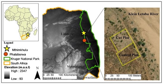
Figure 1.
Location of the Mthimkhulu Game Reserve in the Limpopo Province, north-eastern South Africa, and the location of the control and cut plots within the reserve.
The cover of mopane is extremely high in MGR, as well as surrounding areas, which is likely the result of WE that occurred in response to overgrazing by cattle over the past century. In 2014, the South African Environmental Observation Network (SAEON) established a long-term experimental woody plant clearing trial to determine the impact of mopane cover on ecosystem processes. This comprises of 5 ‘control’ plots and 5 neighbouring ‘cut’ plots, each approximately 3600 m2 in size. The control plots contain dense monotypic mopane stands with occasional Combretum imberbe and Vachellia tortilis and Combretum apiculatum and Grewia bicolor shrubs. The grass layer is sparse and consists mostly of annual Aristida species, with scattered tufts of Urochloa mosambicensis and Panicum maximum. The majority of the ground cover consists of bare soil and mopane leaf litter for much of the year. The cut plots were mechanically cleared of mopane trees by cutting all individuals shorter than four meters high, 1–2 times per year. No treatment has been applied to the control plots. For this study, one control plot and one neighbouring cut plot were selected for instrumentation and data collection (Figure 1). In this cut plot, the woody layer consisted of a few remaining mopane trees taller than 4 m, and the grass layer was a thick sward dominated by Urochloa mosambicensis. The soil of both plots was an alluvial soil more than 1 m deep (an Oakleaf soil form in the South African Soil Classification System [46]).
Identical SR systems were deployed at the control and cut plots from mid-November 2019 to mid-June 2022, as well as an Automatic Weather Station (AWS) at the cut plot. At each plot, two week-long EC field campaigns were carried out alongside the SR systems to determine α factors for SR1, and to test the validity of the SR1 and SRDT approaches for H estimation. The campaigns were conducted in different seasons, the first in the wet summer season (February 2020), and the second at the beginning of spring (October/November 2020) when conditions were drier (Figure 2).
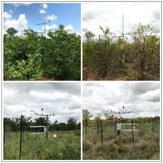
Figure 2.
Vegetation and research equipment at the control plot in the summer (top-left) and spring (top-right) campaigns, and the cut plot in the summer (bottom-left) and spring (bottom-right) campaigns.
2.2. Instrumentation
The AWS measured solar irradiance (CMP3, Kipp & Zonen, Delft, The Netherlands), air temperature and relative humidity (HMP60, Campbell Scientific Inc., Logan, UT, USA), wind speed and wind direction (Windsonic, Gill Instruments Ltd., Hampshire, UK) and rainfall (TR-525, Texas Electronics Inc., Dallas, TX, USA). All AWS sensors were installed on a tripod at 2 m above a short grass surface, except for the rain gauge, which was installed with its orifice at 1.2 m above the ground.
The SR systems each comprised of two unshielded 76 µm chromel-constantan fine-wire thermocouples (TCBR-3, Campbell Scientific Inc.) that measured high frequency air temperature at a sampling frequency of 10 Hz and at 0.4 s and 0.8 s time lags. The thermocouples were installed at 0.5 m and 1 m above the maximum expected canopy height (2.15 m and 0.55 m for the control and cut plots, respectively) and oriented toward the prevailing southerly wind direction to minimize wind distortion effects. Rn was measured with a net radiometer (NR Lite 2, Kipp and Zonen) installed 2 m above the ground and oriented toward the northerly direction. For G measurements, three soil heat flux plates (HFP01, Hukseflux Thermal Sensors, Delft, The Netherlands) were installed at a depth of 0.08 m, two soil temperature averaging soil thermocouple probes (TCAV, Campbell Scientific Inc.) were installed at depths of 0.02 m and 0.06 m above each soil heat flux plate and a soil volumetric water content (VWC) sensor (CS655, Campbell Scientific Inc.) was installed at a depth of 0.1 m.
The SR and AWS sensors were coupled to the same data loggers (CR1000X, Campbell Scientific Inc.). The loggers were powered by 12 V rechargeable batteries. Throughout the measurement period, monthly visits were made to download the data, conduct general maintenance of the instruments and change batteries.
The EC system measured three-dimensional air movement (CSAT3; Campbell Scientific Inc.) and H20 and CO2 fluxes (EC150, Campbell Scientific Inc.). Following recommendations by Burba [47], the EC sensors were installed in the constant flux layer roughly 2 m above the canopy, which allowed a fetch of approximately 200 m for the prevailing southerly wind at both plots. The EC sensors were oriented toward the prevailing southerly wind direction. Sensors at both plots were connected to an electronics panel (EC100, Campbell Scientific Inc.) and data logger (CR3000, Campbell Scientific Inc.) running the EasyFlux DL program [48].
2.3. Theory
2.3.1. Surface Renewal
SR analysis is based on the coherent structure theory, which assumes that air parcels near a canopy are continuously replaced or ‘renewed’ by ambient air parcels descending from the atmosphere above. While in contact with the canopy, there is heating or cooling of the air parcels, due to heat exchange between the air and canopy elements. Using high-frequency (10 Hz, 10 samples per second) air temperature measurements taken near or above the canopy and plotting them against time, the temperature fluctuations of these individual air parcels exhibit organized coherent structures, which resemble ramp events. Using the structure function approach developed by Van Atta [49], the dimensions of these ramps, amplitude, ɑ (°C) and ramp period, τ (s), can be determined. Knowing the mean values of the amplitude and duration of the temperature ramps allows for an estimate of the heat exchange of the air parcel with the canopy, and thus, an estimate of the H to or from the canopy [24,26,32,33]. HSR (W m−2) can be calculated over the sampling period using the following equation [27]:
where, z is the measurement height above the soil surface (m), ρ is the density of air (kg m−3), Cρ is the specific heat of air (J kg−1 °C−1) and is the rate of air temperature change (°C s−1).
To estimate HSR using Equation (1), mean values of ɑ and τ parameters for each sampling period are determined using the Van Atta structure-function method [49]. The high-frequency air temperature measurements are used to determine the second-, third-, and fifth-order of the air temperature structure functions Sn(r) (n = 2, 3 and 5) for each sampling period according to the equation [24]:
where, m is the number of data points measured at a frequency, f (Hz) within a t min interval, j is the number of sample lags between data points corresponding to a time lag, r, and Ti is the i-th temperature sample measurement. The r can be calculated as the sample lag divided by the sampling frequency (r = j/f).
The mean value for the ɑ for each sampling period can be determined by combining the second-, third-, and fifth-order of the structure function and solving the following equation for the real roots [24]:
The τ can be calculated using the third-order structure function by the equation [27]:
For SR1, H requires a α factor, which is derived from the regression slope of a simple linear regression forced through the origin between uncalibrated HSR1 estimates and concurrent H measurements obtained with a standard flux measurement method [28].
For SRDT, H requires a correction factor (ß) obtained using the dissipation theory [28,36]:
where, d is the zero-plane displacement (determined as d = 2/3 h, where h is the vegetation canopy height), π is Pi and σT is the standard deviation of air temperature.
Using calibrated HSR1 estimates (HSR1′) or HSRDT estimates, in combination with concurrent Rn (W m−2) and G (W m−2) measurements, LESR (W m−2) can be calculated by solving for the residual of the shortened energy balance equation [35]:
Rn can be measured directly using a net radiometer and the G can be calculated using the following equation [50]:
where, G0.08 m is the soil heat flux at 0.08 m (W m−2) measured using soil heat flux plates and S is the change in soil heat storage above the flux plates (°C).
S can be calculated using the following equation [50]:
where, ΔTs is the change in soil temperature (°C), Cs is the heat capacity of moist soil (J kg−1 °C−1), d is the depth of the soil heat flux plate (m) and t is the output interval (s).
Cs can be calculated using the following equation [50]:
where, ρb is the bulk density, Cd is the heat capacity of a dry mineral soil (J kg−1 °C−1), θv is the soil VWC (0.1 m), ρw is the density of water and Cw is the heat capacity of water (J kg−1 °C−1).
LESR (W m−2) during unstable conditions is converted to actual ETSR (mm) using the latent heat of evaporation, L (2.45 MJ kg−1) and the following equation [51]:
Elaboration of the theory relating to SR1 can be found in Paw U et al. [32], Snyder et al. [37], Spano et al. [52] and Castellví and Snyder [53], and in Castellví and Snyder [36] and Castellví and Gavilán [20] for SRDT.
2.3.2. Eddy Covariance
EC uses a high-response gas analyzer and a 3D sonic anemometer to directly measure the vertical flux of H. High frequency point-sampling measurements of three vertical wind speed components, air temperature and water vapour (H2O) concentrations are measured simultaneously above a plant canopy to compute their covariance [22].
HEC (W m−2), for any averaging period can be calculated using the following equation [22]:
where, ρ is the density of air (kg m−3), Cρ is the specific heat of air at constant pressure (J kg−1 °C−1) and w’T’ is the covariance between vertical wind speed and air temperature (m s−1 °C). The over bar symbolizes a time-averaged value.
LEEC and ETEC can be calculated in the same manner as the SR approaches (as described in Section 2.3.1).
Additional theory relating to the EC method can be found in Rinne and Ammann [54] and Burba [47].
2.4. Data Processing
The SR fine-wire thermocouples measured air temperature at a frequency of 10 Hz for half-hourly sampling periods. The second-, third- and fifth-order air temperature structure functions were also calculated for each sampling period using the air temperature measurements lagged by 0.4 s and 0.8 s time lags. These data were processed using Savage’s [27] SR1 and SRDT spreadsheets, which uses Equations (1)–(4) to calculate half-hourly HSR1 and HSRDT for each thermocouple and time lag combination. The SRDT calculations further required the mean and standard deviation of air temperature. For SR1, H was calibrated using a α factor calculated using EC campaign data, and for SRDT, H was corrected using a ß factor (Equation (5)), which was calculated in the SRDT spreadsheet using vegetation canopy height and air temperature measurements. G was calculated using Equations (7)–(9). Thereafter, the HSR1′, HSRDT, Rn and G measurements, and the energy balance equation (Equation (6)), were used to estimate half-hourly LESR1 and LESRDT.
The EC measurements were processed using EasyFlux DL software on the data logger, to generate half-hourly HEC (W m−2) (Equation (11)). EasyFlux DL despiked and filtered the 10 Hz data, applied corrections for coordinate system rotation (the double rotation method), frequency response and air density changes (using WPL equations) and converted from buoyancy flux to HEC. These corrections are described in detail in the Easyflux DL manual [48]. EasyFlux DL provides quality flags numbered from 1 to 9 (high to low quality) for each half-hourly data point. Following recommendations by Foken et al. [55], this study excluded H flux data with a flag of 9. This resulted in at least 99% of the half-hourly H fluxes collected during unstable atmospheric conditions being accepted for both campaigns. Half-hourly LEEC was calculated in the same manner as LESR, using Rn and G measurements, and the energy balance equation (Equation (6)).
For SR1, a calibration using EC campaign data was performed to obtain the α factors. Linear regressions forced through the origin between half-hourly uncalibrated HSR1 estimates and concurrent HEC measurements were performed. The slope of these regressions represented the α factors. H data from the summer and spring campaigns was combined into one dataset, which allowed for one α factor to be calculated for the entire measurement period.
Finally, LE and ET were calculated for the SR1, SRDT and EC methods for the measurement period, as described in Section 2.3.1. Half-hourly ET data were summed for each day to calculate daily ET totals and the daily ET totals were summed from 1 October to 30 September for the three hydrological years of the study to calculate the annual ET totals.
Only data collected during unstable atmospheric conditions when evaporation takes place were considered in this study. Unstable conditions were defined as being when Rn was positive (Rn > 0) and the third-order temperature structure function under both lags was negative (Sr3 < 0) [56]. Data collected during periods when rainfall occurred was omitted from analysis. Minor gaps in the data record occurred due to thermocouple damage, instrument malfunction, power failure and the COVID-19 lockdown, which restricted access to the site. This missing data was patched using data from the backup thermocouple or from the other plot.
2.5. Performance Evaluation
Linear regression analysis was used to assess the validity of the SR1 calibration and to compare HSR1′ and HSRDT estimates against HEC measurements, to determine the SR approach and thermocouple and time lag combination most appropriate for LE and ET estimation. The coefficient of determination (R2), root mean square error (RMSE), mean bias error (MBE) and mean absolute error (MAE) were calculated to evaluate the quality of the relationships. R2 values close to one, MBE values close to zero and low RMSE and MAE values were desired.
RMSE, MBE and MAE can be calculated using the following equations [57]:
where xi is the i-th HSR1 and HSRDT estimated values, yi is the i-th reference HEC values and n is the number of half-hourly compared records.
3. Results
3.1. Weather Conditions during the EC Campaigns
EC data for the summer campaign were obtained from 12 February to 18 February 2020 at the cut plot and from 19 February to 25 February 2020 at the control plot. For the spring campaign, EC data were obtained from 23 October to 29 October 2020 at the cut plot and from 30 October to 5 November 2020 at the control plot. Only two days of the campaigns received significant rainfall, including one day during the summer-control campaign, which received 27 mm of rainfall, and one day during the spring-control campaign, which received 25 mm of rainfall. Temperatures were warm during all campaigns, with average daily air temperatures ranging between 21.6 °C and 31.8 °C. The maximum temperature recorded was 37.5 °C and the minimum was 13.5 °C. Solar radiation was high on most days, except for several days when there was rain or cloud. Daily wind speeds averaged below 2.3 m s−1, however, the first two days of the spring-control campaign experienced slightly windier daily average conditions of over 3 m s−1.
3.2. Estimation of the SR1 Calibration Factor
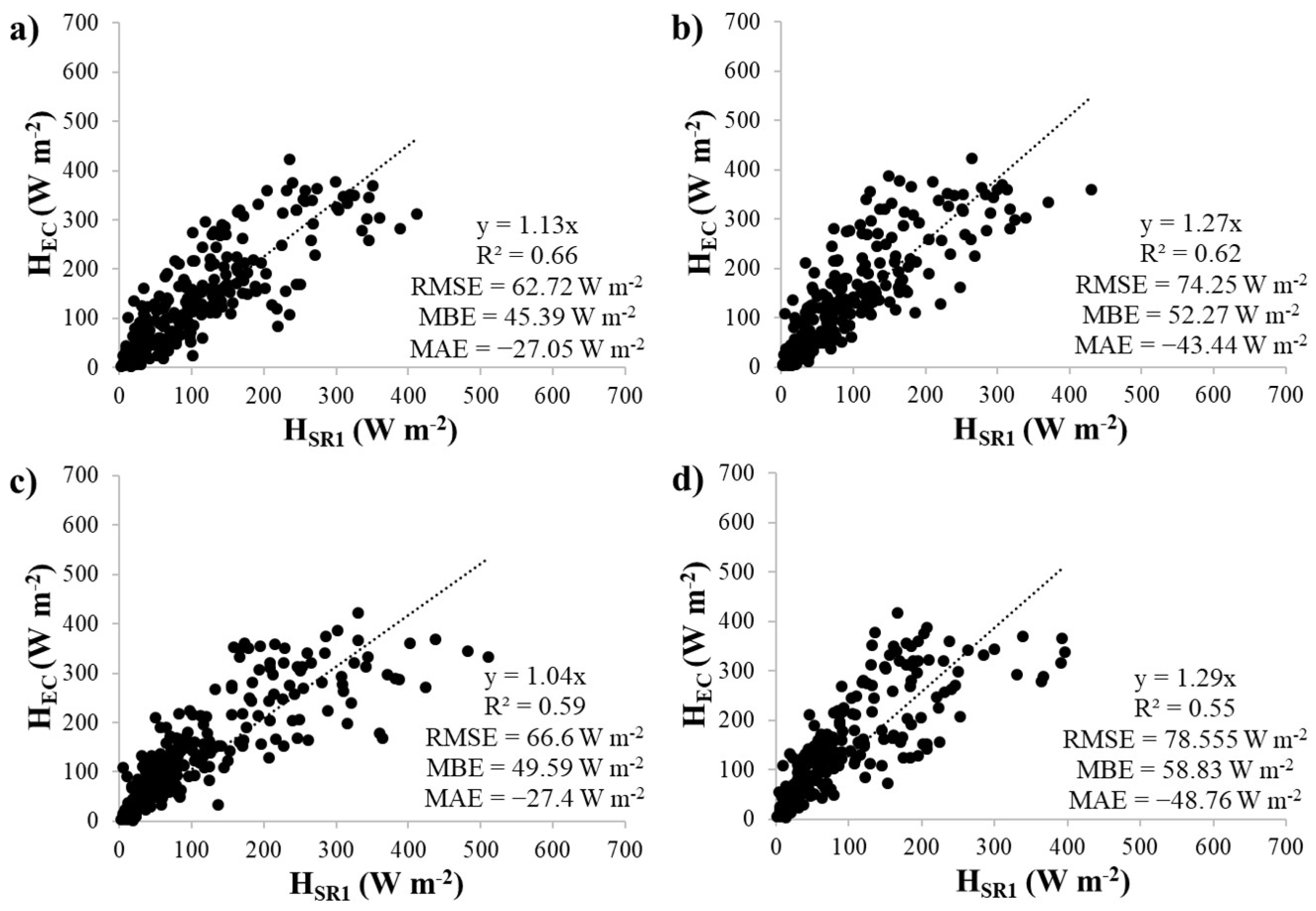
Linear regressions between half-hourly, uncalibrated HSR1 estimates and HEC measurements at the control and cut plots are shown in Figure 3 and Figure 4. Individual regressions were performed for each thermocouple and time lag combination. The α factors represented by the slope of the regressions ranged between 0.96 and 1.05 at the control plot and 1.04 and 1.29 at the cut plot. Similar α factors were found for the two measurement heights, however, higher α factors were obtained for the 0.8 s time lags than for the 0.4 s time lags.
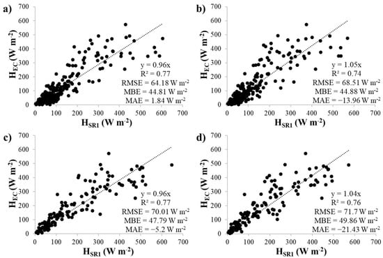
Figure 3.
Linear regression analysis between HSR1 and HEC at the control plot for the upper thermocouple using time lags of (a) 0.4 s and (b) 0.8 s and the lower thermocouple using time lags of (c) 0.4 s and (d) 0.8 s.

Figure 4.
Linear regression analysis between HSR1 and HEC at the cut plot for the upper thermocouple using time lags of (a) 0.4 s and (b) 0.8 s and the lower thermocouple using time lags of (c) 0.4 s and (d) 0.8 s.
The calibration regressions clearly showed that the optimal height and time lag for SR1 sampling at the site was the upper thermocouple and the 0.4 s time lag. Higher R2 values, lower RMSE and MBE values and MAE values closer to zero were obtained at both plots. Therefore, the HSR1 estimates were adjusted using these calculated α factors (0.96 and 1.13 for the control and cut plot, respectively), to obtain calibrated HSR1′ estimates.
3.3. Validity of SR1 and SRDT
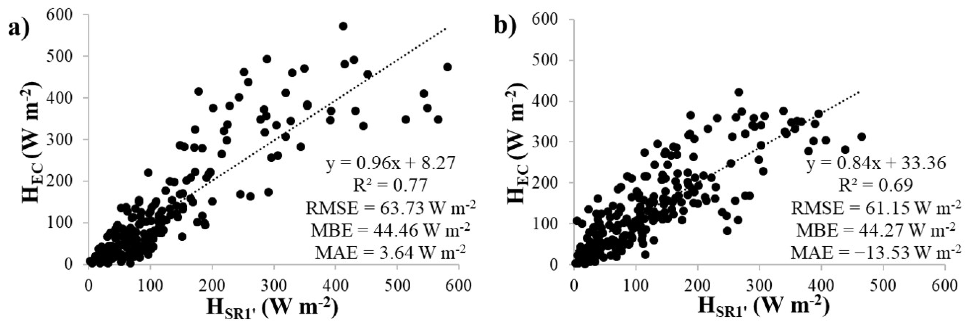
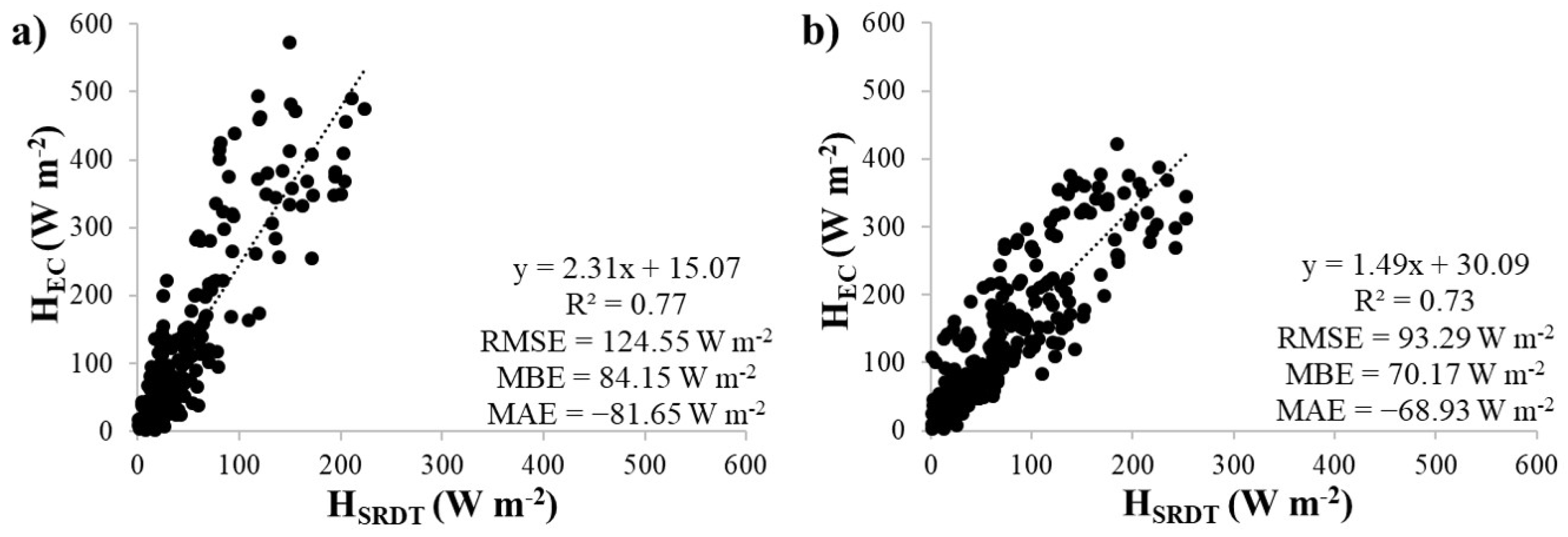
Linear regressions of the HSR1′ and HSRDT estimates were compared to the HEC measurements for the upper thermocouple and 0.4 s time lag at both plots (Figure 5 and Figure 6). The HSR1′ estimates agreed well with HEC, with slopes close to 1 (0.96 and 0.84 for the control and cut plots, respectively). However, the HSRDT estimates did not show good agreement with HEC, with slopes that well exceeded 1 (2.31 and 1.49 for the control and cut plots, respectively), indicating that HSRDT underestimated HEC. In addition, the SRDT approach predicted HEC with much higher errors (RMSE values of 124.55 W m−2 and 93.29 W m−2, MBE values of 84.15 W m−2 and 70.17 W m−2, and MAE values of −81.65 W m−2 and −68.93 W m−2 for the control and cut plots, respectively), compared to the errors predicted by the SR1 approach (RMSE values of 63.73 W m−2 and 61.15 W m−2, MBE values of 44.46 W m−2 and 44.27 W m−2, and MAE values of 3.64 W m−2 and −13.53 W m−2 for the control and cut plots, respectively).
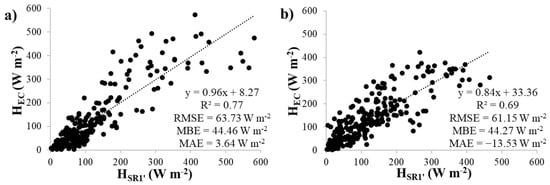
Figure 5.
Linear regression analysis between HSR1′ and HEC for the upper thermocouple using the 0.4 s time lag at the (a) control and (b) cut plots.
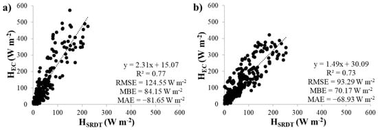
Figure 6.
Linear regression analysis between HSRDT and HEC for the upper thermocouple using the 0.4 s time lag at the (a) control and (b) cut plots.
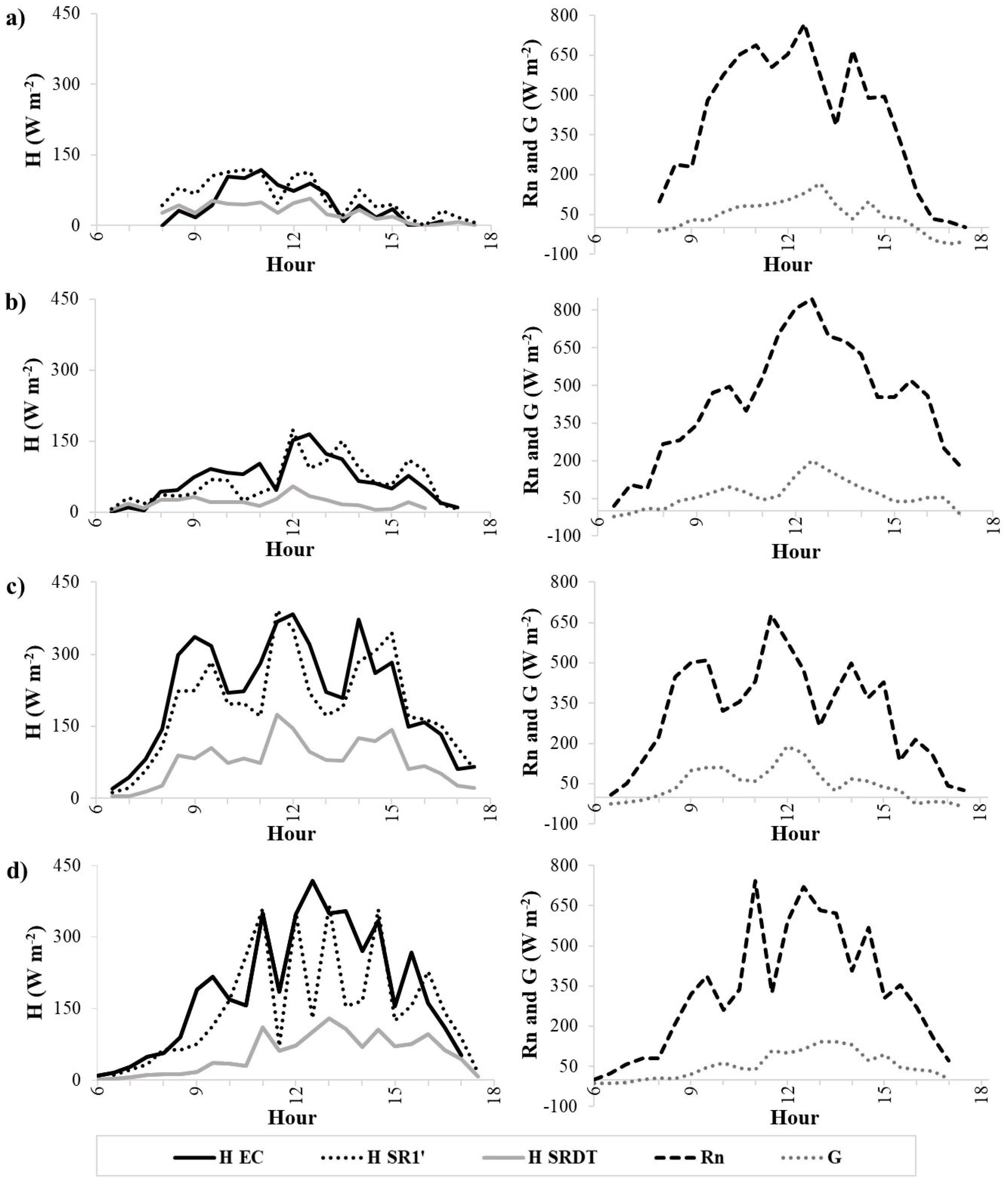
The diurnal variation of half-hourly HSR1′ and HSRDT for the upper thermocouple and 0.4 s time lag was compared against HEC for one day during the two campaigns at the plots (Figure 7), to further validate HSR1′ and HSRDT estimates against HEC measurements. The Rn and G measurements are also shown to better understand their relationship with HEC and HSR. The days shown were selected as those that were warm, sunny and had no rainfall. H for all methods was generally positive throughout the day, with the lowest values in the morning and late afternoon and the highest values around midday. HSR1 tended to agree well with HEC, however, it slightly underestimated HEC throughout the day of the spring campaign at the cut plot. HSRDT also tended to follow the HEC trends, but largely underestimated HEC. H for all methods followed the same diurnal trends as Rn and G. HEC, HSR1, HSRDT and Rn values were close to 0 in the early morning, increasing steadily until they peaked around noon. They then dropped back to around 0 in the early evening. G also peaked around noon, but was often negative in the morning and in the early evening hours.

Figure 7.
Diurnal variation of half-hourly HEC, HSR1′, HSRDT, Rn and G for one day during the summer campaign at the (a) control and (b) cut plot and the spring campaign at the (c) control and (d) cut plot.
Based on these statistics and observations, SR1 was deemed the most suitable SR approach for H estimation at the site. Therefore, HSR1′ estimates were used to estimate LE and ET for the long-term measurement period.
3.4. Long-Term Daily ET and Energy Balance Flux Measurements
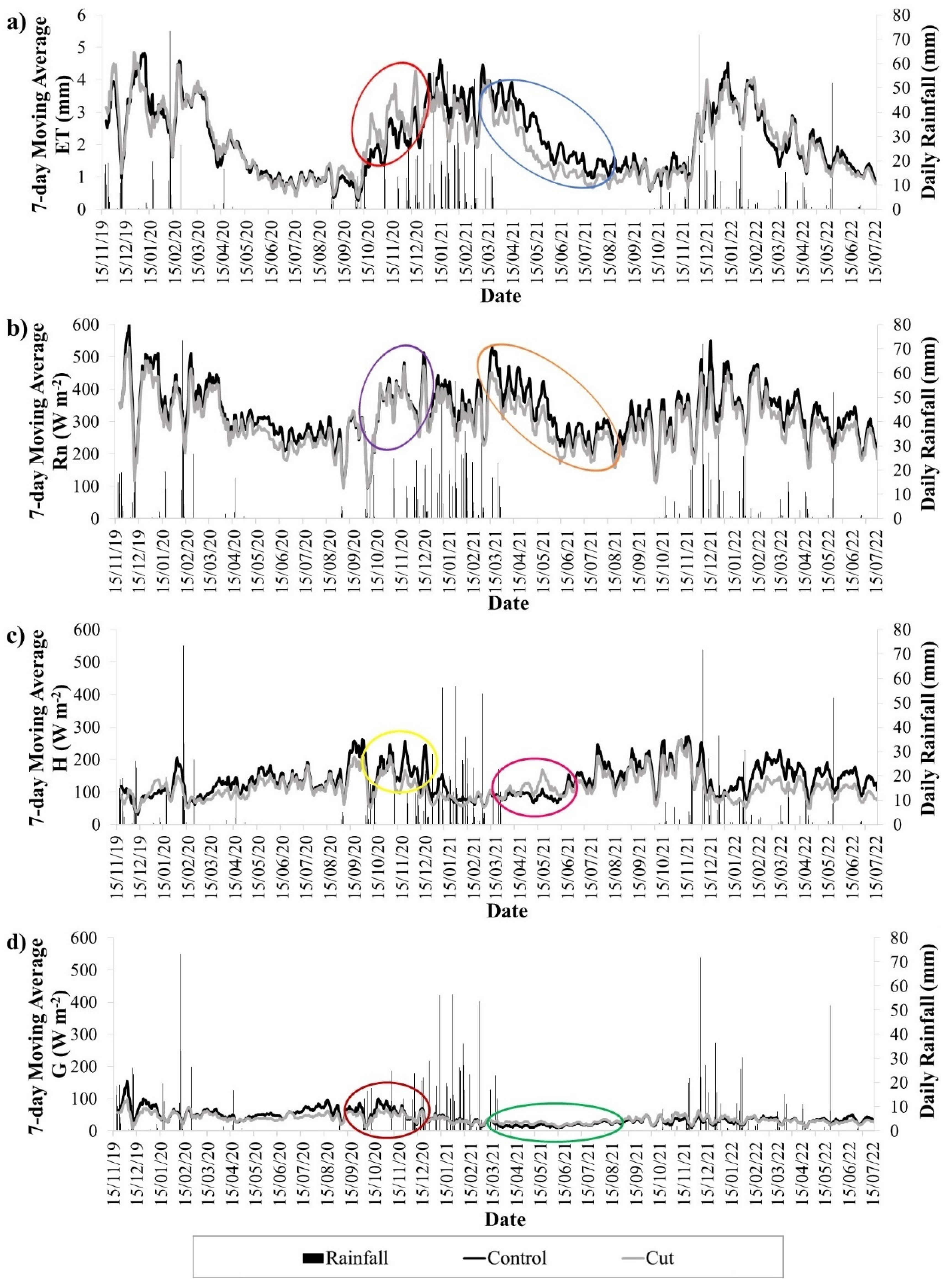
A 7-day moving average was calculated for the daily ET in an effort to minimize fluctuations and make trends more visible (Figure 8a). This revealed a strong seasonal pattern in ET at both plots, with high responses to rainfall. Higher ET occurred in the wetter summer months (December, January and February), averaging approximately 3 mm per day and reaching a maximum of approximately 5 mm per day, whereas the ET was much lower during the drier winter months (June, July and August), averaging approximately 1 mm per day. The lower ET in winter reflects the deciduous nature of the vegetation, resulting in a cessation of transpiration and ET primarily comprised of soil water evaporation by the end of the dry season.
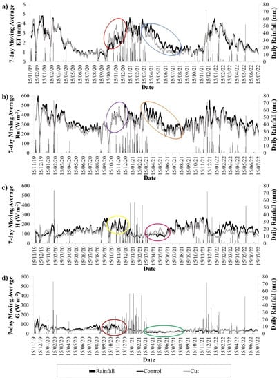
Figure 8.
7-Day moving averages for (a) ET, (b) Rn, (c) H and (d) G during unstable conditions at the control and cut plots, and the daily rainfall for the measurement period.
The control and cut plots had similar daily ET rates over most of the measurement period. However, after the first spring rains, the cut plot had higher ET peaks than the control plot, particularly for the 2020–2021 hydrological year (highlighted by the red oval, Figure 8a). This suggests that the grasses at the cut plot were able to expand their leaf area and initiate transpiration more rapidly than the mopane once soil water became available, which fits with phenology observations (pers. obs.). Mopane typically flushed their leaves after the grasses, and thereafter ET rates at the control plot rapidly increased until they equaled that of the cut plot for the remainder of the summer. As rainfall decreased in autumn, vegetation senesced, resulting in a rapid drop in the ET to low rates that continued throughout winter. Grass leaves generally senesced before mopane leaves, which was particularly evident in the autumn and winter of the 2020–2021 hydrological year when the control plot maintained higher ET rates than the cut plot (blue oval, Figure 8a). This slow decrease in ET and higher ET into autumn and winter of the mopane, in comparison to the grassland, shows how different vegetation structures and physiologies respond differently to the same climatic conditions. The offset in their responses may have been a result of the mopane keeping its leaves until late into the dry season to meet a seasonal growth cycle, or the mopane’s large rooting systems may have been able to access deeper soil water than the grasses as the upper soil layers dried up.
Figure 8b–d shows the 7-day moving averages of Rn, H and G at the control and cut plots over the measurement period. Rn followed similar diurnal trends and seasonal patterns as ET. H and G were smaller components of the energy balance and they did not replicate the ET trends well, nor was their seasonal pattern as strong as ET. Throughout the measurement period, the Rn was higher at the control plot than at the cut plot, indicating that the mopane trees resulted in less emitted and reflected infrared radiation, likely a result of their dense canopies. Therefore, more energy was available to drive ET at the control plot. However, during spring of the 2020–2021 hydrological year, there was a gradual increase in Rn at the cut plot, causing the difference in Rn between the plots to become smaller (purple oval, Figure 8b). Over this same period, H was lower at the cut plot than at the control plot (yellow oval, Figure 8c). These trends in Rn and H indicate that once soil water became available with the first spring rains, rapid greening of the grass swards occurred at the cut plot before the emergence of new leaves on the mopane at the control plot. The G was also higher at the control plot over this period (maroon oval, Figure 8d), indicating more shading of the soil layer and confirming that the grasses at the cut plot had a higher green leaf area. Therefore, there was higher potential for transpiration at the cut plot over this period. Over the autumn-winter period of the same 2020–2021 hydrological year, the difference in canopy cover is noticeable by the higher Rn at the control plot, indicating that the mopane still had active leaves, whereas the grassland was in senescence (orange oval, Figure 8b). H increased at the cut plot over this period (pink oval, Figure 8c), likely due to a lack of water available to the grasses, limiting their transpiration. Notably, the difference in G between the plots was minimal over this period (green oval, Figure 8d), indicating that the leaf area at both sites was similar, the difference being that the control likely had actively transpiring leaves with a high radiant absorptivity, whereas the grass in senescence had a higher reflectance.
3.5. Annual ET
The cumulative ET at the plots and the rainfall for the 2019–2020, 2020–2021 and 2021–2022 hydrological years of the study are shown in Figure 9a–c. The cumulative ET was comparable at the plots for the 2019–2020 and 2021–2022 years, totaling approximately 655 mm and 580 mm in 2019–2020 and 2021–2022, respectively. However, these years had missing ET data: for the first month and a half of 2019–2020 and the last two and a half months of 2021–2022. For the 2020–2021 year, for which there was a full data record, ET differences occurred between the plots. Increases in ET at the control plot lagged the cut plot, again indicating the more rapid growth and expansion of the grass leaf canopies following the first spring rainfall. Further into the growing season after the good summer rains, ET of the mopane increased rapidly, shown by the steeper slope of the accumulated ET at the control plot. The ET at the control plot eventually equaled the ET at the cut plot in the beginning of the dry season, and thereafter exceeded the ET at the cut plot for the duration of the dry season. In total, the annual ET at the control plot (854 mm) exceeded the annual ET at the cut plot (762 mm) by 12%.
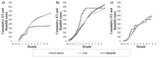
Figure 9.
The cumulative ET at the control and cut plots and rainfall for the (a) 2019–2020, (b) 2020–2021 and (c) 2021–2022 hydrological years.
The three hydrological years showed high inter-annual variability in the timing and amount of rainfall. 2019–2020 was the driest year and received an annual total rainfall of 364.7 mm, which was lower than the average for the site. However, this was significantly lower than the annual ET estimated for both plots. In fact, the annual ET exceeded the annual rainfall at the control and cut plots by 80%. 2020–2021 was a very wet year, receiving an annual rainfall of 770.9 mm, while the 2021–2022 year had a more typical rainfall of 511.6 mm (the latter is likely close to the total rainfall that occurred for the 2021–2022 year as the missing data fell over the dry season). For 2020–2021, the annual ET at the cut plot was similar to the annual rainfall, but the ET at the control plot exceeded the annual rainfall by 11%. For 2021–2022, the annual ET exceeded the annual rainfall at the control and cut plots by 15% and 13%, respectively.
The exceedance of the annual rainfall by the annual ET suggests that rainfall may not be the only source of water used by the vegetation during dry periods. Grasses have shallow roots and mopane are typically shallow-rooted trees, with most of their roots being found within the first 0.6 m of soil [58], therefore, it is probable that the vegetation supplemented its water use with water that accumulated in the soil during previous wet seasons. There is also the possibility that the vegetation, particularly the larger trees, used water from deeper soil stores or groundwater that rose to within the rooting depth by capillary action or hydraulic lift. The water tables are likely shallow, or perched, since the plots are located near the riparian area of the Klein Letaba River.
4. Discussion
4.1. SR1 Calibration
There are no previously determined α factors for semi-arid, savanna-type vegetation against which our α factors can be compared. However, previous studies that have carried out calibrations between HSR1 estimates and HEC measurements during unstable conditions for various plant canopies have reported α factors within the range of our estimates (our α factors ranged between 0.96 and 1.29). For example, in a montane catchment in South Africa, regression slopes of 0.89–0.92 have been reported for Leucosidea sericea and 0.81–0.86 for Pteridium aquilinium [21,31]. Internationally, regression slopes of 1.1 have been reported for rice in Spain [59], 0.97–1 for grass in the United States [60], 1.01–1.07 for cotton in Israel [23], 0.73 and 1.15 for rice and wheat crops in Egypt [61] and 0.68 for a tea plantation in China [62].
Similar α factors were found for the two measurement heights, despite previous studies having found that the α factor decreases with increasing measurement height [19,23,28,33,34,52,63,64]. However, higher α factors were obtained for the 0.8 s time lags than for the 0.4 s time lags, in agreement with Zapata and Martínez-Cob [63], Mengistu and Savage [28] and Gray et al. [21], who found higher α factors for longer time lags. Overall, HSR1 for the upper thermocouple and 0.4 s time lag showed best agreement against HEC.
4.2. Comparison between SR1, SRDT and EC for H Estimation
HSR1′ provided stronger regressions against HEC than HSRDT, with regression slopes closer to 1, lower RMSE and MBE values and MAE values closer to zero. The previous studies that compared HSRDT estimates and HEC measurements found better agreement than this study, which reported regression slopes of 2.31 and 1.49 for the control and cut plots, respectively. Gray et al. [21] and Gray et al. [31] reported regression slopes of 0.85–0.92 over Leucosidea sericea and 0.91–1.03 over Pteridium aquilinium, and Castellví and Snyder [39] reported a slope of 1.09 over grass in the United States. In addition, HSR1′ followed the diurnal trends more closely than HSRDT, which largely underestimated HEC. An adjustment to the correction factor would be required to use the SRDT approach at the site. However, the RMSE values for the HSR1′ regressions were relatively high in comparison to previous studies. The RMSE values for the HSR1′ regressions at the control and cut plots were 63.73 W m−2 and 78.55 W m−2, respectively, whereas Gray et al. [21] and Gray et al. [31], using the same instrumentation, reported RMSE’s of 36.74 W m−2–38.39 W m−2 over Leucosidea sericea and 39.56 W m−2–41.84 W m−2 over Pteridium aquilinium. Other international SR1 studies reported RMSE values ranging between 16 W m−2 and 42 W m−2 [33,59,60,62]. The RMSE values for the HSRDT regressions were also very high in comparison to other studies, with values of 124.55 W m−2 and 93.29 W m−2 for the control and cut plots, respectively. Gray et al. [21] and Gray et al. [31] reported RMSE’s of 36.18 W m−2–37.26 W m−2 over Leucosidea sericea and 38.77 W m−2–41.8 W m−2 over Pteridium aquilinium, and Castellví and Snyder [36] reported a RMSE of 52 W m−2 over grass. However, Castellví and Gavilán [20] compared LESRDT to lysimeter LE measurements over short fescue grass in Spain and found high RMSE’s, ranging between 93 W m−2 and 136 W m−2.
4.3. ET Measurements
A review of the available literature revealed only one study involving annual ET in situ measurements for a semi-arid savanna in South Africa. Dzikiti et al. [65] used data from a FluxNet EC system located in Skukuza in the Kruger National Park at an ecotone between Combretum apiculatum and Senegalia nigrescens savanna types. The EC flux tower is situated approximately 170 km south of the MGR, but has a higher MAP of approximately 547 mm. Over their two-year study period (2010 and 2011), Dzikiti et al. [65] measured an average annual ET of 610 mm and an average annual rainfall of only 323 mm. These results are within a fair range of our estimates for 2019–2020, the driest of the three years when the annual ET at both plots was significantly higher than the annual rainfall. Dzikiti et al. [65] also measured a maximum daily ET of 5 mm, which was the same as the maximum 7-day moving average ET estimated for all three summers of our study.
The annual ET at both plots exceeded the annual rainfall, indicating that the vegetation may access deep soil water stores or groundwater. In a previous study at the MGR site, Wedel et al. [66] determined that mopane used deeper soil water than grasses using stable isotopes, but no groundwater samples were taken to verify whether groundwater was a source of water used by the vegetation. Several studies that have measured ET for other vegetation types in South Africa have also found that the annual ET exceeded the annual rainfall. Dzikiti et al. [67] found that the annual ET of an arid woodland invaded by Prosopis was approximately four times higher than the rainfall. Isotopic analysis results confirmed that the Prosopis used groundwater. Palmer et al. [68] found that the annual ET of indigenous Albany thicket exceeded the annual rainfall by 7% over three hydrological years. Palmer et al. [68] suggested that the Albany thicket was likely supported by groundwater, but this was not confirmed.
5. Conclusions
The SR1 approach with EC calibration was found to be a viable method for estimating ET in a mopane-encroached, semi-arid savanna located in north-eastern South Africa. Over the three hydrological years of the study, ET was highly seasonal and was typically highest during the wet season when it responded to increased soil water availability and increased Rn. For the two drier years of the study, the removal of mopane trees had little effect on ET and all rainfall was evaporated irrespective of the density of woody plants. However, for the wettest year of the study, the annual ET at the control plot (mopane) was 12% higher than at the cut plot (grassland). These results support the hypothesis that WE in semi-arid savannas can increase ET, at least during years of above-average rainfall, and thus may reduce groundwater and soil water profile recharge. Another significant finding of the study was that the annual ET at both plots was able to exceed the annual rainfall. Further isotope studies are needed to confirm the water sources used by the vegetation, and to understand the source of the accumulated water that is available in dry years. Further research on ET-soil water processes at the MGR is also recommended, to advance our understanding of the relationship between vegetation structure, vegetation water consumption and water supplies in semi-arid savannas.
Author Contributions
Conceptualization, T.A.A., M.L.W.T. and A.D.C.; methodology, T.A.A., M.L.W.T., A.D.C. and A.M.S.; software, T.A.A., M.L.W.T. and A.D.C.; validation, T.A.A., M.L.W.T. and A.D.C.; formal analysis, T.A.A.; investigation, T.A.A., M.L.W.T. and A.M.S.; resources, T.A.A., M.L.W.T., A.D.C. and A.M.S.; data curation, T.A.A., M.L.W.T. and A.D.C.; writing—original draft preparation, T.A.A.; writing—review and editing, M.L.W.T., A.D.C. and A.M.S.; visualization, T.A.A.; supervision, M.L.W.T. and A.D.C.; project administration, M.L.W.T. and A.M.S.; funding acquisition, M.L.W.T. All authors have read and agreed to the published version of the manuscript.
Funding
This research was funded by the South African Environmental Observation Network (SAEON) business unit of the National Research Foundation (NRF) (ESS grant 118601).
Data Availability Statement
Data available on request.
Acknowledgments
The authors acknowledge the South African Environmental Observation Network (SAEON) business unit of the National Research Foundation (NRF) for administrative and technical support. Rion Lerm, Peace Nkuna and Byron Gray for their assistance with the set-up and maintenance of instrumentation and for data collection. Finally, the Mthimkhulu Tribal Authority for permitting the research at the site.
Conflicts of Interest
The authors declare no conflict of interest.
References
- Sala, O.E.; Maestre, F.T. Grass–woodland transitions: Determinants and consequences for ecosystem functioning and provisioning of services. J. Ecol. 2014, 102, 1357–1362. [Google Scholar] [CrossRef]
- Deng, Y.; Li, X.; Shi, F.; Hu, X. Woody plant encroachment enhanced global vegetation greening and ecosystem water-use efficiency. Glob. Ecol. Biogeogr. 2021, 30, 2337–2353. [Google Scholar] [CrossRef]
- Archer, S.R.; Andersen, E.M.; Predick, K.I.; Schwinning, S.; Steidl, R.J.; Woods, S.R. Woody Plant Encroachment: Causes and Consequences. In Rangeland Systems: Processes, Management and Challenges; Briske, D.D., Ed.; Springer: Gewerbestrasse, Switzerland, 2017; pp. 25–84. [Google Scholar]
- Stafford, W.; Birch, C.; Etter, H.; Blanchard, R.; Mudavanhu, S.; Angelstame, P.; Blignaut, J.; Ferreira, L.; Marais, C. The economics of landscape restoration: Benefits of controlling bush encroachment and invasive plant species in South Africa and Namibia. Ecosys. Serv. 2017, 27, 193–202. [Google Scholar] [CrossRef]
- Kambatuku, J.R.; Cramer, M.D.; Ward, D. Overlap in soil water sources of savanna woody seedlings and grasses. Ecohydrology 2013, 6, 464–473. [Google Scholar] [CrossRef]
- Huxman, T.E.; Wilcox, B.P.; Breshears, D.D.; Scott, R.L.; Snyder, K.A.; Small, E.E.; Hultine, K.; Pockman, W.T.; Jackson, R.B. Ecohydrological implications of woody plant encroachment. Ecology 2005, 86, 308–319. [Google Scholar] [CrossRef]
- Acharya, B.S.; Hao, Y.; Ochsner, T.E.; Zou, C.B. Woody plant encroachment alters soil hydrological properties and reduces downward flux of water in tallgrass prairie. Plant Soil 2017, 414, 379–391. [Google Scholar] [CrossRef]
- Stevens, N. What shapes the range edge of a dominant African savanna tree, Colophospermum mopane? A demographic approach. Ecol. Evol. 2021, 11, 3726–3736. [Google Scholar] [CrossRef]
- MacGregor, S.D.; O’Connor, T.G. Patch dieback of Colophospermum mopane in a dysfunctional semi-arid African savanna. Austral Ecol. 2002, 27, 385–395. [Google Scholar] [CrossRef]
- Whitecross, M.A.; Archibald, S.; Witkowski, E.T.F. Do freeze events create a demographic bottleneck for Colophospermum mopane? S. Afr. J. Bot. 2012, 83, 9–18. [Google Scholar] [CrossRef]
- Makhado, R.A.; Mapaure, I.; Potgieter, M.J.; Luus-Powell, W.J.; Saidi, A.T. Factors influencing the adaptation and distribution of Colophospermum mopane in southern Africa’s mopane savannas—A review. Bothalia 2014, 44, 1–9. [Google Scholar] [CrossRef]
- Smit, G.N. An approach to tree thinning to structure southern African savannas for long-term restoration from bush encroachment. J. Environ. Manag. 2004, 71, 179–191. [Google Scholar] [CrossRef] [PubMed]
- Smit, G.N.; Rethman, N.F.G. The influence of tree thinning on the soil water in a semi-arid savanna of southern Africa. J. Arid Environ. 2000, 44, 41–59. [Google Scholar] [CrossRef]
- Schreiner-McGraw, A.P.; Vivoni, E.R.; Ajami, H.; Sala, O.E.; Throop, H.L.; Peters, D.P.C. Woody Plant Encroachment has a Larger Impact than Climate Change on Dryland Water Budgets. Sci. Rep. 2020, 10, 8112. [Google Scholar] [CrossRef] [PubMed]
- Afinowicz, J.D.; Munster, C.L.; Wilcox, B.P. Modelling effects of brush management on the rangeland water budget: Edwards Plateau, Texas. J. Am. Water Resour. Assoc. 2005, 41, 181–193. [Google Scholar] [CrossRef]
- Scott, R.L.; Huxman, T.E.; Williams, D.G.; Goodrich, D.C. Ecohydrological impacts of woody-plant encroachment: Seasonal patterns of water and carbon dioxide exchange within a semiarid riparian environment. Glob. Chang. Biol. 2006, 12, 311–324. [Google Scholar] [CrossRef]
- Kormos, P.R.; Marks, D.; Pierson, F.B.; Williams, C.J.; Hardegree, S.P.; Havens, S.; Hedrick, A.; Bates, J.D.; Svejcar, T.J. Ecosystem water availability in Juniper versus Sagebrush snow-dominated rangelands. Rangel. Ecol. Manag. 2017, 70, 116–128. [Google Scholar] [CrossRef]
- Hu, Y.; Buttar, N.A.; Tanny, J.; Snyder, R.L.; Savage, M.J.; Lakhiar, I.A. Surface renewal application for estimating evapotranspiration: A review. Adv. Meteorol. 2018, 2018, 1690714. [Google Scholar] [CrossRef]
- Poblete-Echeverría, C.; Sepúlveda-Reyes, D.; Ortega-Farías, S. Effect of height and time lag on the estimation of sensible heat flux over a drip-irrigated vineyard using the surface renewal (SR) method across distinct phenological stages. Agric. Water Manag. 2014, 141, 74–83. [Google Scholar] [CrossRef]
- Castellví, F.; Gavilán, P. Estimation of the latent heat flux over irrigated short fescue grass for different fetches. Atmosphere 2021, 12, 322. [Google Scholar] [CrossRef]
- Gray, B.A.; Toucher, M.L.; Savage, M.J.; Clulow, A.D. The potential of surface renewal for determining sensible heat flux for indigenous vegetation for a first-order montane catchment. Hydrol. Sci. J. 2021, 66, 1015–1027. [Google Scholar] [CrossRef]
- Pozníková, G.; Fischera, M.; van Kesterend, B.; Orsága, M.; Hlavinkaa, P.; Žalud, Z.; Trnka, M. Quantifying turbulent energy fluxes and evapotranspiration in agricultural field conditions: A comparison of micrometeorological methods. Agric. Water Manag. 2018, 209, 249–263. [Google Scholar] [CrossRef]
- Rosa, R.; Dicken, U.; Tanny, J. Estimating evapotranspiration from processing tomato using the surface renewal technique. Biosyst. Eng. 2013, 114, 406–413. [Google Scholar] [CrossRef]
- Zapata, N.; Martínez-Cob, A. Evaluation of the surface renewal method to estimate wheat evapotranspiration. Agric. Water Manag. 2002, 55, 141–157. [Google Scholar] [CrossRef]
- Suvočarev, K.; Shapland, T.M.; Snyder, R.L.; Martinez-Cob, A. Surface renewal performance to independently estimate sensible and latent heat fluxes in heterogeneous crop surfaces. J. Hydrol. 2014, 509, 83–93. [Google Scholar] [CrossRef]
- Haymann, N.; Lukyanova, V.; Tanny, J. Effects of variable fetch and footprint on surface renewal measurements of sensible and latent heat fluxes in cotton. Agric. For. Meteorol. 2019, 268, 63–73. [Google Scholar] [CrossRef]
- Savage, M.J. Estimation of grass reference evaporation and sensible heat flux using surface renewal and Monin-Obukhov similarity theory: A simple implementation of an iterative method. J. Hydrol. 2017, 547, 742–754. [Google Scholar] [CrossRef]
- Mengistu, M.G.; Savage, M.J. Open water evaporation estimation for a small shallow reservoir in winter using surface renewal. J. Hydrol. 2010, 380, 27–35. [Google Scholar] [CrossRef]
- Clulow, A.D.; Everson, C.S.; Mengistu, M.G.; Jarmain, C.; Jewitt, G.P.W.; Price, J.S.; Grundling, P.L. Measurement and modelling of evaporation from a coastal wetland in Maputaland. Hydrol. Earth Syst. Sci. 2012, 16, 3233–3247. [Google Scholar] [CrossRef]
- Dye, P.J.; Gush, M.B.; Everson, C.S.; Jarmain, C.; Clulow, A.; Mengistu, M.; Geldenhuys, C.J.; Wise, R.; Scholes, R.J.; Archibald, S.; et al. Water-Use in Relation to Biomass of Indigenous Tree Species in Woodland, Forest and/or Plantation Conditions; Report TT361/08; Water Research Commission: Pretoria, South Africa, 2008. [Google Scholar]
- Gray, B.A.; Toucher, M.L.; Savage, M.J.; Clulow, A.D. Seasonal evapotranspiration over an invader vegetation (Pteridium aquilinum) in a degraded montane grassland using surface renewal. J. Hydrol. Reg. 2022, 40, 101012. [Google Scholar] [CrossRef]
- Paw U, K.T.; Qiu, J.; Su, H.B.; Watanabe, T.; Brunet, Y. Surface renewal analysis: A new method to obtain scalar fluxes. Agric. For. Meteorol. 1995, 74, 119–137. [Google Scholar] [CrossRef]
- Rosa, R.; Tanny, J. Surface renewal and eddy covariance measurements of sensible and latent heat fluxes of cotton during two growing seasons. Biosyst. Eng. 2015, 136, 149–161. [Google Scholar] [CrossRef]
- Castellví, F. Combining surface renewal analysis and similarity theory: A new approach for estimating sensible heat flux. Water Resour. Res. 2004, 40, W05201. [Google Scholar] [CrossRef]
- Mengistu, M.G.; Savage, M.J. Surface renewal method for estimating sensible heat flux. Water SA 2010, 36, 9–18. [Google Scholar] [CrossRef]
- Castellví, F.; Snyder, R.L. On the performance of surface renewal analysis to estimate sensible heat flux over two growing rice fields under the influence of regional advection. J. Hydrol. 2009, 375, 546–553. [Google Scholar] [CrossRef]
- Snyder, R.L.; Spano, D.; Paw U, K.T. Surface renewal analysis for sensible and latent heat flux density. Bound.-Layer Meteorol. 1996, 77, 249–266. [Google Scholar] [CrossRef]
- Castellví, F.; Perez, P.J.; Ibañez, M. A method based on high frequency temperature measurements to estimate sensible heat flux avoiding the height dependence. Water Resour. Res. 2002, 38, 1084. [Google Scholar] [CrossRef]
- Castellví, F.; Snyder, R.L. Combining the dissipation method and surface renewal analysis to estimate scalar fluxes from the time traces over rangeland grass near Ione (California). Hydrol. Process. 2009, 23, 842–857. [Google Scholar] [CrossRef]
- Hsieh, C.I.; Katul, G.G. Dissipation methods, Taylor’s hypothesis, and stability correction functions in the atmospheric surface layer. J. Geophys. Res. 1997, 102, 16391–16405. [Google Scholar] [CrossRef]
- Ferreria, S.; Harmse, A. Kruger National Park: Tourism development and issues around the management of large numbers of tourists. J. Ecotourism 2014, 13, 16–34. [Google Scholar] [CrossRef]
- Acocks, J.P.H. Veld Types of South Africa, 3rd ed.; Memoirs of the Botanical Survey of South Africa No. 57; Botanical Research Institute: Pretoria, South Africa, 1988. [Google Scholar]
- Mucina, L.; Rutherford, M.C. The Vegetation of South Africa, Lesotho and Swaziland; Strelitzia 19, South African National Biodiversity Institute: Pretoria, South Africa, 2006. [Google Scholar]
- Kennedy, A.D.; Potgieter, A.L.F. Fire season affects size and architecture of Colophospermum mopane in southern African savannas. Plant Ecol. 2003, 167, 179–192. [Google Scholar] [CrossRef]
- Stevens, N.; Swemmer, A.M.; Ezzy, L.; Erasmus, B.F.N. Investigating potential determinants of the distribution limits of a savanna woody plant: Colophospermum mopane. J. Veg. Sci. 2013, 25, 363–373. [Google Scholar] [CrossRef]
- Soil Classification Working Group. Soil Classification: A Natural and Anthropogenic System for South Africa; Agricultural Research Council—Institute for Soil, Climate and Water: Pretoria, South Africa, 2018. [Google Scholar]
- Burba, G. Eddy Covariance Method for Scientific, Industrial, Agricultural and Regulatory Applications; LI-COR Biosciences: Lincoln, NE, USA, 2013. [Google Scholar]
- Campbell Scientific. EASYFLUX DL CR3000OP for CR3000 and Open-Path Eddy-Covariance System Revision: 3/18. 2020. Available online: https://s.campbellsci.com/documents/us/manuals/easyflux-dl.pdf (accessed on 14 August 2022).
- Van Atta, C.W. Effect of coherent structures on structure functions of temperature in the atmospheric boundary layer. Arc. Mech. 1977, 29, 161–171. [Google Scholar]
- Campbell Scientific. Model HFP01SC Self-Calibrating Soil Heat Flux Plate Revision: 10/16. 2016. Available online: https://s.campbellsci.com/documents/us/manuals/hfp01sc.pdf (accessed on 14 August 2022).
- Shapland, T.M.; McElrone, A.J.; Snyder, R.L.; Paw U, K.T. Structure function analysis of two-scale scalar ramps. Part II: Ramp characteristics and surface renewal flux estimation. Bound.-Layer Meteorol. 2012, 145, 27–44. [Google Scholar] [CrossRef]
- Spano, D.; Snyder, R.L.; Duce, P.; Paw U, K.T. Estimating sensible and latent heat flux densities from grapevine canopies using surface renewal. Agric. For. Meteorol. 2000, 104, 171–183. [Google Scholar] [CrossRef]
- Castellví, F.; Snyder, R.L. A comparison between latent heat fluxes over grass using a weighing lysimeter and surface renewal analysis. J. Hydrol. 2010, 381, 213–220. [Google Scholar] [CrossRef]
- Rinne, J.; Ammann, C. Disjunct Eddy Covariance Method. In Eddy Covariance A Practical Guide to Measurement and Data Analysis; Aubinet, M., Vesala, T., Papale, D., Eds.; Springer: Dordrecht, The Netherlands, 2012; pp. 291–307. [Google Scholar]
- Foken, T.; Leuning, R.; Oncley, S.R.; Mauder, M.; Aubinet, M. Corrections and data quality control. In Eddy Covariance; Aubinet, M., Vesala, T., Papale, D., Eds.; Springer: Dordrecht, The Netherlands, 2012; pp. 85–131. [Google Scholar]
- Savage, M.J. Web-Based Teaching, Learning and Research Using Real-Time Data from Field-Based Agrometeorological Measurement Systems. MScAgric Dissertation, University of KwaZulu-Natal, Durban, South Africa, 2014. [Google Scholar]
- Dimitriadou, S.; Nikolakopoulos, K.G. Development of the Statistical Errors Raster Toolbox with Six Automated Models for Raster Analysis in GIS Environments. Remote Sens. 2022, 14, 5446. [Google Scholar] [CrossRef]
- Smit, G.N.; Rethman, N.F.G. Root biomass, depth distribution and relations with leaf biomass of Colophospermum mopane. S. Afr. J. Bot. 1998, 64, 38–43. [Google Scholar] [CrossRef]
- Castellví, F.; Martínez-Cob, A.; Pérez-Coveta, O. Estimating sensible and latent heat fluxes over rice using surface renewal. Agric. For. Meteorol. 2006, 139, 164–169. [Google Scholar] [CrossRef]
- Castellví, F.; Snyder, R.L.; Baldocchi, D.D. Surface energy-balance closure over rangeland grass using the eddy covariance method and surface renewal analysis. Agric. For. Meteorol. 2008, 148, 1147–1160. [Google Scholar] [CrossRef]
- El-Magd, A.A.; Attaher, S.M.; Snyder, R.L. Evaluation of surface renewal vs. eddy covariance methods to estimate cereal crops evapotranspiration. J. Soil Sci. Agric. Eng. 2020, 11, 845–851. [Google Scholar]
- Wang, J.; Buttar, N.A.; Hu, Y.; Lakhiar, I.A.; Javed, Q.; Shabbir, A. Estimation of sensible and latent heat fluxes using surface renewal method: Case study of a tea plantation. Agronomy 2021, 11, 179. [Google Scholar] [CrossRef]
- Zapata, N.; Martínez-Cob, A. Estimation of sensible and latent heat flux from natural sparse vegetation surfaces using surface renewal. J. Hydrol. 2001, 254, 215–228. [Google Scholar] [CrossRef]
- Mekhmandarov, Y.; Pirkner, M.; Achiman, O.; Tanny, J. Application of the surface renewal technique in two types of screenhouses: Sensible heat flux estimates and turbulence characteristics. Agric. For. Meteorol. 2015, 203, 229–242. [Google Scholar] [CrossRef]
- Dzikiti, S.; Jovanovic, N.Z.; Bugan, R.D.H.; Ramoelo, A.; Majozi, N.P.; Nickless, A.; Cho, M.A.; Le Maitre, D.C.; Ntshidi, Z.; Pienaar, H.H. Comparison of two remote sensing models for estimating evapotranspiration: Algorithm evaluation and application in seasonally arid ecosystems in South Africa. J. Arid Land 2019, 11, 495–512. [Google Scholar] [CrossRef]
- Wedel, E.R.; Nippert, J.B.; Swemmer, A.M. Lowveld savanna bush cutting alters tree-grass interactions. In Proceedings of the XXIV International Grassland Congress, Virtual, 25–29 October 2021. [Google Scholar]
- Dzikiti, S.; Ntshidi, Z.; Le Maitre, D.C.; Bugan, R.D.H.; Mazvimavi, D.; Schachtschneider, K.; Jovanovic, N.Z.; Pienaar, H.H. Assessing water use by Prosopis invasions and Vachellia karroo trees: Implications for groundwater recovery following alien plant removal in an arid catchment in South Africa. For. Ecol. Manag. 2017, 398, 153–163. [Google Scholar] [CrossRef]
- Palmer, A.R.; Ezenne, G.I.; Choruma, D.J.; Gwate, O.; Mantel, S.K.; Tanner, J.L. A comparison of three models used to determine water fluxes over the albany thicket, Eastern Cape, South Africa. Agric. For. Meteorol. 2020, 288–289, 107984. [Google Scholar] [CrossRef]
Disclaimer/Publisher’s Note: The statements, opinions and data contained in all publications are solely those of the individual author(s) and contributor(s) and not of MDPI and/or the editor(s). MDPI and/or the editor(s) disclaim responsibility for any injury to people or property resulting from any ideas, methods, instructions or products referred to in the content. |
© 2022 by the authors. Licensee MDPI, Basel, Switzerland. This article is an open access article distributed under the terms and conditions of the Creative Commons Attribution (CC BY) license (https://creativecommons.org/licenses/by/4.0/).


